Identification and Machine Learning Prediction of Nonlinear Behavior in a Robotic Arm System

Abstract

In this study, the subject of investigation was the dynamic double pendulum crank mechanism used in a robotic arm. The arm is driven by a DC motor though the crank system and connected to a fixed side with a mount that includes a single spring and damping. Robotic arms are now widely used in industry, and the requirements for accuracy are stringent. There are many factors that can cause the induction of nonlinear or asymmetric behavior and even excite chaotic motion. In this study, bifurcation diagrams were used to analyze the dynamic response, including stable symmetric orbits and periodic and chaotic motions of the system under different damping and stiffness parameters. Behavior under different parameters was analyzed and verified by phase portraits, the maximum Lyapunov exponent, and Poincaré mapping. Firstly, to distinguish instability in the system, phase portraits and Poincaré maps were used for the identification of individual images, and the maximum Lyapunov exponents were used for prediction. GoogLeNet and ResNet-50 were used for image identification, and the results were compared using a convolutional neural network (CNN). This widens the convolutional layer and expands pooling to reduce network training time and thickening of the image; this deepens the network and strengthens performance. Secondly, the maximum Lyapunov exponent was used as the key index for the indication of chaos. Gaussian process regression (GPR) and the back propagation neural network (BPNN) were used with different amounts of data to quickly predict the maximum Lyapunov exponent under different parameters. The main finding of this study was that chaotic behavior occurs in the robotic arm system and can be more efficiently identified by ResNet-50 than by GoogLeNet; this was especially true for Poincaré map diagnosis. The results of GPR and BPNN model training on the three types of data show that GPR had a smaller error value, and the GPR-21 × 21 model was similar to the BPNN-51 × 51 model in terms of error and determination coefficient, showing that GPR prediction was better than that of BPNN. The results of this study allow the formation of a highly accurate prediction and identification model system for nonlinear and chaotic motion in robotic arms.

1. Introduction

The rise in factory automation has resulted in large numbers of mechanical processes being carried out by automatic robotic arms instead of manpower. This increases the production rate and reduces cost, but there are still many shortcomings in robotic arm function and execution. Under specific operational conditions, a robotic arm system can suffer from irregular vibration, which can lead to chattering and uneven product quality. The damping coefficient, rigidity, speed of arm movement and angle, the mass of internal parts, and even arm length may all be factors that can induce nonlinear vibration. To solve this problem and improve the stability of the robotic arm system, Sigeru Futami et al. [1] installed accelerometers on three axes of a robotic arm and fed the signals to corresponding actuators through a phase compensation circuit. This eliminated the resonance and stabilized the arm. Jam et al. [2] proposed a shock absorbing system composed of a spring, a mass, and viscous damping, which effectively suppressed vibration. To gain a clear understanding of robotic arm instability, it is necessary to take nonlinear dynamic systems into consideration. Consequently, many recent in-depth studies of the problem have involved chaos theory analyses. Ambarish Goswami et al. [3] carried out nonlinear analysis of the dynamics of a biped robot, using ground slope, mass, and foot length as parameters. They showed that a series of cycle doubling behavior was involved in a simple robot walking model. Shrinivas Lankalapalli et al. [4,5] used PD controllers to regulate a dual rotary joint mechanism and analyzed the chaotic phenomena. The dynamic behavior after feedback was observed, and the results were verified by maximum Lyapunov exponents showing that chaotic behavior arose from extremely low proportional and differential gain. Sado and Gajos [6] studied a three-degrees-of-freedom suspension double pendulum mechanism, simulating the excited vibration generated by the flexible element between the fixed ends. The damping coefficient was used as the bifurcation parameter to analyze the chaos. In recent years, robot manipulators are often tasked with working in environments with vibrations and are subject to load uncertainty. Providing an accurate tracking control design with implementable torque input for these robots has become important. Tolgay et al. [7] presented a robust and adaptive control scheme based on a sliding mode control accompanied by proportional derivative control terms for the trajectory tracking of nonlinear robotic manipulators in the presence of system uncertainties and external disturbances. The Lyapunov theory was used to prove stability of the proposed method, and a four link SCARA robot was used to demonstrate efficacy of the proposed method via simulation. Razzaghi et al. [8] introduced a unique hopping robot based on the inertial actuation concept, which could navigate in three-dimensional environments. They also applied sliding mode control based on the Lyapunov approach, and a state-dependent Riccati equation-based optimal controller was also designed. Mustafa et al. [9] proposed joint space tracking control design in the presence of uncertain nonlinear torque caused by external vibration and payload variation. A Lyapunov-based method was utilized to guarantee the stability and control. Dachang et al. [10] developed an adaptive back-stepping sliding mode control to solve precise trajectory tracking in the presence of external disturbances in a complex environment. The dynamic response characteristics of a two-link robotic manipulator was analyzed using a back-stepping algorithm based on the Lyapunov theory to stabilize the sliding mode controller. All these studies showed that damping parameters have a considerable influence on the system, and may even produce nonlinear vibrations. However, few studies have been made on the stiffness parameters, which have a very important effect on the stability of the robotic arm. Therefore, the bifurcation dynamic characteristics of the vibration behavior caused by stiffness have been analyzed in this study.

The development of machine learning can be shallow or deep. The shallow part has three categories: supervised, unsupervised, and reinforcement learning [11]. The approach used in this study was supervised learning, which can be regressive or classificatory. Regression is related to continuous data training and numerical prediction results. Classification is used with discrete data to predict results from training and labeling. Shallow machine learning is widely used in prediction and diagnosis, and the algorithms have become very diverse. Therefore, many studies and much effort has been expended on the derivation of algorithms for different applications and on the reduction of time cost. Praveenkumar et al. [12] designed an accelerometer based on the concept of machine learning for the analysis of automobile gearboxes and used it to diagnose the various vibration signals from faulty gears. Mohandes et al. [13] made actual data prediction in the application of wind speed; they compared the support vector machine (SVM) with multi-layer perceptron (MLP) and showed that, in terms of root mean square error, SVM was superior to MLP. In material technology, wear resistance has become very important. Osman Altay et al. [14] predicted the wear of different ferroalloy coatings to save production cost and man-hours using linear regression (LR), support vector machine, and Gaussian process regression (GPR). The prediction results show that the success rate of SVM and GPR were similar, and LR showed the lowest power consumption. Guofeng Wang et al. [15] used Gaussian mixture regression (GMR) to predict continuous tool wear and combined it with multiple linear regression (MLR), radial basis function kernel (RBF), and a back propagation algorithm (BP). The results proved the relative superiority of GMR [16].

In many deep learning applications, the training model often suffers from an insufficiency of training data, and this has led to the development of transfer learning. This method uses the trained model to migrate to new models and accelerate their establishment. For example, in image recognition there is a certain correlation in the image training process, so a model that has been trained on a large number of images can be used to make up for a situation where there are too few images of the target. The existing models can be effectively used to deal with different scenes. In addition, transfer learning can avoid the need to start the training model from scratch. Some recent studies [17,18,19] based on transfer learning have used pre-trained CNN models, ResNet-50, and DenseNet-161 to classify pathological images. An accuracy of 98.87% was obtained by ResNet-50 using color images, and an accuracy of 97.89% by DenseNet-161 on gray images. Mohamed Marei et al. [20] carried out effective prediction and health management on CNC machining processes, used transfer learning to judge the wear of cutting tools comparing six classic CNN models. The results were similar to those produced by ResNet-18. The accuracy rate was as high as 84%, showing migration learning to be effective in this application.

Investigation of the efficacy of CNN and the prediction and identification of nonlinear motion in robotic arm systems in the past are relatively rare [21,22,23]. In this study, GoogLeNet and ResNet-50 were used for image identification in robotic arm system behavior and also to predict nonlinear motion and chaos. The maximum Lyapunov exponent was used for verification of chaos and for prediction under different system parameters using GPR and BPNN. The results may prove useful as a guideline for nonlinear behavior control and as a reference for enterprises in the prediction and prevention of nonlinear motion in robotic arms.

2. Theoretical Analysis

The Principles of Robotic Arm Operation

A schematic of the robotic arm system used in this study is shown in Figure 1. It is driven by a DC motor, and the vertical displacement of the motor is controlled by the bottom crank mechanism connecting by a spring. The motor is also connected to the upper fixed side by a spring and a damper for stability control [24]. The governing equations of this mechanical robotic arm are shown in (1)–(4).

A coupled air bearing system with five degrees of freedom in five directions, x, y, z, θ_x, and θ_y,, was designed. Comparisons of the performance of single thrust and radial bearings were also conducted. The purpose was to find the optimal design criteria for a coupled air bearing system and to get a full picture of their different motion behaviors. Based on the narrow groove theory, the non-dimensional Reynolds equations of this coupled air bearing system can be derived, which include lubrication equations of thrust and radial bearings, as shown in Equations (1) and (2):

$$\begin{array}{cc}\hfill \left(M+M_1+M_2\right)\ddot{x}& +c\dot{x}+kx-l_1\left(M_1+M_2\right){\ddot{\varphi }}_{1}sin{\varphi }_1-l_1\left(M_1+M_2\right){\dot{\varphi }}_1^{2}cos{\varphi }_1-l_2{M}_2{\ddot{\varphi }}_{2}sin{\varphi }_2-l_2{M}_2{\dot{\varphi }}_2^{2}cos{\varphi }_2\hfill \\ & =k_{R}Rsin\theta \hfill \end{array}$$

(1)

$$\begin{gathered} \left(M_1+M_2\right)l_1^2{\ddot{\varphi }}_1+\left(M_1+M_2\right)g{l}_{1}sin{\varphi }_1 \\ +M_2{l}_1{l}_2{\ddot{\varphi }}_{2}cos\left({\varphi }_1-{\varphi }_2\right)-M_2{l}_1{l}_2{\dot{\varphi }}_2^{2}sin\left({\varphi }_2-{\varphi }_1\right)+c_1{\dot{\varphi }}_1{l}_1^2 \\ -c_2\left({\dot{\varphi }}_2-{\dot{\varphi }}_1\right)l_1{l}_2=\left(M_1+M_2\right)l_1\ddot{x}sin{\varphi }_1 \end{gathered}$$

(2)

$$\begin{gathered} M_2{l}_2^2{\ddot{\varphi }}_2+M_{2}g{l}_{2}sin{\varphi }_2+M_2{l}_1{l}_2{\ddot{\varphi }}_{1}cos\left({\varphi }_2-{\varphi }_1\right) \\ +M_2{l}_1{l}_2{\dot{\varphi }}_1^{2}sin\left({\varphi }_2-{\varphi }_1\right)+c_2\left({\dot{\varphi }}_2-{\dot{\varphi }}_1\right)l_1{l}_2=M_2{l}_2\ddot{x}sin{\varphi }_2 \end{gathered}$$

(3)

$$I\ddot{\theta }=\mathsf{\Gamma }\left(\dot{\theta }\right)+k_{R}R\left(x-Rsin\theta \right)cos\theta$$

(4)

After dimensionless analysis, as shown in

Table 1. Dimensionless parameter conversion formulas.

$\mathrm{T}={\omega }_{0}t$	$x_0=\frac{x}{l_1}$	$\hat{\mathsf{\Gamma }}\left(\dot{\theta }\right)=A-B\dot{\theta }$	$\mathrm{L}=\frac{l_2}{l_1}$
${\gamma }_1=\frac{M_1+M_2}{M_t}$	${\gamma }_2=\frac{M_2}{M_t}$	${\gamma }_3=\frac{M_2}{M_1+M_2}$	$M_t=M+M_1+M_2$
${\omega }_0^2=\frac{k}{M_t}$	${\omega }_1^2=\frac{g}{l_1}$	${\omega }_2^2=\frac{g}{l_2}$	$U_0=\frac{c}{M_t{\omega }_0}$
$W_1=\frac{{\omega }_1}{{\omega }_0}$	$W_2=\frac{{\omega }_2}{{\omega }_0}$	$N_1=\frac{k_{R}R}{k{l}_1}$	$N_2=\frac{k_{R}R{l}_1}{I{\omega }_0^2}$
$N_3=\frac{k_R{R}^2}{I{\omega }_0^2}$	$U_1=\frac{c_1}{\left(M_1+M_2\right){\omega }_0}$	$U_2=\frac{c_2}{\left(M_1+M_2\right){\omega }_0}$	$U_3=\frac{c_2}{M_2+{\omega }_0}$

, Equations (1)–(4) are transformed into (5)–(8):

$$\begin{gathered} \{\left(M+M_1+M_2\right)\frac{d^{2}x}{{(dt)}^2}+c\frac{dx}{dt}+kx-l_1\left(M_1+M_2\right)\frac{d^2{\varphi }_1}{{\left(dt\right)}^2}sin{\varphi }_1 \\ -l_1\left(M_1+M_2\right){\left(\frac{d{\varphi }_1}{dt}\right)}^{2}cos{\varphi }_1-l_2{M}_2\frac{d^2{\varphi }_2}{{\left(dt\right)}^2}sin{\varphi }_2 \\ -l_2{M}_2{\left(\frac{d{\varphi }_2}{dt}\right)}^{2}cos{\varphi }_2=k_{R}Rsin\theta \}\times \frac{1}{M_t{l}_1{\omega }_0^2} \end{gathered}$$

(5)

$$\begin{gathered} \{\left(M_1+M_2\right)l_1^2\frac{d^2{\varphi }_1}{{\left(dt\right)}^2}+\left(M_1+M_2\right)g{l}_{1}sin{\varphi }_1 \\ +M_2{l}_1{l}_2\frac{d^2{\varphi }_2}{{\left(dt\right)}^2}cos\left({\varphi }_1-{\varphi }_2\right)-M_2{l}_1{l}_2{\left(\frac{d{\varphi }_2}{dt}\right)}^{2}sin\left({\varphi }_2-{\varphi }_1\right)+c_1\frac{d{\varphi }_1}{dt}{l}_1^2 \\ -c_2\left(\frac{d{\varphi }_2}{dt}-\frac{d{\varphi }_1}{dt}\right)l_1{l}_2=\left(M_1+M_2\right)l_1\ddot{x}sin{\varphi }_1\}\times \frac{1}{\left(M_1+M_2\right)l_1^2{\omega }_0^2} \end{gathered}$$

(6)

$$\begin{gathered} \{M_2{l}_2^2\frac{d^2{\varphi }_2}{{\left(dt\right)}^2}+M_{2}g{l}_{2}sin{\varphi }_2+M_2{l}_1{l}_2\frac{d^2{\varphi }_1}{{\left(dt\right)}^2}cos\left({\varphi }_2-{\varphi }_1\right) \\ +M_2{l}_1{l}_2{\left(\frac{d{\varphi }_1}{dt}\right)}^{2}sin\left({\varphi }_2-{\varphi }_1\right)+c_2\left(\frac{d{\varphi }_2}{dt}-\frac{d{\varphi }_1}{dt}\right)l_1{l}_2=M_2{l}_2\ddot{x}sin{\varphi }_2\}\times \frac{1}{M_2{l}_2^2{\omega }_0^2} \end{gathered}$$

(7)

$$\left\{I\frac{d^2\theta }{{\left(dt\right)}^2}=\hat{\mathsf{\Gamma }}\left(\frac{d\theta }{dt}\right)I+k_{R}R\left(x-rsin\theta \right)cos\theta \right\}\times \frac{1}{I{\omega }_0^2}$$

(8)

In this study, eight output data of the motion system were taken: the longitudinal displacement of the motor ($X_1=x_0$), velocity ($X_2={\dot{x}}_0$), rotation angle of the M1 arm ($X_3={\varphi }_1$), angular velocity ($X_4={\dot{\varphi }}_1$), rotation angle of the M2 arm ($X_5={\varphi }_2$), angular velocity ($X_6={\dot{\varphi }}_2$), crank rotation angle ($X_7=\theta$), and angular velocity ($X_8=\dot{\theta }$). The equations of motion can be transferred to (9)–(16)

$$X_1^{\prime }=X_2$$

(9)

$$\begin{gathered} X_2^{\prime }=-U_0{X}_2-X_1+{\gamma }_1{X}_4^{\prime }sin{X}_3+{\gamma }_1{X}_4^{2}cos{X}_3+L{\gamma }_2{X}_6^{\prime }sin{X}_5 \\ +L{\gamma }_2{X}_6^{2}cos{X}_5+N_{1}sin{X}_7 \end{gathered}$$

(10)

$$X_3^{\prime }=X_4$$

(11)

$$\begin{gathered} X_4^{\prime }=-W_1^{2}sin{X}_3+\mathrm{L}{\gamma }_3{X}_6^{\prime }cos\left(X_5-X_3\right)+L{\gamma }_3{X}_6^{2}sin\left(X_5-X_3\right) \\ -U_1{X}_4+U_2\left(X_6-X_4\right)+X_2^{\prime }sin{X}_3 \end{gathered}$$

(12)

$$X_5^{\prime }=X_6$$

(13)

$$\begin{gathered} X_6^{\prime }=-W_2^{2}sin{X}_5-\frac{1}{L}{X}_4^{\prime }cos\left(X_5-X_3\right)-\frac{1}{L}{X}_4^{2}sin\left(X_5-X_3\right) \\ -U_3\left(X_6-X_4\right)+\frac{1}{L}{X}_2^{\prime }sin{X}_5 \end{gathered}$$

(14)

$$X_7^{\prime }=X_8$$

(15)

$$X_8^{\prime }=A-B{X}_8+\left(N_2{X}_1-N_{3}sin{X}_7\right)cos{X}_7$$

(16)

Taking the damping coefficient, U₀, and the stiffness, N₂, as inputs, the other parameter values were set as follows: ${\gamma }_1=0.3$; ${\gamma }_2=0.17$; ${\gamma }_3=0.5$; $U_1=0.01$; $U_2=0.01$; $U_3=0.01$; $N_1=0.05$; $N_3=0.3$; $W_1=0.9$; $W_2=0.4$; $\mathrm{A}=1.22$; $\mathrm{B}=1.2$.

The initial conditions were set as follows:

$$\left[X_1 X_2 X_3 X_4 X_5 X_6 X_7 X_8\right]=\left[0 0 0 0 \frac{5\pi }{180} 0 0 0\right]$$

(17)

3. Research Method

3.1. Research Process

A flow chart of the research process is shown in Figure 2. First, the equation of motion was established. In this study, MATLAB-SIMULINK was used to build a model of the dimensionless Equations (9)–(16) of the robotic arm system. The damping and stiffness coefficients were used as the bifurcation parameters to obtain the longitudinal motor displacement data, the aim being to use phase portraits and Poincaré maps to verify the behavior of the robotic arm system and bifurcation diagrams for the changes of damping and stiffness coefficients. The occurrence of chaotic motion was also demonstrated by the maximum Lyapunov exponent. Phase portraits and Poincaré maps were used for parameter prediction and to carry out machine learning by image recognition as well as for system identification of stable or unstable behavior. The recognition effect was then discussed based on the image situation produced by the different motions.

3.2. Machine Learning and Model Performance Index

The first step in the machine learning exercise was recognition training for the phase portrait and the Poincaré map. The image pixel size of the original dataset was 900 × 700. To match the input size of GoogLeNet and ResNet-50, the image pixel size was reduced to 224 × 224 using MATLAB. The motion patterns generated in the analysis of the robotic arm system were quite diverse, and the number of occurrences of various behaviors varied to a considerable degree. For example, the behaviors observed were: 1T periodic, 5T sub-harmonic, quasi-periodic, and chaotic motion. More image recognition possibilities were added by using image rotation, feature reduction and enlargement, and by adding grids. The result was that the processed raw data had 150 images for each dynamic behavior. Fifty images were randomly selected as learning data and the original dataset was used as the verification object to determine effectiveness of the model.

In this study, the CNN pre-training model was used as a transfer learning tool, and the output size of the fully connected layer was the number of types of dynamic behavior. In addition, in the gradient descent method, the loss function was reduced, and the update of the weight and the bias was very important. Therefore, the weight and the bias learning rate factor in the model were set to 10. Two hundred images of the phase portrait and the Poincaré map were imported and studied separately. Of these, 70% were used for training and 30% for verification; they were randomly rotated −90° to 90° and also randomly zoomed in and out by 1 to 2 times.

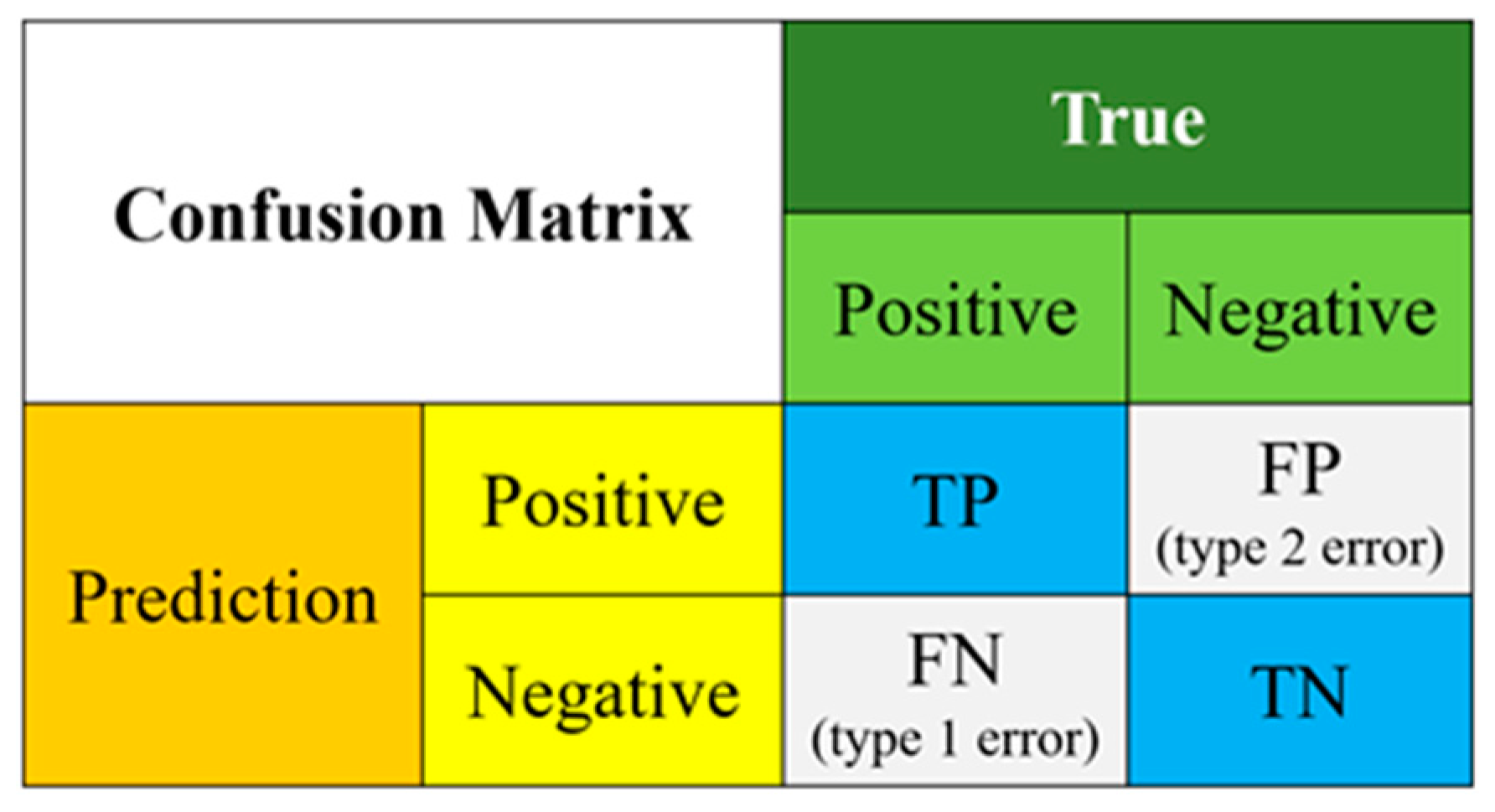
In the field of machine learning, the confusion matrix is the most intuitive indicator for judging the quality of a classification model and also the simplest two-classification method; see Figure 3. The final judgment type of the model was positive or negative. TP (True Positive) represented the number of samples where the true value and the predicted value were both positive. FN (False Negative) represents the number of samples where the true value was positive and the predicted value was negative. FP (False Positive) represents a sample where the true value and the predicted value were both negative. TN (True Negative) represents the number of samples whose true value was negative and predicted value was positive, where FN and FP are the first and second types of error. Theoretically, the larger the TP and TN, the more accurate the model, and the smaller the FP and FN, the better the performance [25,26].

The extended classification model performance indicators for the confusion matrix are as follows [25]:

• Accuracy: The proportion of the overall number of correct samples in the classification model to the total number of observed samples.

  $$Acc=\frac{TP+TN}{TP+FP+FN+TN}$$

  (18)
• Precision: Among all the results predicted by a certain category, the model predicts the correct proportion.

  $$Pre=\frac{TP}{TP+FP}$$

  (19)
• Sensitivity, also known as recall: The model predicts the correct proportion of all samples that are true for a certain category.

  $$Sen=\frac{TP}{TP+FN}$$

  (20)
• Specificity: Among all real samples outside a certain category, the model predicts the proportion of non-this category.

  $$Spe=\frac{TN}{TN+FP}$$

  (21)
• F1-Score: Integrates the results of accuracy and sensitivity to measure the quality of the output result in the range of 0~1. The closer to 1, the better the model, and the closer to 0, the worse the model.

  $$F1-Score=\frac{2\times TP}{2\times TP+FP+FN}=\frac{2\times \left(Pre\times Sen\right)}{Pre+Sen}$$

  (22)

3.3. Using the Maximum Lyapunov Exponent as a Prediction Index

In this study, the two parameters of damping and stiffness coefficients were within a range of 0.04~0.1 and 0~4. The data volume was 201. The parameter increment of damping and stiffness were 0.0003 and 0.0200. After the two parameters were combined, the data volume of the maximum Lyapunov exponent (MLE) was 201 × 201. The 201 × 201 dataset was used as the prediction target, and then datasets of 21 × 21, 51 × 51, and 101 × 101 were used as the training data volumes. Gaussian process regression (GPR) and backward propagation neural network (BPNN) were used for learning. In addition to comparing the prediction differences between GPR and BPNN, the effect of training with a small amount of data was also discussed.

4. Results and Discussion

4.1. Analysis of the Response of a Damping Coefficient to the System

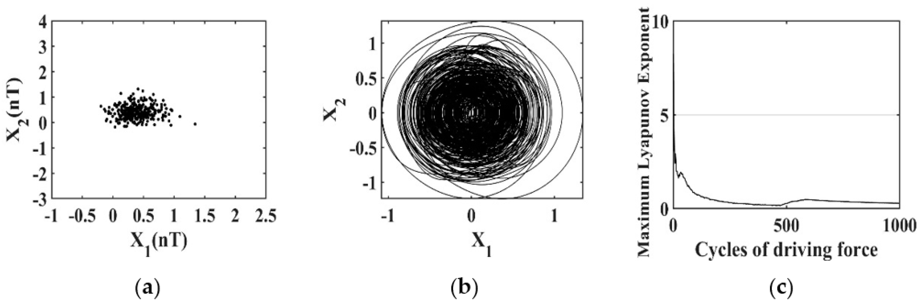
When the damping coefficient was set to U₀ = 0.04–0.1 and the stiffness parameter to N₂ = 0.2, and the increment of U₀ was 0.0003, there was a total yield of 201 dynamic orbit data, which could be used to calculate the phase portrait, Poincaré map, MLE, and bifurcation diagrams. The impact of U₀ on the dynamic behavior of the robotic system was analyzed and explored. The results (see Figure 4, Figure 5, Figure 6 and Figure 7) showed that system behavior was unstable and motion was asymmetric when U₀ = 0.0400–0.0451. At U₀ = 0.0841, there was a gradual approach to symmetrical stability. When U₀ = 0.0997, motion was stable, symmetric, and periodic. From the bifurcation diagram shown in Figure 8, it can be seen that U₀ gradually caused the system to become stable from 0.04–0.1. It was stable from U₀ = 0.0976–0.0994, but unstable when U₀ = 0.040–0.044.

The vibration behavior of the robotic arm system is complex, but it was clear that the higher the damping coefficient, the more obvious the periodic behavior. To further clarify the occurrence of non-periodic behavior and chaos, MLE was used to verify the phenomenon. Chaos occurs when MLE was greater than 0, as can be seen in Figure 4c and Figure 5c, and MLE can be used to compare and demonstrate the occurrence of chaos in the bifurcation diagram with the MLE distribution, as shown in Figure 9. It can be seen that the range of periodic behavior increased significantly when U₀ ≥ 0.08, although chaos still existed within some stable ranges. The dynamic behavior of the overall damping parameter is summarized in detail in

Table 2. Dynamic behavior for U₀ = 0.04–0.10.

$U_0$	(0.04, 0.0412)	(0.0412, 0.0415)	(0.0415, 0.0448)	(0.0448, 0.0451)
Dynamic behavior	chaos	T	chaos	T
$U_0$	(0.0451, 0.0457)	(0.0457, 0.0463)	(0.0463, 0.0490)	(0.0490, 0.0493)
Dynamic behavior	chaos	T	chaos	T
$U_0$	(0.0493, 0.0547)	(0.0547, 0.0550)	(0.0550, 0.0580)	(0.0580, 0.0583)
Dynamic behavior	chaos	T	chaos	T
$U_0$	(0.0583, 0.0610)	(0.0610, 0.0613)	(0.0613, 0.1]
Dynamic behavior	chaos	T	Chaos and T appear interactively

.

4.2. Analysis of the Response of Stiffness to the System

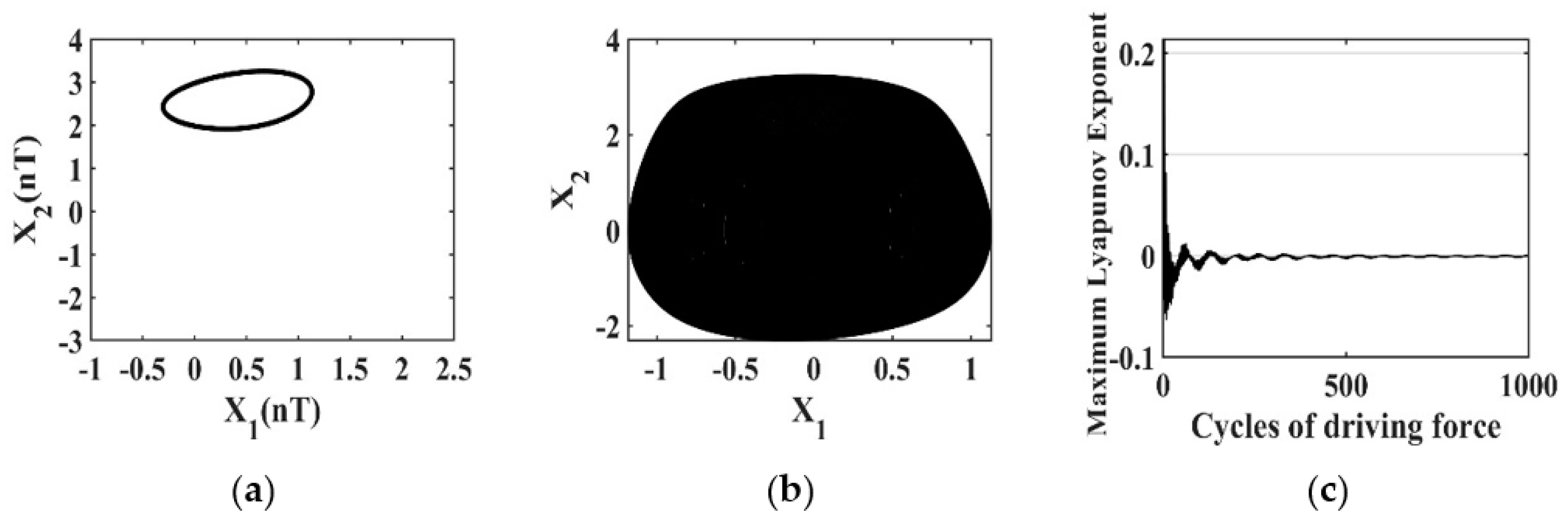
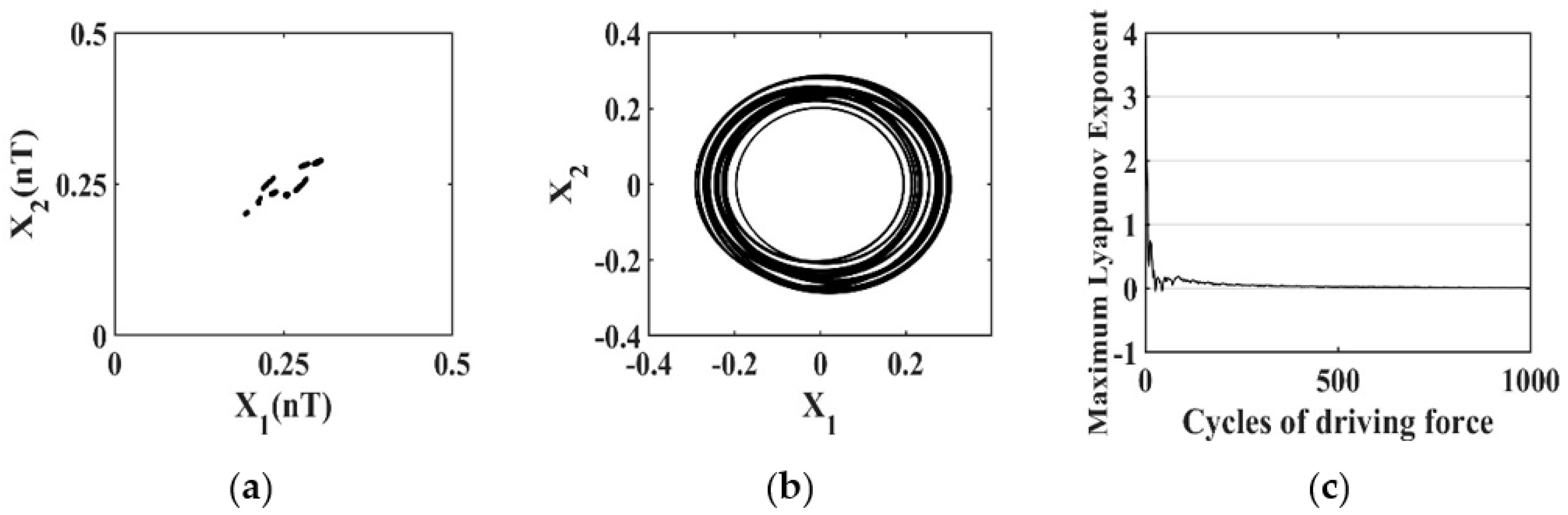
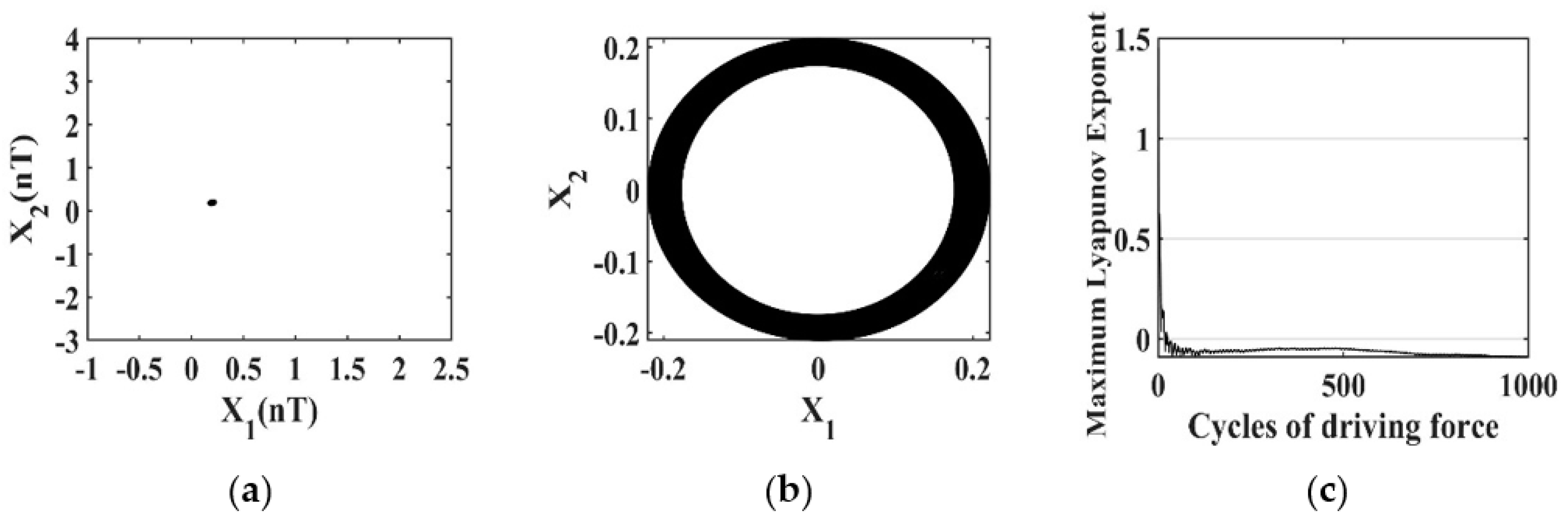
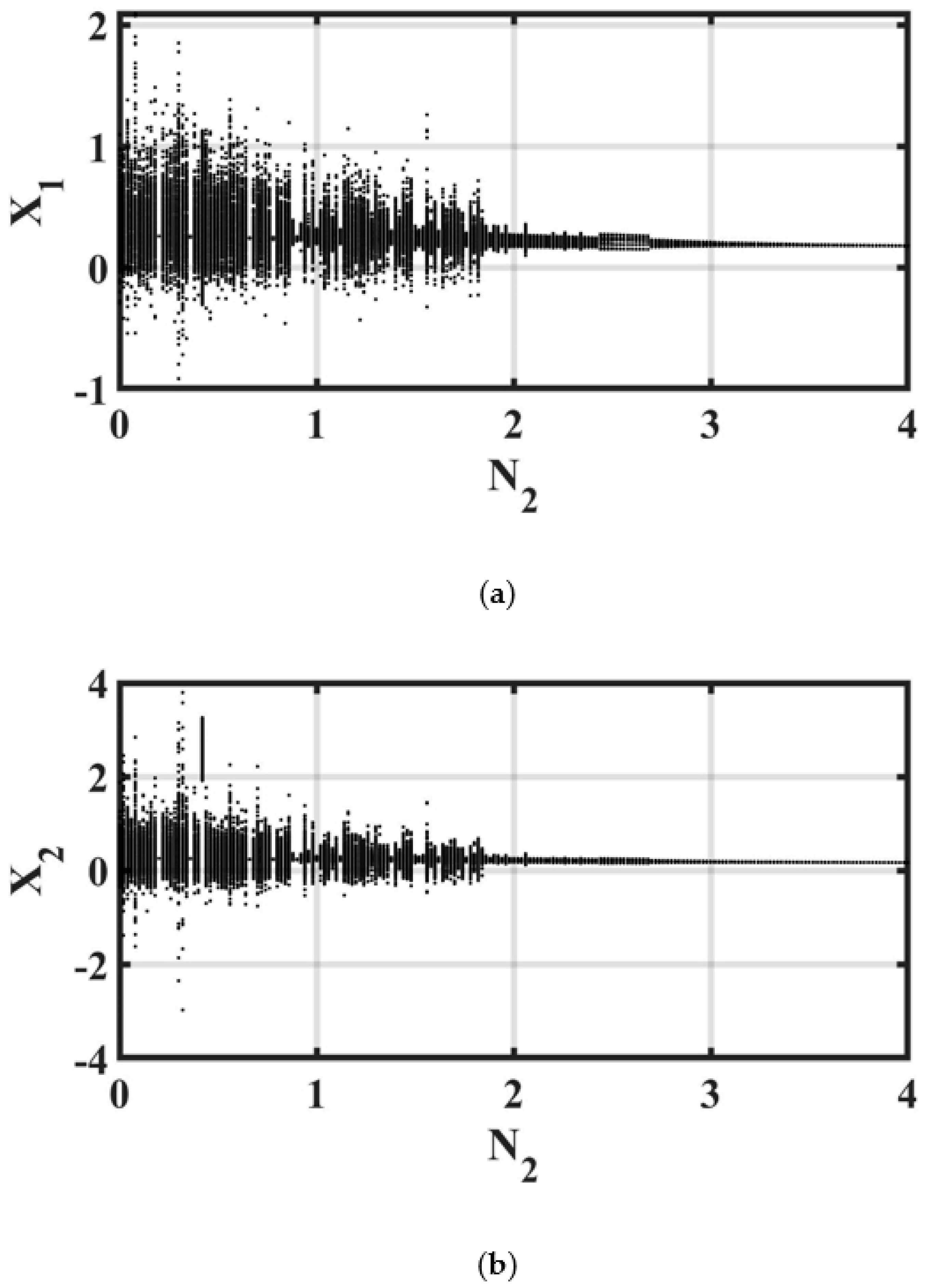
The stiffness coefficient, N₂, was set to within a range of 0 to 4.0 with damping U₀ = 0.0418, and the N₂ increment used was 0.05, and the yield was a set of 201 data, the same as U₀. From Figure 10, Figure 11, Figure 12, Figure 13 and Figure 14, it can be seen that unstable and asymmetric motion occurred when N₂ = 0.24, 0.42 and symmetric stability was gradually approached as N₂ = 1.38, 2.44. When N₂ = 2.84, behavior was stable, symmetrical, and periodic. From the bifurcation diagram shown in Figure 15, it can be seen that the unstable state occurred over the range of N₂ = 0 to 1.5. It can be observed from the bifurcation phenomenon that the nonlinear aperiodic behavior was obvious in the interval of N₂ < 2.08, and the higher the stiffness, the more obvious the periodic behavior. When N₂ > 2.08, periodic motion replaced unstable nonlinear motion shown in Figure 16.

The chaotic behavior of the system was also verified by MLE, as can be seen in Figure 10c, Figure 11c, Figure 12c, Figure 13c and Figure 14c, and it was clear that chaos occurred at N₂ = 0.24 with MLE greater than 0. When N₂ ≥ 2.08 and MLE were less than or equal to 0, the system behavior was non-chaotic. This was consistent with the bifurcation diagram and the detailed dynamic behavior changes with N₂, as shown in

Table 3. Dynamic behavior of N₂ = 0~4.0.

$N_2$	(0.00, 0.20)	(0.20, 0.22)	(0.22, 0.36)	(0.36, 0.38)	(0.38, 0.42)
Dynamic behavior	chaos	T	chaos	T	chaos
$N_2$	(0.42, 0.44)	(0.44, 0.66)	(0.66, 0.68)	(0.68, 0.78)	(0.78, 0.80)
Dynamic behavior	quasi-period	chaos	T	chaos	T
$N_2$	(0.80, 0.90)	(0.90, 0.92)	(0.92, 1.38)	(1.38, 1.40)	(1.40, 2.00)
Dynamic behavior	chaos	T	chaos	multi-period	chaos
$N_2$	(2.00, 2.06)	(2.06, 2.08)	(2.08, 2.38)	(2.38, 2.42)	(2.42, 2.44)
Dynamic behavior	quasi-period	chaos	quasi-period	multi-period	quasi-period
$N_2$	(2.44, 2.70)	(2.70, 2.84)	(2.84, 4.00)
Dynamic behavior	5T	quasi-period	T

.

4.3. Image Recognition Results

The phase portrait and Poincaré map were used to perform image recognition experiments. The following results demonstrate the recognition effects by GoogLeNet and ResNet-50; the training accuracy and confusion matrix using the same settings and datasets were also compared.

4.3.1. Image Recognition of Phase Portraits

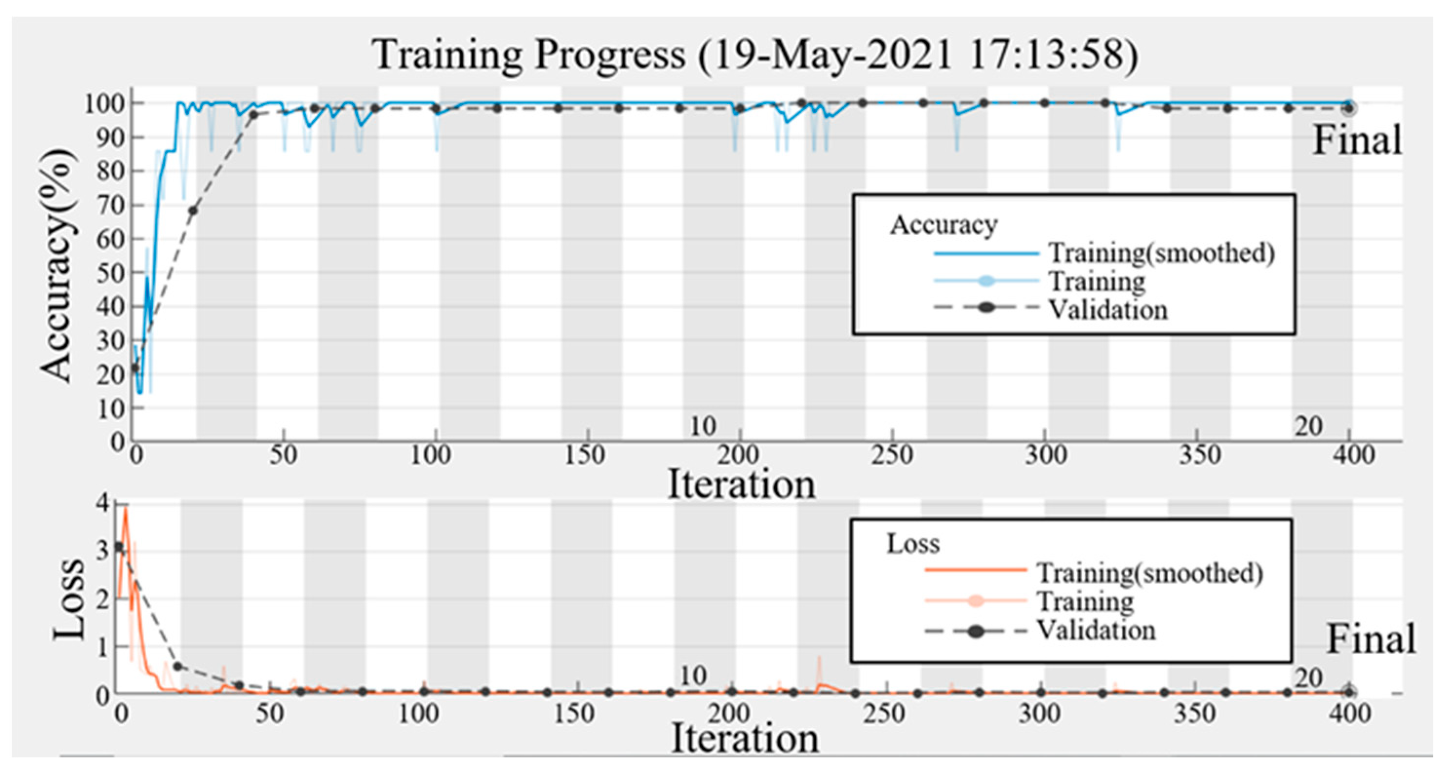
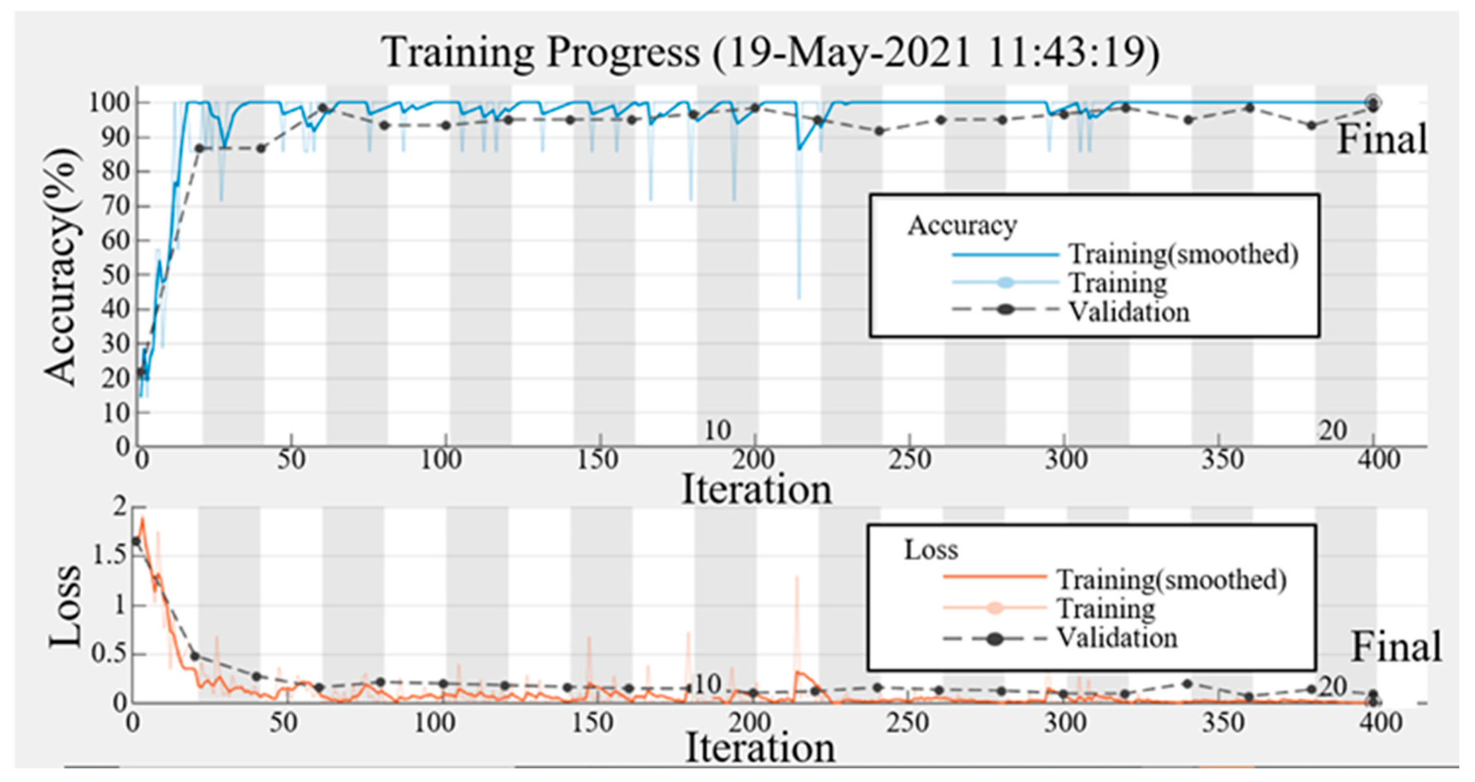
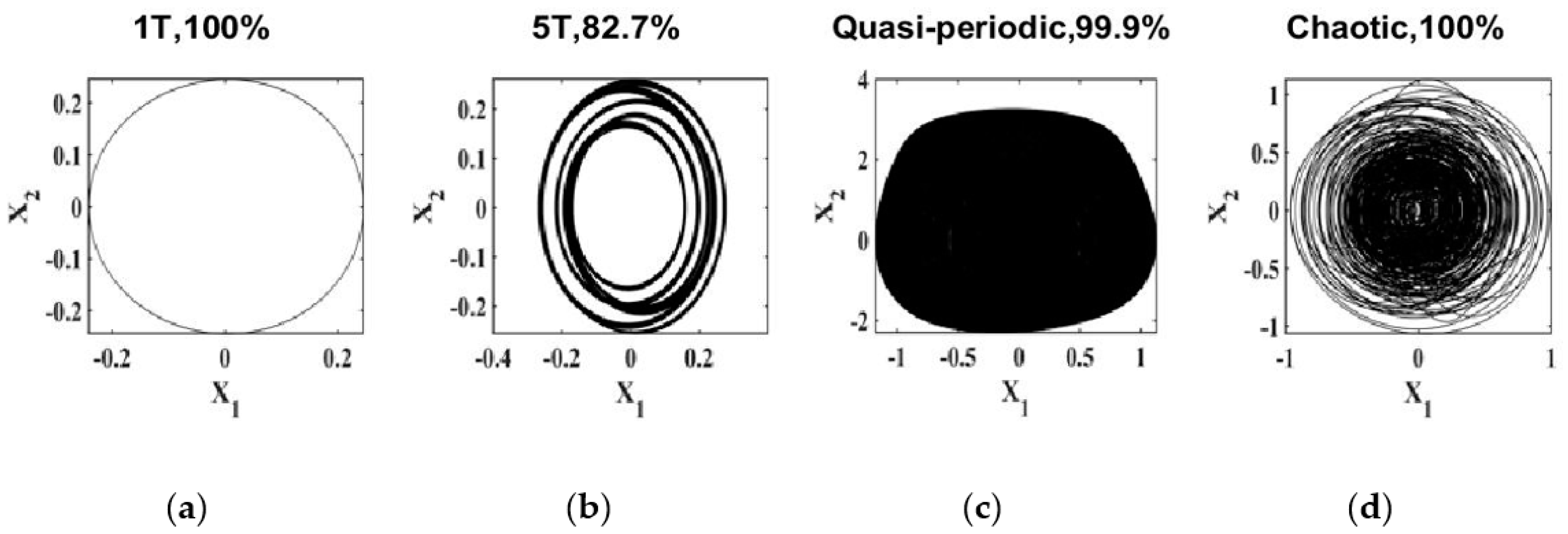
The training accuracy and loss curves of GoogLeNet and ResNet-50 with 200 phase portraits as learning samples are shown in Figure 17 and Figure 18. Accuracy increases during the training process and losses decrease for both GoogLeNet and ResNet-50. However, it can be clearly seen that GoogLeNet performs better with respect to convergence. In the final epoch, the verification accuracy of ResNet-50 (100%) was slightly higher than that of GoogLeNet (98.33%); see

Table 4. Phase portrait Training Results.

Item	Details	GoogLeNet	ResNet-50
Results	Validation accuracy	98.33%	100%
Training Time	Elapsed time	40 min 11 s	69 min 41 s
Training Cycle	Epoch	20 of 20
	Iteration	400 of 400
	Iterations per epoch	20
	Maximum iterations	400
Validation	Frequency	20 iterations
Other Information	Hardware resource	Single CPU
	Learning rate	0.0001

. Figure 19 and Figure 20 show the identification results and probability of four kinds of dynamic phase portrait from 600 images of the original dataset. It can be seen that the rate of identification by GoogLeNet was higher than that of ResNet-50. However, it was necessary to compare the performance of the two models with a confusion matrix and to evaluate classification model performance. Examination of Figure 21 shows that, although the identification accuracy of GoogLeNet was as high as 99.5% using the original dataset of 600 samples, the identification accuracy of ResNet-50, where all categories are correctly identified, was 100%. In

Table 5. Comparison of various performance indicators of phase portrait identification with GoogLeNet and ResNet-50.

Type	Indicator	GoogLeNet	ResNet-50
1T	Precision	1	1
	Sensitivity	0.98	1
	Specificity	1.007	1
	F1-Score	0.99	1
5T	Precision	1	1
	Sensitivity	1	1
	Specificity	1	1
	F1-Score	1	1
Quasi-periodic	Precision	0.98	1
	Sensitivity	1	1
	Specificity	0.993	1
	F1-Score	0.99	1
Chaotic	Precision	1	1
	Sensitivity	1	1
	Specificity	1	1
	F1-Score	1	1
Accuracy		0.995	1

, a comparison of identification of the phase portraits made by the two applications shows that ResNet-50 was better than GoogLeNet for 1T and quasi-period identification, and was also better in terms of overall performance.

4.3.2. Image Recognition of Poincaré Map

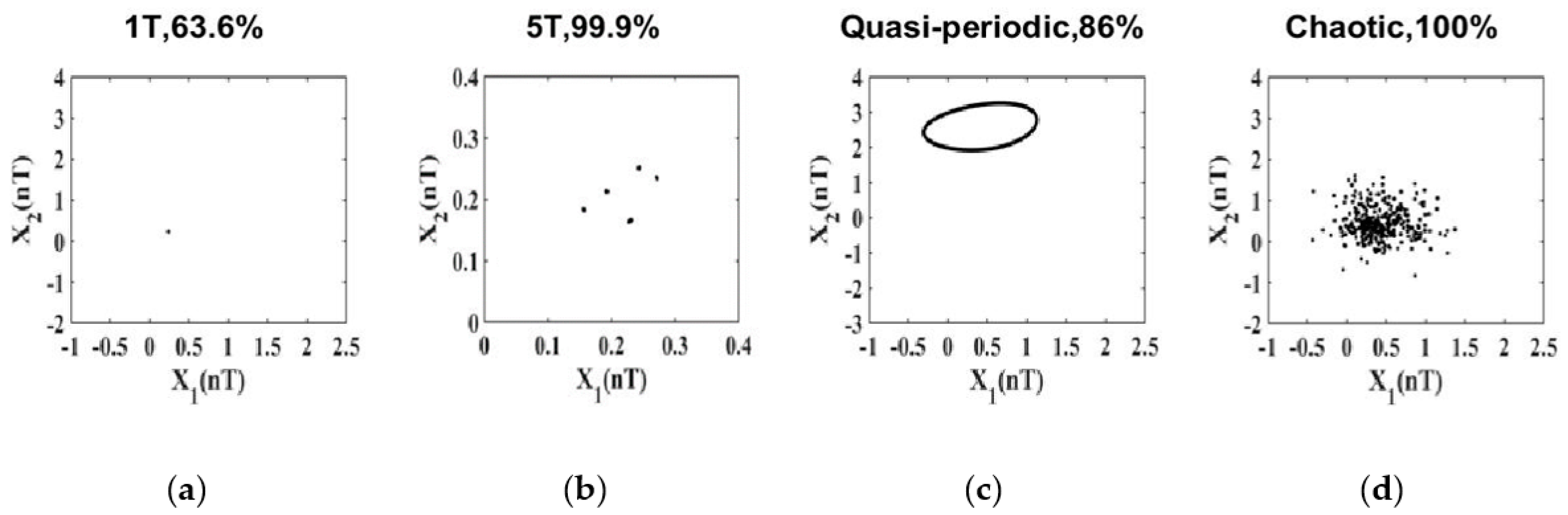
The training accuracy and loss curves of GoogLeNet and ResNet-50 with 200 Poincaré map learning samples are shown in Figure 22 and Figure 23. It can be clearly seen that, during training, convergency was better with GoogLeNet than with esNet-50. Additionally, the GoogLeNet verification accuracy of 98.33% was higher than that of ResNet-50 at 95%; see

Table 6. Training Results of Poincaré map.

Item	Details	GoogLeNet	ResNet-50
Results	Validation accuracy	98.33%	95.00%
Training Time	Elapsed time	18 min 34 s	86 min 19 s
Training Cycle	Epoch	20 of 20
	Iteration	400 of 400
	Iterations per epoch	20
	Maximum iterations	400
Validation	Frequency	20 iterations
Other Information	Hardware resource	Single CPU
	Learning rate	0.0001

. The identification results and probability of four kinds of Poincaré map from 600 original dataset images are shown in Figure 24 and Figure 25. It can be seen that the rate of identification by GoogLeNet was higher than by ResNet-50, and the tendency was the same as that seen in phase portrait identification. The confusion matrix was also used to evaluate the performance of the compared models. Figure 26 shows that identification, also using the original dataset, was 97.2% for GoogLeNet and 98.8% for ResNet-50.

Table 7. Comparison of various performance indicators of Poincaré map identification with GoogLeNet and ResNet-50.

Type	Indicator	GoogLeNet	ResNet-50
1T	Precision	0.993	1
	Sensitivity	0.94	1
	Specificity	1.018	1
	F1-Score	0.966	1
5T	Precision	0.942	1
	Sensitivity	0.98	0.967
	Specificity	0.987	1.011
	F1-Score	0.961	0.983
Quasi-periodic	Precision	1	0.974
	Sensitivity	0.967	0.987
	Specificity	1.011	0.996
	F1-Score	0.983	0.98
Chaotic	Precision	0.955	0.98
	Sensitivity	1	1
	Specificity	0.984	0.993
	F1-Score	0.977	0.99
Accuracy		0.972	0.988

shows a comparison of GoogLeNet and ResNet-50 performance Poincaré map identification indicators. It can be seen that only the quasi-period motion identification by GoogLeNet was better than that of ResNet-50. The conclusion was that, in terms of overall performance, ResNet-50 was better than GoogLeNet.

4.4. Forecast Results of the Maximum Lyapunov Exponent

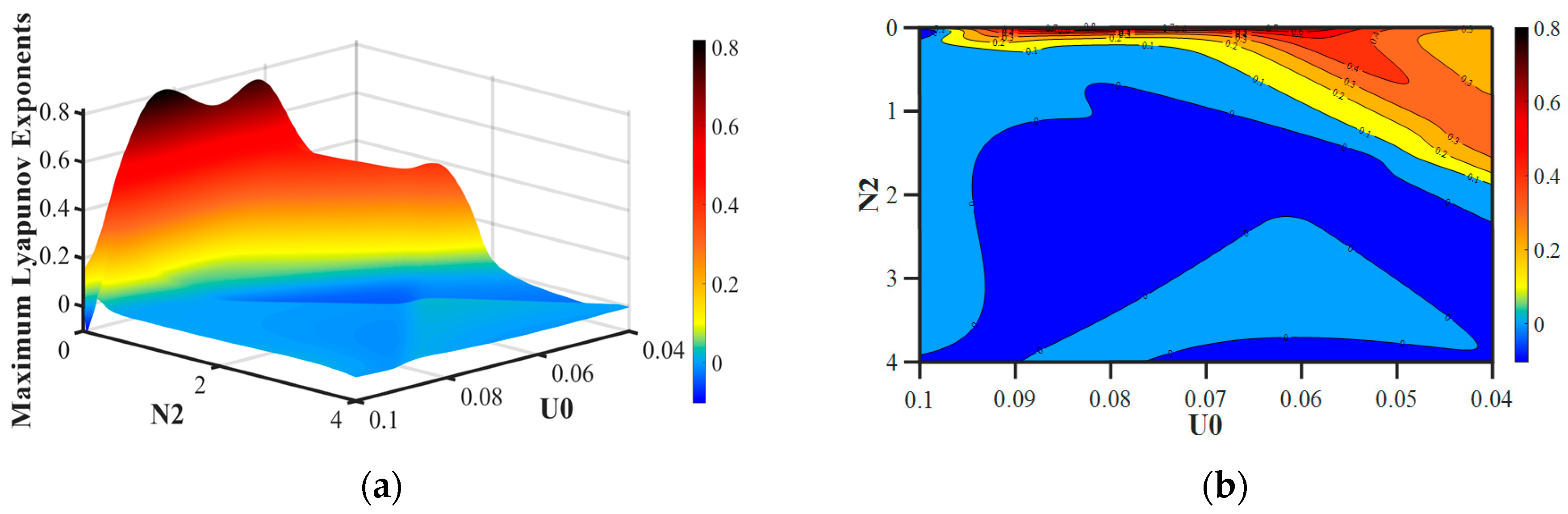
In this section, the prediction effects of Gaussian process regression and the backward propagation neural network are discussed as well as the observed prediction with different amounts of data. Four indicators were used to compare the training error in different situations and the prediction error using the original dataset; see Figure 27.

4.4.1. Prediction by Gaussian Process Regression (GPR)

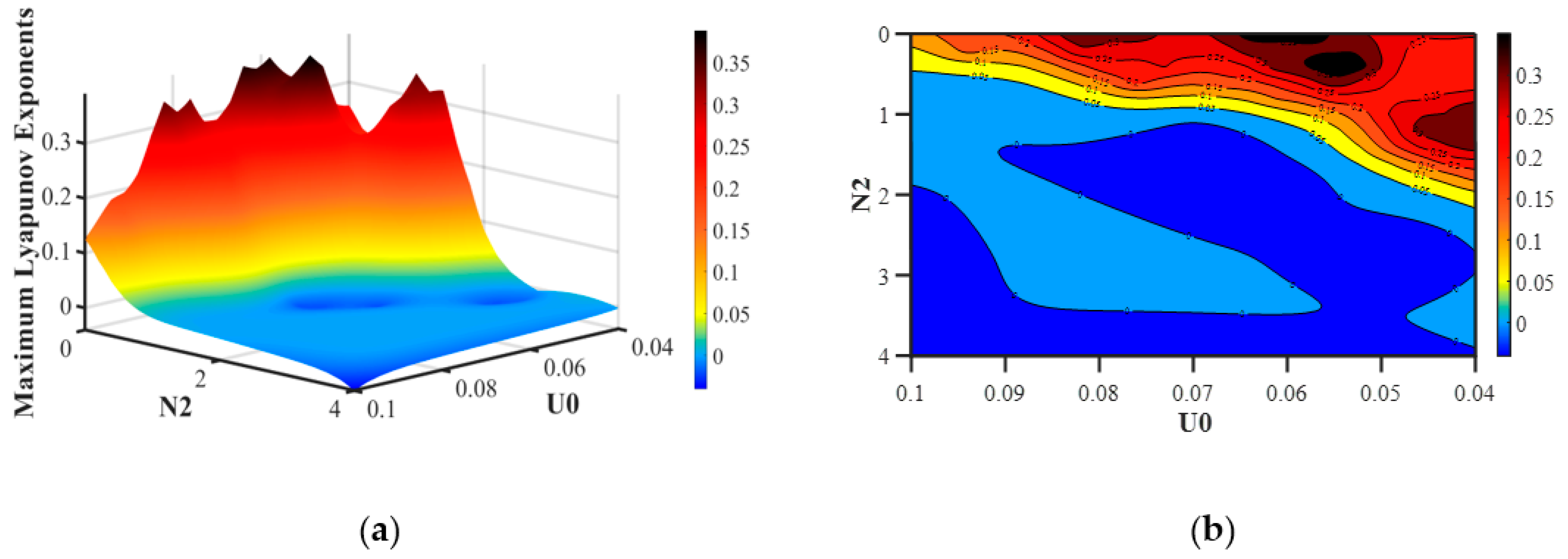
Figure 28, Figure 29 and Figure 30 show the MLE results predicted by the GPR model with training data volumes of 21 × 21, 51 × 51, and 101 × 101. If MLE was greater than zero, the system was chaotic, and ranges from yellow to red are shown on the graph. When the MLE was less than or equal to zero, behavior was non-chaotic (1T, 5T, and quasi-periodic motion) and is shown as light green to dark blue on the graph. A comparison of Figure 30, Figure 31 and Figure 32 with Figure 29 shows that the results predicted by different amounts of data differ slightly, but most of the distribution ranges of chaotic and periodic intervals could be predicted. However, some periodic behavior occurred within the chaotic area, and then accurate prediction was difficult. There was also a gap between the highest point of the predicted index and the real situation. These two phenomena may have been caused by overfitting in the training process.

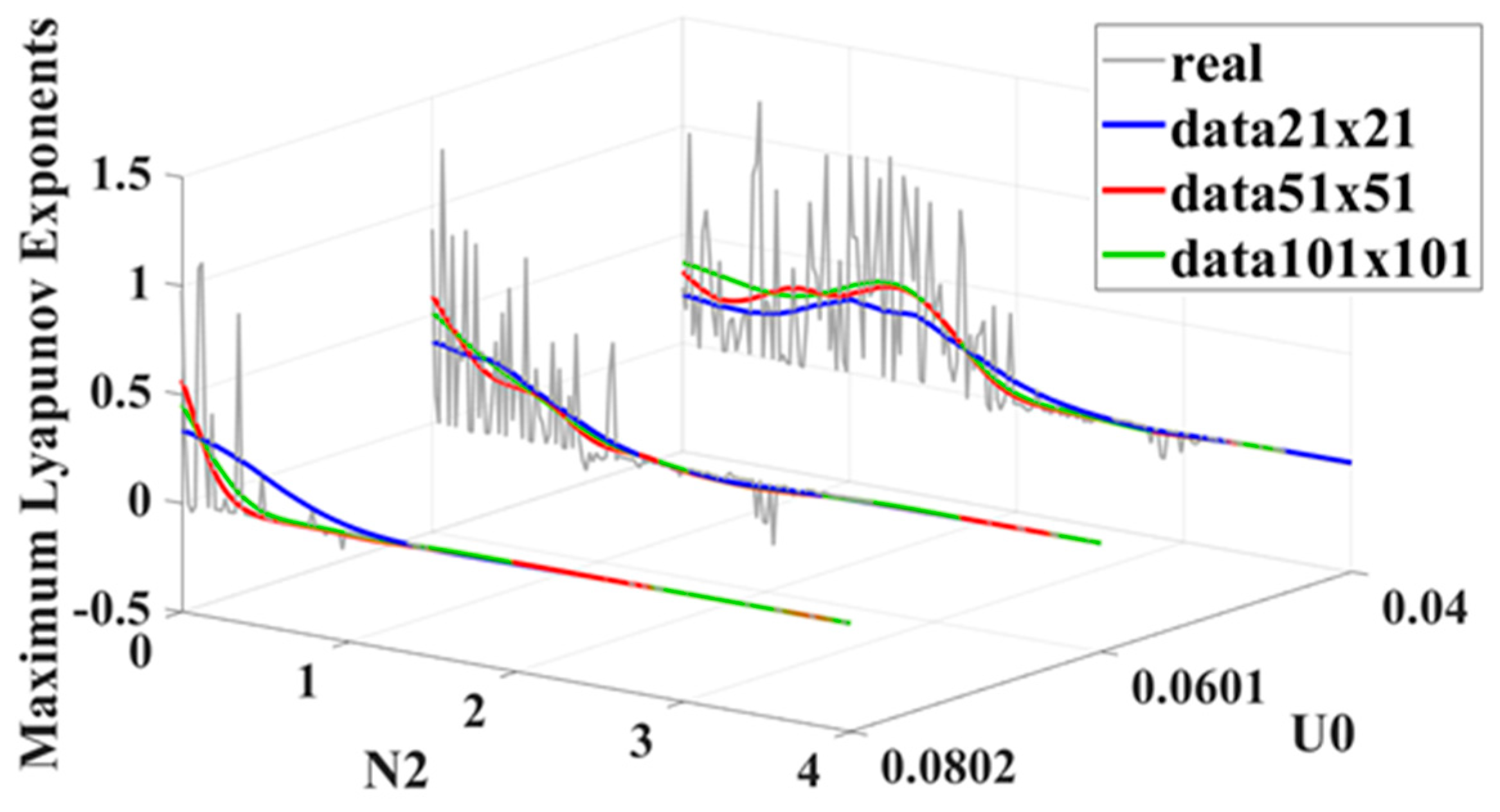
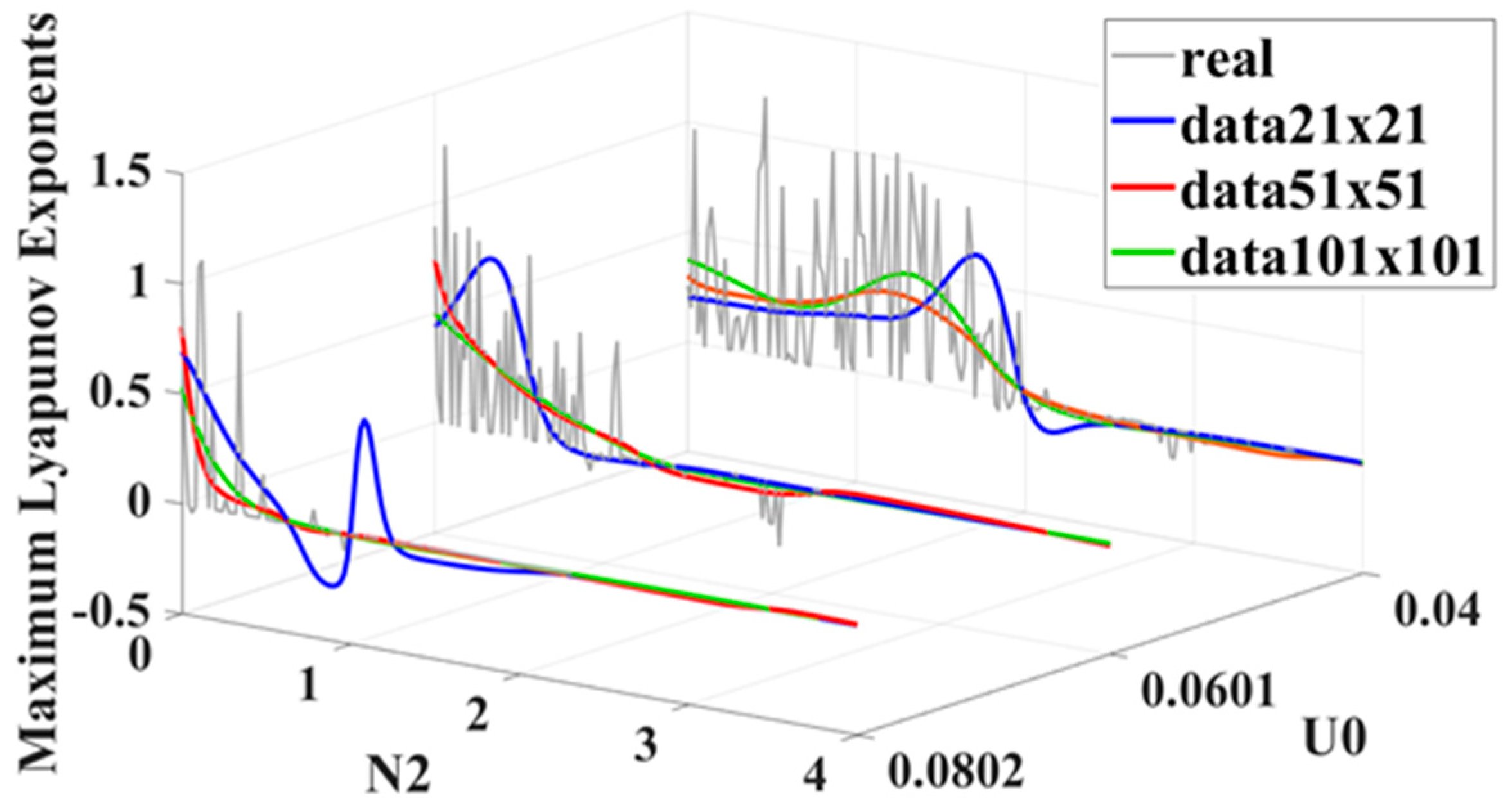
Comparisons of predictions were made with three different amounts of training dataset, as shown in Figure 31. Three values of damping coefficient, 0.0400, 0.0601, and 0.0802, were used in stiffness prediction; see the figure. It was found that if the highest point of the MLE had been predicted, the 51 × 51 and 101 × 101 dataset predictions were closer to the real value than those of the 21 × 21 dataset. The distribution of chaos and periodic motion for all three datasets could be predicted as approaching zero with an MLE less than zero. The predicted results did not affect the interpretation of periodic behavior, and the three predictions for periodic behavior were all excellent. However, it was clear that the 21 × 21 training dataset predicted more chaotic behavior than the other two. This was confirmed by observation that the area of chaos predicted was significantly larger than in the other two; see the contour maps in Figure 28b, Figure 29b and Figure 30b.

4.4.2. Prediction by Backward Propagation Neural Network Prediction (BPNN)

Figure 32, Figure 33 and Figure 34 show the results of BPNN predictions with training data volumes of 21 × 21, 51 × 51, and 101 × 101. Areas that appear from yellow to red on the graphs represent chaotic motion and those from light green to dark blue represent periodic behavior. A comparison with real values is shown in Figure 31. While it is obvious that the 51 × 51 and 101 × 101 prediction results differ slightly from one another, they do predict most of the range of chaos and periodic motion distribution. However, none of the datasets predicted the existence of the few areas of periodic behavior within the chaotic interval. This may be the result of overfitting, as seen in the GPR model.

Figure 35 shows a comparison of the changes in the stiffness curve with three different damping values, 0.0400, 0.0601, and 0.0802. The 21 × 21 dataset comes closest to a prediction of the real maximum value of MLE, followed by 51 × 51. However, when it comes to a prediction of the distribution of chaos and periodic motion, the 21 × 21 data training set has a problem. In light of this, only the other two will be given consideration.

Both the 51 × 51 and 101 × 101 datasets could correctly predict values for the MLE. However, with damping values between 0.0400 and 0.0802, the 101 × 101 training result was much better at the prediction of chaotic behavior than the 51 × 51 dataset and predicted far more chaotic intervals. A comparison of the contour maps confirmed that the area of chaotic behavior predicted by 101 × 101 was significantly larger than that of the 51 × 51 dataset; see Figure 33b and Figure 34b.

4.4.3. Comparison of Gaussian Process Regression and the Backward Propagation Neural Network

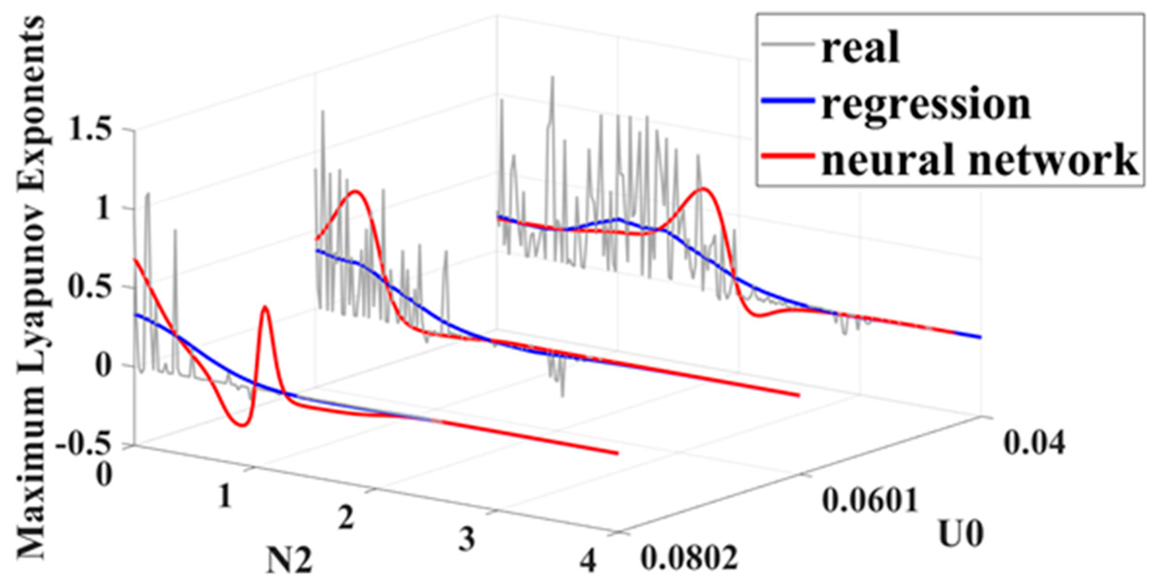
GPR has obvious prediction advantages in respect to the 21 × 21 dataset because BPNN predicts part of the chaos to be periodic motion; see the red lines in Figure 36. However, the prediction results for 51 × 51 and 101 × 101 for both GPR and BPNN were similar, as can be seen in Figure 37 and Figure 38. It was clear that there were training errors in these two prediction models, and they are listed in

Table 8. A comparison of GPR and BPNN training.

Method	Data	RMSE	R2	MSE	MAE
GPR	21 × 21	0.1669	0.34	0.0279	0.0852
	51 × 51	0.1454	0.45	0.0211	0.0610
	101 × 101	0.1584	0.37	0.0251	0.0655
BPNN	21 × 21	0.1769	0.28	0.0313	0.0846
	51 × 51	0.1532	0.41	0.0235	0.0729
	101 × 101	0.1587	0.38	0.0252	0.0655

and

Table 9. Comparison of prediction errors between GPR and BPNN with the original dataset 201 × 201.

Method	Data	RMSE	R2	MSE	MAE
GPR	21 × 21	0.1644	0.32	0.0270	0.0714
	51 × 51	0.1619	0.34	0.0262	0.0642
	101 × 101	0.1603	0.35	0.0257	0.0649
BPNN	21 × 21	0.1978	0.01	0.0391	0.0859
	51 × 51	0.1644	0.32	0.0270	0.0684
	101 × 101	0.1605	0.35	0.0257	0.0657

. After a comprehensive analysis of the various indicators and a comparison of training errors, it was found that both models had their best effect with the 51 × 51 dataset training. However, GPR had fewer errors than BPNN. Both prediction models reached their lowest prediction error rate with the 101 × 101 dataset, but the GPR error rate was lower than that of BPNN. It is worth mentioning that the GPR-21 × 21 model was actually quite compatible with the BPNN-51 × 51 model in terms of error and determination coefficients. However, data analysis and examination of the graphs showed GPR prediction to be superior to that of BPNN.

5. Conclusions

In this study, the nonlinear dynamics of a robotic arm system were simulated, and a variety of dynamic behaviors including periodic symmetry, subharmonic, quasi-periodic, and chaotic motion were analyzed. After verification, chaotic and non-chaotic behavior could be distinguished using bifurcation diagrams and MLE. The results showed that the higher the value of the damping and stiffness coefficients, the better the stability. The best chance of robot system stability was achieved when the damping coefficient was controlled between 0.0796 and 0.100 (avoiding the range of 0.0400 to 0.0796) and the stiffness coefficient was set between 2.08 to 4.00 (avoiding a range of <2.08). Both GoogLeNet and ResNet-50 gave good recognition results, but ResNet-50 gave better graphics recognition performance than GoogLeNet. This was especially so for the accuracy of recognition of the phase portrait and Poincaré map. ResNet-50 results for these were 0.5% and 1.6% higher than those of GoogLeNet. It was also shown that a small amount of training data can be used to obtain excellent prediction results. The time taken to obtain a 101 × 101 dataset was 3.92 times that for 21 × 21, so both cost and training time can be greatly reduced. The only really serious error found in a comparison of GPR and BPNN prediction results was a clear trend in BPNN-21 × 21 towards the prediction of chaos as periodic motion. It is recommended that GPR be used for higher reliability when only a small sample of data is available for training. The results also showed that the smallest training error values were achieved using the 101 × 101 dataset. GPR had smaller model training errors than BPNN on the three types of data, and GPR prediction was better than BPNN for the robotic arm system chosen for this study.

These results can be applied and implemented for the multi-axis robotic arms widely used in automobile and component manufacture, as well as in many electronics related industries. Increased precision allows better movement in three-dimensional space as well as in linear displacement. The identification and prediction of results can be used to inhibit nonlinear vibration in robotic arms, improve accuracy, and reduce positioning errors as the arm moves. The results can also be used as guidelines for future research for the saving of costs and the reduction of production time and manpower spent on quality control in modern manufacturing.

References

- Futami, S.; Kyura, N.; Hara, S. Vibration absorption control of industrial robots by acceleration feedback. IEEE Trans Ind. Electron. 1983, 3, 299–305. [Google Scholar] [CrossRef]
- Jam, J.; Fard, A.A. Application of single unit impact dampers to reduce undesired vibration of the 3R robot arms. Int. Aerosp. Sci. 2013, 2, 49–54. [Google Scholar]
- Goswami, A.; Thuilot, B.; Espiau, B. A study of the passive gait of a compass-like biped robot: Symmetry and chaos. Int. J. Rob. Res. 1998, 17, 1282–1301. [Google Scholar] [CrossRef]
- Lankalapalli, S.; Ghosal, A. Possible chaotic motions in a feedback controlled 2R robot. Proc. IEEE Int. Conf. Rob. Autom. 1996, 2, 1241–1246. [Google Scholar]
- Lankalapalli, S.; Ghosal, A. Chaos in robot control equations. Int. J. Bifurc. Chaos 1997, 7, 707–720. [Google Scholar] [CrossRef]
- Sado, D.; Gajos, K. Note on chaos in three degree of freedom dynamical system with double pendulum. Meccanica 2003, 38, 719–729. [Google Scholar] [CrossRef]
- Tolgay, K.; Ali, M. Adaptive PD-SMC for nonlinear robotic manipulator tracking control. Stud. Inf. Control. 2017, 26, 49–58. [Google Scholar] [CrossRef] [Green Version]
- Razzaghi, P.; Khatib, E.A.; Hurmuzlu, Y. Nonlinear dynamics and control of an inertially actuated jumper robot. Nonlinear Dyn. 2019, 97, 161–176. [Google Scholar] [CrossRef]
- Mustafa, M.; Hamarash, I.; Crane, C.D. Dedicated nonlinear control of robot manipulators in the presence of external vibration and uncertain payload. Robotics 2020, 9, 2. [Google Scholar] [CrossRef] [Green Version]
- Dachang, Z.; Baolin, D.; Puchen, Z.; Wu, W. Adaptive backstepping sliding mode control of trajectory tracking for robotic manipulators. Complexity 2020, 2020, 3156787. [Google Scholar] [CrossRef]
- Xu, Y.; Zhou, Y.; Sekula, P.; Ding, L. Machine learning in construction: From shallow to deep learning. Dev. Built Environ. 2021, 6, 100045. [Google Scholar] [CrossRef]
- Praveenkumar, T.; Saimurugan, M.; Krishnakumar, P.; Ramachandran, K. Fault diagnosis of auto- mobile gearbox based on machine learning techniques. Procedia Eng. 2014, 97, 2092–2098. [Google Scholar] [CrossRef] [Green Version]
- Mohandes, M.A.; Halawani, T.O.; Rehman, S.; Hussain, A.A. Support vector machines for wind speed prediction. Renew. Energy 2004, 29, 939–947. [Google Scholar] [CrossRef]
- Altay, O.; Gurgenc, T.; Ulas, M.; Özel, C. Prediction of wear loss quantities of ferro-alloy coating using different machine learning algorithms. Friction 2020, 8, 107–114. [Google Scholar] [CrossRef] [Green Version]
- Wang, G.; Qian, L.; Guo, Z. Continuous tool wear prediction based on Gaussian mixture regression model. Int. J. Adv. Manu. Technol. 2013, 66, 1921–1929. [Google Scholar] [CrossRef]
- Geetha, N.; Bridjesh, P. Overview of machine learning and its adaptability in mechanical engineering. Mater. Today Proc. 2020. [Google Scholar] [CrossRef]
- Talo, M. Automated classification of histopathology images using transfer learning. Artif. Intell. Med. 2019, 101, 101743. [Google Scholar] [CrossRef] [Green Version]
- Chen, J.; Chen, J.; Zhang, D.; Sun, Y.; Nanehkaran, Y.A. Using deep transfer learning for image-based plant disease identification. Comput. Electron Agric. 2020, 173, 105393. [Google Scholar] [CrossRef]
- Szegedy, C.; Liu, W.; Jia, Y.; Sermanet, P.; Reed, S.; Anguelov, D.; Erhan, D.; Vanhoucke, V.; Rabinovich, A. Going deeper with convolutions. In Proceedings of the IEEE Conference on Computer Vision and Pattern Recognition (CVPR), Boston, MA, USA, 7–12 June 2015; pp. 1–9. [Google Scholar] [CrossRef] [Green Version]
- Marei, M.; Zaatari, S.E.; Li, W. Transfer learning enabled convolutional neural networks for estimating health state of cutting tools. Rob. Comput. Integ. Manuf. 2021, 71, 102145. [Google Scholar] [CrossRef]
- Hashemi, S.M.; Werner, H. Parameter identification of a robot arm using separable least squares technique. In Proceedings of the 2009 European Control Conference (ECC), Budapest, Hungary, 23–26 August 2009; pp. 2199–2204. [Google Scholar]
- Sabine, H.; Hans, N. System identification of a robot arm with extended Kalman filter and artificial neural networks. J. Appl. Geod. 2019, 13, 135–150. [Google Scholar] [CrossRef]
- Cheong, J.; Aoustin, Y.; Bidaud, P.; Noël, J.P.; Garnier, H.; Janot, A.; Carrillo, F. Identification of Rigid Industrial Robots A System Identification Perspective, Soutenance de These—Mathieu Brunot, 30 Novembre 2017 à 10h00. Available online: https://core.ac.uk/download/pdf/163105211.pdf (accessed on 30 November 2017).
- Felix, J.L.P.; Silva, E.L.; Balthazar, J.M.; Tusset, A.M.; Bueno, A.M.; Brasil, R.M.L.R.F. On nonlinear dynamics and control of a robotic arm with chaos. In Proceedings of the 2014 International Conference On Structural Nonlinear Dynamics And Diagnosis, Agadir, Morocco, 19–21 May 2014; Volume 16, pp. 1–6. [Google Scholar]
- Ahmad, A.; Saraswat, D.; Aggarwal, V.; Etienne, A.; Hancock, B. Performance of deep learning models for classifying and detecting common weeds in corn and soybean production systems. Comput. Electron. Agric. 2021, 184, 106081. [Google Scholar] [CrossRef]
- Madhavan, J.; Salim, M.; Durairaj, U.; Kotteeswaran, R. Wheat seed classification using neural network pattern recognizer. Mater. Today Proc. 2021, in press. [Google Scholar] [CrossRef]
Figure 1.
Schematic diagram of the robotic arm system.
Figure 2.
Flow chart.
Figure 3.
Schematic diagram of confusion matrix.
Figure 4.
Dynamic behavior for U0 = 0.04: (a) Poincaré map, (b) phase portrait, (c) maximum Lyapunov exponent.
Figure 5.
Dynamic behavior for U0 = 0.0451: (a) Poincaré map, (b) phase portrait, (c) maximum Lyapunov exponent.
Figure 6.
Dynamic behavior for U0 = 0.0841: (a) Poincaré map, (b) phase portrait, (c) maximum Lyapunov exponent.
Figure 7.
Dynamic behavior for U0 = 0.0997: (a) Poincaré map, (b) phase portrai, (c) maximum Lyapunov exponent.
Figure 8.
Bifurcation diagram of (a) displacement and (b) velocity of the damping coefficient on the robotic arm system.
Figure 9.
The distribution of the maximum Lyapunov exponent with different damping coefficients.
Figure 10.
Dynamic behavior for N2 = 0.24: (a) Poincaré map, (b) phase portrait, (c) maximum Lyapunov exponent.
Figure 11.
Dynamic behavior for N2 = 0.42: (a) Poincaré map, (b) phase portrait, (c) maximum Lyapunov exponent.
Figure 12.
Dynamic behavior for N2 = 1.38: (a) Poincaré map, (b) phase portrait, (c) maximum Lyapunov exponent.
Figure 13.
Dynamic behavior for N2 = 2.44: (a) Poincaré map, (b) phase portrait, (c) maximum Lyapunov exponent.
Figure 14.
Dynamic behavior for N2 = 2.84: (a) Poincaré map, (b) phase portrait, (c) maximum Lyapunov exponent.
Figure 15.
Bifurcation diagram of (a) displacement and (b) velocity of the stiffness coefficient on the robotic arm system.
Figure 16.
The distribution of the maximum Lyapunov exponent with different stiffness coefficient.
Figure 17.
Analysis of the training accuracy and loss status of the phase portrait using GoogLeNet.
Figure 18.
Analysis of the training accuracy and loss status of the phase portrait using ResNet-50.
Figure 19.
The identification of the phase portrait by GoogLeNet: (a) 1T, (b) 5T, (c) Quasi-periodic, (d) Chaotic.
Figure 20.
The identification of the phase portrait by ResNet-50: (a) 1T, (b) 5T, (c) Quasi-periodic, (d) Chaotic.
Figure 21.
Confusion matrix for phase image identification using (a) GoogLeNet and (b) ResNet-50.
Figure 22.
Analysis of the training accuracy and loss status of Poincaré map using GoogLeNet.
Figure 23.
Analysis of the training accuracy and loss status of Poincaré map using ResNet-50.
Figure 24.
Recognition of the Poincaré map using GoogLeNet: (a) 1T, (b) 5T, (c) Quasi-periodic, (d) Chaotic.
Figure 25.
Recognition of the Poincaré map using ResNet-50: (a) 1T, (b) 5T, (c) Quasi-periodic, (d) Chaotic.
Figure 26.
Confusion matrix for Poincaré map identification using (a) GoogLeNet and (b) ResNet-50.
Figure 27.
The original data distribution of the maximum Lyapunov exponent: (a) 3-Dimensional map, (b) contour map.
Figure 28.
Gaussian process regression prediction results (data 21 × 21): (a) 3-Dimensional map, (b) contour map.
Figure 29.
Gaussian process regression prediction results (data 51 × 51): (a) 3-Dimensional map, (b) contour map.
Figure 30.
Gaussian process regression prediction results (data 101 × 101): (a) 3-Dimensional map, (b) contour map.
Figure 31.
Forecast comparison of Gaussian regression process.
Figure 32.
Backward propagation neural network prediction results (data 21 × 21): (a) 3-Dimensional map, (b) contour map.
Figure 33.
Backward propagation neural network prediction results (data 51 × 51): (a) 3-Dimensional map, (b) contour map.
Figure 34.
Backward propagation neural network prediction results (data 101 × 101): (a) 3-Dimensional map, (b) contour map.
Figure 35.
Forecast comparison of backward propagation neural network.
Figure 36.
Comparison of prediction results between GPR and BPNN (data 21 × 21).
Figure 37.
Comparison of prediction results between GPR and BPNN (data 51 × 51).
Figure 38.
Comparison of prediction results between GPR and BPNN (data 101 × 101).