Spatial Predictive Modeling of the Burning of Sugarcane Plots in Northeast Thailand with Selection of Factor Sets Using a GWR Model and Machine Learning Based on an ANN-CA

Abstract

The main purpose of the study is to apply symmetry principles to general mathematical modelling based on multi-criteria decision making (MCDM) approach for use in development in conjunction with geographic weighted regression (GWR) model and optimize the artificial neural network-cellular automaton (ANN-CA) model for forecasting the sugarcane plot burning area of Northeast Thailand. First, to calculate the service area boundaries of sugarcane transport that caused the burning of sugarcane with a fire radiative power (FRP) values using spatial correlation analysis approach. Second, the analysis of the spatial factors influencing sugarcane burning. The study uses the approach of symmetry in the design of algorithm for finding the optimal service boundary distance (called as cut-off) in the analysis of hot-spot clustering and uses calculations with the geographic information system (GIS) approach, and the final stage is the use of screened independent variable factors to predict the plots of burned sugarcane in 2031. The results showed that the positively related factors for the percentage of cane plot sintering in the sub-area units of each sugar plant’s service were the distance to transport sugarcane plots index and percentage of sugarcane plantations in service areas, while the negative coefficients were FRP differences and density of sugarcane yield factors, according to the analysis with a total of seven spatial variables. The best GWR models display local R² values at levels of 0.902 to 0.961 in the service zones of Khonburi and Saikaw. An influential set of independent variables can increase the accuracy of the ANN-CA model in forecasting with kappa statistical estimates in the range of 0.81 to 0.85 The results of the study can be applied to other regions of Thailand, including countries with similar sugarcane harvesting industries, to formulate policies to reduce the exposure of sugarcane harvested by burning methods and to support the transportation of sugarcane within the appropriate scope of service so that particulate matter less than 2.5 microns (${\mathrm{PM}}_{2.5}$) can be reduced.

1. Introduction

In 2017, the Food and Agriculture Organization (FAO) of the United Nations reported that there were 102 countries with a combined sugarcane growing area of approximately 26 million hectares (Mha). Brazil produces the world’s 1st largest sugarcane with 759 million tons (Mt), or about 41% of the world’s total sugarcane production, while Thailand produces the world’s 4th largest sugarcane amounting to 103 Mt, or about 6% of global production [1]. Sugarcane is Thailand’s main industrial crop, which is mainly distributed in the Northeastern regions, predominantly in the northern, parts of the central, and the western and eastern regions of the Northeast, accounting for almost half of the country’s sugarcane plantations. This region often experiences ${\mathrm{PM}}_{2.5}$ pollution caused by the burning of sugarcane plots during December to April (the harvesting period) which can significantly reduce the cost of sugarcane production. Sugarcane is burned in clusters of nearby plots, resulting in the spread of ${\mathrm{PM}}_{2.5}$ in concentrated aggregates during dry weather.

The problem of burning sugarcane is mainly due to a “labor shortage” or lack of sugarcane cutters, such that when it comes to cutting the sugarcane, there is not enough labor. Most migrant workers refuse to accept fresh sugarcane cuts, whether Thai laborers or migrant workers, such as Cambodian, Burmese, and Lao laborers.

Sugarcane was produced in 2018/2019, according to the Office of Cane and Sugar Board (OCSB) OCSB [1], the country’s main agency responsible for managing the sugarcane industry, summarized the burning of sugarcane plots from harvesting yields and revealed the amount of sugarcane fire (burnt cane) that has been burnt for the past 10 years. There was not much change, with a proportion in the range of 63.42 % to 66.77% of the amount of sugarcane transported into sugar mills in the whole country and a standard deviation of 1.16% and R² = 0.34 [1].

The impact of burning sugarcane plots in other areas around the world affects many types of air pollution, such as the burning of 90% of agricultural land in South Africa during the harvest season, while, during other seasons, only 10% of agricultural plots are burned [2].

The burning of sugarcane and stalks is another type of biomass burning (BB) [3,4]. BB emits several types of pollutants: carbon monoxide ($\mathrm{CO}$), carbon dioxide (${\mathrm{CO}}_2$), smoke, nitric oxide (${\mathrm{NO}}_{\mathrm{X}}$), nitrogen dioxide $({\mathrm{NO}}_2),$ carbon tetrahydride (${\mathrm{CH}}_4$), sulfur dioxide ${\mathrm{SO}}_2$, nitrous oxide $\left({\mathrm{N}}_2\mathrm{O}\right),$ black carbon $\left(\mathrm{BC}\right),$ organic carbon $\left(\mathrm{OC}\right), \mathrm{ozone} ({\mathrm{O}}_3), \mathrm{ammonia} ({\mathrm{NH}}_3),$ particulate matter (PM), particulate matter less than 10 microns (${\mathrm{PM}}_{10}$), and ${\mathrm{PM}}_{2.5}$ [5,6,7,8,9,10].

Assessments of sugarcane burning pollution are reported by research in several countries, such as Brazil, according to Daniela, F. et al. [11] studied in São Paulo, Emission rates were calculated in conjunction with remote sensing exposure to estimate pollutants of categories $\mathrm{CO}$,${\mathrm{NO}}_{\mathrm{X}}$2,${\mathrm{CH}}_4$,8, ${\mathrm{PM}}_{2.5},$ ${\mathrm{PM}}_{10}$, and nonmethane hydrocarbons (NMHC), respectively. Sugarcane burning research in Thailand found that Sornpoon, W. et al. [12] created a model to test sugarcane emissions, the model was able to predict emission rates similar to those of type ${\mathrm{CO}}_2$, $\mathrm{CO}$, ${\mathrm{CH}}_4$, ${\mathrm{N}}_2\mathrm{O}$ and ${\mathrm{NO}}_{\mathrm{X}}$. In addition, a study by Kim Oanh, N.T. et al. [13] in evaluating the pollutants of sugar cane burning litter in Southeast Asia (SEA) from 2010–2015 found more than 55% burnt in open ground.

In many experiments from past research that have studied the emissions of sugarcane burning pollution, summarized as shown in references from [11,14,15,16,17,18,19,20,21,22,23]. In almost all studies, studies focused on studying the emissions of $\mathrm{CO}$, ${\mathrm{CO}}_2$ and ${\mathrm{PM}}_{2.5}$ in which the severity of the effects of ${\mathrm{PM}}_{2.5}$ has a wider impact than other types of pollution, since it can spread far and when entering the body can cause damage to the lungs and vascular system, which in this study did not focus on experimental calculations of emissions, but hypothesized that areas with a lot of burning would result in higher ${\mathrm{PM}}_{2.5}$ than areas far from burning sugarcane plots.

A study of ${\mathrm{PM}}_{2.5}$ pollution in spatiotemporal urban areas between January and March found that ${\mathrm{PM}}_{2.5}$ was associated with $\mathrm{CO}$, ${\mathrm{SO}}_2$, ${\mathrm{NO}}_2$, ${\mathrm{O}}_3$, and ${\mathrm{PM}}_{10}$ by means of a linear correlation analysis and revealed a strong correlation between ${\mathrm{PM}}_{2.5}$ and $\mathrm{CO}$, ${\mathrm{SO}}_2$, ${\mathrm{NO}}_2$, and ${\mathrm{PM}}_{10}$, but a negative correlation between ${\mathrm{PM}}_{2.5}$ and ${\mathrm{O}}_3$ [24,25,26,27,28,29,30,31]. Many studies have identified the reasons why the spread of ${\mathrm{PM}}_{2.5}$ has become more severe in urban areas and areas around cities where farming is practiced and have found that local government interventions are not conducive to environmental improvement.

The reduction of human activities during the COVID-19 pandemic significantly decreased the concentration of air pollutants and improved air quality [32]. Spatial modeling with land-use regression (LUR) models showed that pollution was affected by temperature factors, average air pressure, altitude, humidity, and precipitation in the non-heating season and by precipitation, altitude, average air pressure, vegetation, and density of roads in the heating season. Spatial distribution characteristics of ${\mathrm{PM}}_{2.5}$ can be identified, but it is recommended that modeling suitable for the spatial analysis of ${\mathrm{PM}}_{2.5}$ relationships should define spatially independent variables alongside other auxiliary factors, such as road density and agricultural plot density. Measuring sintering with reflections from satellite imagery makes it possible to study the spread of ${\mathrm{PM}}_{2.5}$ more accurately [33].

Current assessments of burned sugarcane plot areas have used remote sensing (RS) reflected by satellite images such as MOD14 [34,35], For example, the measurement system of the Global Fire Emissions Database (GFED) [36], the use of remote sensing to track wildfires such as the Global Fire Assimilation System (GFAS) [37], as well as the system of the Fire Inventory from NCAR (FINN) [38], and many of the common uses of the Global Inventory for Chemistry Climate studies (GICC) [39]. Satellite data used to measure fires from burning are easily accessible. For example, fire radiative power (FRP) measurements linked from biomass utilization rates with GFASv1.0 systems [40]. The wavelengths of the shortwave infrared range used to estimate the FRP ranges from more than 3.9 µm and is converted to energy discharge in megajoule per second (MJ/s). In the research, FRP values are used to identify burned areas and screen them using sugarcane plot areas to extract the spots found by FRP and then define them as variable data based on the spatial relationship assessment models.

A regional-to-global-scale observation of vegetation fires (e.g., fire detection, fire intensities, burned areas) is possible via satellite sensors, including the Moderate Resolution Imaging Spectroradiometer (MODIS) on Aqua and Terra, the Advanced Very-High-Resolution Radiometer (AVHRR) on NOAA, the Thematic Mapper/Enhance Thematic Mapper Plus (TM/ETM+) on Landsat, and the sensors on the Geostationary Operational Environmental Satellite (GOES) and the Himawari-8 satellite [41,42,43,44]. Among these sensors, fire observations, such as fire detections and fire radiative power (FRP) data [45], are extensively applied based on the MODIS 1 km active fire products. For example, MODIS is used to evaluate burned farmland and air quality [46], the spread rate of wildfires [46,47], and the influence of the frequency of wildfires on savanna ecosystems [48].

MODIS data provide FRP values that indicate the intensity of a fire [49] and estimate smoke height assessment [50] and severity and frequency of fires [51], as well as assessing the impact after wildfires. [52]. Most researches that calculate emission rates often use FRP values to define emission coefficient, also known as (Ce) [45,53,54,55]. For instance, Ichoku and Kaufman [56] developed a top-down approach to extract smoke droplets using satellite-derived FRP. There have been many past studies that have used nitrogen oxide assessments [57,58,59]. Recently, Fu et al. [53] have studied both smoke and nitrogen oxide gases. Carbon monoxide and formaldehyde However, despite the widespread use of fire observations with the MODIS system, the impact of omissions and errors of fire detection and accuracy in FRP remains the leading cause of uncertainty [54,60].

Therefore, other satellites can also be used to aid fire studies and burned-area and surface-heat-emission estimates [61,62].

Therefore, through the application of satellite images, studies of burned spaces can use a wide range of satellite images, depending on the characteristics of the space, to optimize both spatial and temporal resolutions. In this study, TERRA/AQUA data from the MODIS satellite, which has a 1000 m spatial resolution and a daily-record time resolution, can be downloaded from the Geo-Informatics and Space Technology Development Agency (Public Organization) (GISTDA) website, accessible via the following link: https://fire.gistda.or.th/download-v1.html (accessed on 17 August 2021) GISTDA recommends using FRP values to identify burned areas and areas with FRP values greater than 10 megawatts (Mw) [63].

The acquisition of FRP values can enable the identification of burned areas that must be analyzed in conjunction with space-related factors and of relationships according to sub-spatial units. Spatial linear regression models have been used to study spatial relationships between predictor variables.

Recently, a study on the use of geographic-weighted regression (GWR) has been conducted to analyze traffic outages. Zheng et al. examined the spatial variation of factors that pay tribute to the dangers of collisions and accidents using the GWR in southeastern Virginia [64]. The coefficient map with GWR provides detailed insights into which some factors are associated with higher collision hazards. In another study, Soroori et al. used Poisson weighted geographic graphics and negative binomial regression (GWPR and GWNBR) to simulate the relationship between crash injury frequency and transport macro-level variables such as transport infrastructure, traffic characteristics, socioeconomic factors of drivers, and land use characteristics [65]. The results showed that the proposed method was stronger than the GWR by capturing the differences in spatial variables more accurately. Zhibin’s study also showed that GWPR is useful in capturing spatial non-stop relationships between predictive variables at the county level [66]. Similarly, Li et al. compared the performance of statistical models calibrated GWR with other models calibrated using ordinary least squares techniques (OLS) to predict traffic jams on 245 intersections in Chicago [67].

GWR has also been used to test the spatial relationship of traffic hot spots and other spatial factors [68], improving geographically weighted regression by directional, nonstationary, ground-level ${\mathrm{PM}}_{2.5}$ estimation [69]. The application of the GWR model requires the creation of data variables within the scope of the appropriate sub-area units, resulting in lower tolerances and higher decision coefficients [70,71]. The implementation of GWR results should have stand residual and Moran’s I index values for the relevant models to be used in the most efficient forecasts [70,72,73,74,75,76].

In this study, in addition to focusing on the analysis of independent variable factors influencing changes in land use, spatial models were also applied to predict sugarcane areas and sugarcane burning areas in future years.

Simulation of land-use/land-cover (LULC) changes provided the baseline scenario for the prediction of future scenarios and patterns in future development. Simulation of LULC changes can indicate anthropogenic impacts, identify land-use problems, such as degradation and deforestation, and be used in land-use planning [77].

The study of land-use change in the Asian region has been undertaken for many years. For instance, in China, a land-use-change model was developed using geographic information systems (GISs) to monitor and predict changes in the land [78,79,80,81]. Furthermore, LULC change was monitored and detected by remote sensing and GISs in Indonesia [82].

The study from [83] have developed a framework for combining classification and regression methods with machine learning techniques to enable climate prediction optimization in Malaysia’s east coast peninsula using statistical downsizing techniques. The classification method is designed by Supporting Vector Classification (SVC) and together by regression methods based on regression vector support (SVR), Artificial Neural Networks (ANNs) and Relevance Vector Machines (RVMs).

It also applies the ANN model to predict environmental problems such as landslides, land use forecasts, as well as computational time-reducing issues such as heuristics problems. Most of the findings from a group of researchers from [84,85,86,87,88,89] found that the ANN model can provide accurate predictive results when it can enable the model to learn a group of datasets that are likely to be predicted. But in this study, it has a different application because it is a large spatial analysis and wants to create a method for screening the factors of an independent set of variables to be introduced into the artificial-neural-network-based cellular automaton (ANN-CA) model, so the GWR model is needed to help select a set of factors that are correlated with the burning of sugarcane plots so that the ANN-CA model can accurately predict future burnt sugarcane plots.

The cellular automaton/automata (CA) is a common model for simulating LULC-change spatial evolution by estimating the state of pixels according to their initial states, surrounding neighborhood effects, and transition rules. A CA model can generate rich patterns and effectively represent nonlinear, spatially stochastic LULC-change processes [79,90]. In this study, independent variable factors were used to predict LULC in future years on the basis of a CA model that could increase independent factors and use the weight-learning of each coefficient through the neural network method through the machine-learning process—this collaborative approach being called an ANN-CA. Meanwhile, other models have used machine learning to process changes based on historical events and factors that provide inputs related to change. One of the models was an ANN-CA, which was developed to simulate multiple land-use changes and complex land-use systems [77]. This approach can be used to determine LULC changes by considering the possible factors that may influence changes. Therefore, ANN-CA was utilized in this study.

In recent years, Thailand has experienced a spread of ${\mathrm{PM}}_{2.5}$ dust mainly due to the burning of sugarcane plots and the burning of farmland, and, coupled with meteorological factors that reduce ventilation, ${\mathrm{PM}}_{2.5}$ problems have become severe. Government policy regulating the burning of sugarcane in the sugarcane harvesting process has been implemented for only a few years, but it has not been carried through; sugar mills must be required to reduce the number of sugarcane pick-ups harvested from plots to be burned, but many subsequent problems have led to the OCSB needing to find measures to determine the potential of sugar mills to import sugarcane in service areas for transportation to areas that are not too far away, setting quotas based on the distance transported in line with costs and profits. The guidelines for determining the scope of sugarcane acceptance quota areas relative to spatial factors need to be considered, since sugar mills are located in crowded, close-packed areas, resulting in the snatching of sugarcane import quotas into the plants themselves. In this study, we focused on analyzing the relationships between spatial variables by modeling mathematical relationships determined on the basis of observations of the behavior of cane plot sintering and the transportation of sugarcane in real areas, with supporting data from the OCSB that enabled the identification of spatial data related to the promotion of the sintering of sugarcane plots, including distance of sugarcane transportation, population density, sugarcane growing area, density of sugarcane plantation area, and similarity of sugarcane plantations. These variables were used to determine coefficient relationships with the GWR model, which is very suitable for determining the spatial weighting values for these factors associated with the burning of sugarcane plots.

2. Materials and Methods

2.1. Study Area

The northeastern part of Thailand consists of 20 provinces, with 16 sugar mills, with the increase in factories in 2011 and 2021 increasing to 22, as shown in Figure 1a. Figure 1a shows the spatial relationships within the sugar mill group in the current year, mainly located in the central and upper provinces of the region (9 out of the 22 factories), with 4 located in the lower regions. The sugar mill locations in the northwestern provinces, such as Loei and Nongbualampoo provinces, are rapidly expanding and often have problems affected by ${\mathrm{PM}}_{2.5}$ dust due to the high mountainous topography surrounding them, with heights of more than 1000 m or more, as shown by the tri-irregular network (TIN) data for the heights of the areas. The other sugar mills are located at altitudes ranging from 75 to 265 m and are distributed in the middle and lower parts of the region.

The cohesion of the sugar mills in the central and upper parts of the region is due to the land being well suited to sugarcane growth, and, when other agricultural areas are observed, a clear distribution of areas of agricultural land use can be found in comparison with other areas with lower agricultural land use. The increase in agricultural land has changed from 2011 to 2021, as shown in Figure 1b,c. The agricultural land in most parts of the region accounted for 68.9 percent of the total area, comprising forest land, miscellaneous areas, urban and built-up land, and water bodies in 2011, but the size decreased slightly in 2021 due to increasing urban expansion; thus, agricultural areas changed to sugarcane plots and water sources changed to miscellaneous areas and urban areas, as shown in the number of changes between Figure 2a for 2011 and Figure 2b for 2021.

The proportion of sugarcane plantations increased from 3.81% to 9.79%, and the size of sugarcane plantations increased from 4381.5 sq.km to 11,262.65 sq.km, which demonstrates that the sugarcane industry expanded dramatically, while the number of sugar mills increased by four.

Figure 1. The study area. (a) Provincial boundaries in the Northeast. (b) Land use in 2011 and sugar mill sites. (c) Land use in 2021 and sugar mill sites.

Figure 1. The study area. (a) Provincial boundaries in the Northeast. (b) Land use in 2011 and sugar mill sites. (c) Land use in 2021 and sugar mill sites.

Figure 2. Land-use types, sugar mill sites, and cane-plot area sizes in 2011 (a) and 2021 (b).

Figure 2. Land-use types, sugar mill sites, and cane-plot area sizes in 2011 (a) and 2021 (b).

2.2. The Expansion of Sugarcane Plots and Sugar Mills

The increase in the number of sugar mills has resulted in a large number of changes to sugarcane plots, which has changed the development of the number and location of sugar mills in 2011 and 2022. The current locations of the 22 sugar mills are shown in Figure 3 and Figure 4a–c [2]. A dense cluster of sugarcane plantations is located in Loei Udonthani Khonkaen Province. The mid-region includes the Khonkaen, Chaiyaphum, and Kalasin provinces, reaching the upper provinces of Loei, Nongbualumphu, and Udonthani.

The provinces with the most sugarcane plantations include Udonthani, Khonkaen, and Kalasin provinces, but these provinces have a road network that allows the transport of sugarcane. However, the road network is not very relevant to the size of the sugarcane plantations, perhaps because the provincial areas can be delineated by the extents of the road networks, as shown by the total lengths of the road networks for each province and the number of sugar mills located in each area, represented in Figure 3. The expansion of sugarcane plantations is shown in Figure 4d–f. During the sugarcane harvesting season, hundreds of sugarcane shipments are transported across each province, resulting in high levels of traffic congestion, which is one of the spatial causes of sugarcane burning, allowing sugarcane to be treated for longer during transportation across the province.

Figure 3. The distribution of road networks, sugarcane plots, and sugar mills in each province in the Northeast.

Figure 3. The distribution of road networks, sugarcane plots, and sugar mills in each province in the Northeast.

Figure 4. The position and rise of sugar mills and sugarcane plantations: (a) sugar mills in 2011; (b) sugar mills in 2021; (c) sugar mills in 2011 and 2021; (d) sugarcane plantations and sugar mills in 2011; (e) sugarcane plantations and sugar mills in 2021; (f) sugarcane plantations and sugar mills in 2011 and 2021.

Figure 4. The position and rise of sugar mills and sugarcane plantations: (a) sugar mills in 2011; (b) sugar mills in 2021; (c) sugar mills in 2011 and 2021; (d) sugarcane plantations and sugar mills in 2011; (e) sugarcane plantations and sugar mills in 2021; (f) sugarcane plantations and sugar mills in 2011 and 2021.

The study analyzed the relationships between sugarcane sintering areas and other related spatial indices. In this study, the divisions of sub-area units along provincial boundaries were not used because using them would have made the actual relationships between the burning of sugarcane and the transportation of sugarcane inconsistent. According to the policy of Thailand’s government [2], sugarcane should not be transported more than 100 km, but in reality sales of sugarcane transported from remote areas have been determined to be higher than sales of sugarcane from areas near sugar plants. According to the OCSB study [2], the longest distance that sugarcane was transported was to a plant at a distance of about 120 km; thus, in this study, we aimed to create a sub-area unit scope based on possible distances for transporting sugarcane of up to 120 km from each sugar plant. Scoping sub-area units or spatial units in GWR models, called spatial units, can affect model accuracy and tolerances, and index extraction of variables based on independent variables is important. In this study, geographic information systems (GISs) and manipulation methods were used in the implementation of complex procedures.

2.3. Evaluating Emission Factors (EFs)

The research on pollution emissions in Thailand in this study was based on the experiment of Junpen. et al. [20]. In many studies, the FEC values have been calculated before other factors so that they can be used to further estimate the spatial value of different types of pollutants such as the EFs (${\mathrm{CO}}_2$, $\mathrm{CO}$, ${\mathrm{PM}}_{2.5}$, ${\mathrm{PM}}_{10}$, and $\mathrm{OC}$), as well as other types of pollutants other than carbon groups and small dusts such as EFs of ${\mathrm{CH}}_4$, ${\mathrm{NH}}_3$, and ${\mathrm{SO}}_2$, according to Daniela, F. et al. [91] and Zhou, Y. et al. [92].

Preharvest sugarcane emissions are calculated using the flowing Equation (1).

$$E_i=FBxE{F}_{i}x{10}^{-3}$$

(1)

where $E_i$ is the list of air emissions of species i from burning sugarcane before harvest (t), FB is burnt fuel (t), $E{F}_i$ is the emission factor of species i (g/kg). The main parameter of FB in Equation (1) are evaluated using Equations (2)–(4).

$$FB=\left(BAxFLxCC\right)$$

(2)

$$BA=\left(BS/Y\right)$$

(3)

$$BS=\left(BxP\right)$$

(4)

where FL is fuel load or the density of preharvest biomass residues which include sugarcane tops and leaves (t/ha), CC is combustion integrity (unitless), BA is the harvested area of burnt sugarcane (ha), BS is burned sugarcane (t), Y is yield or yield of sugarcane per harvest area (t/ha), B is the percentage of sugarcane burned per burned total sugarcane (%), P is the total sugarcane production (t).

This study is based on reports of OCSB [2] and Junpen. et al. [20] as shown in Figure 5. Figure 5a shows emissions of ${\mathrm{PM}}_{2.5}$ in each region in Thailand. Seeing from this figure, burning sugarcane in the central region emits the most greenhouse gases ${\mathrm{PM}}_{2.5}$, followed by the northeast and the north. Considering the trend of greenhouse gas emissions, ${\mathrm{PM}}_{2.5}$ greenhouse gas emissions were found to be ${\mathrm{PM}}_{2.5}$. It tends to increase in a linear manner in the central and northeastern regions. On the contrary, it has been relatively stable in the north, especially since the 2014/15 production season onwards. Based on this data, it can be seen that greenhouse gas emissions ${\mathrm{PM}}_{2.5}$ Overall, this increases due to the largest percentage of emissions occurring in the central and northeastern regions of Thailand.

A comparison of the results of Junpen. et al. [20] with that of Kim Oanh, N.T. et al. [11], which estimated air emissions from agricultural biomass burned in Southeast Asia during 2010–2015, is shown in Figure 5b. Regional emissions assessments are usually higher than at the local level because large quantitative computational factors are used, resulting in a higher value.

Figure 5. The results of: (a) Comparison of ${\mathrm{PM}}_{2.5}$ emissions by region of Thailand adapted from Junpen. et al. [20] and updated using data from OCSB [2] (b) A comparative study of ${\mathrm{PM}}_{2.5}$ emissions between (Junpen. et al., 2020) and that in (Kim Oanh, N.T. et al., 2018).

Figure 5. The results of: (a) Comparison of ${\mathrm{PM}}_{2.5}$ emissions by region of Thailand adapted from Junpen. et al. [20] and updated using data from OCSB [2] (b) A comparative study of ${\mathrm{PM}}_{2.5}$ emissions between (Junpen. et al., 2020) and that in (Kim Oanh, N.T. et al., 2018).

2.4. Fire Radiative Power (FRP) Distribution

The dependent variable (Y) is based on TERRA/AQUA data from the MODIS satellite collected from GISTDA [63], and the period during which data were processed and modeled was the same season as the sugarcane harvest from January to May between 2019 and 2021, as shown in Figure 6a,b. The FRP thermal discharge values were selected only for index values over 10 megawatts (Mw) or more because GISTDA [64] and OCSB data [55,56,60,76] were tested for a range of heat reflections close to the areas where sugarcane is burned. An increase in the number of FRP points was very common in the central and upper regions, these being concentrated around the sugarcane plantation areas. The increase in the number of FRPs increased significantly from 2011 because the number of sugar mills in the Loei and Nongbualumphu provinces were responsible for a large group of FRP values greater than 30 Mw or more. FRP data of more than 30 Mw were superimposed on the sugarcane plot areas by identity overlay and calculated as percentages of incineration in spatial units divided by a distance of 120 km, which is explained in detail in the description of the GWR modeling process.

The data acquisition for a service area layer of the cane delivery quota not exceeding 120 km is shown as a red boundary in Figure 6. Road network data in the form (.shp) were changed to a network dataset (.nd), and we built an impedance of polylines data layer with distances in units (kilometers). The service area (SA) function of the ArcGIS pro 2.9 program was used to determine the distance limit and set to a cut-off distance of 120 km. The size of each sugar plant’s service area has different boundaries, and due to the interconnections of the road grids, some of which are very large, they look similar to the cut-off size, but some areas are smaller than the boundary sizes and should be obtained from the analysis, since trims were defined to connect the road lines so that service area data layers could be created and required that there were no overlapping areas in the service areas. The 22 service area boundaries were extracted for area extents, perimeters, population densities, a heat map of FRP data, as well as calculations of various indices selected to test spatial relationships with GWR models.

2.5. Geographically Weighted Regression (GWR) Model Assessing Influential Environmental Factors in the Burning of Sugarcane Plantations

Geographic weighted regression [62,70] was used to combine data at each point of observation into a regression model using a set of weights related to distance. The relationship between the percentage of FRP and the spatial characteristics within the service area of allocating sugarcane quotas for a particular point is given a higher weight than the scores farther away from that point. In the GWR regression model, the percentage of sugarcane burned in the harvesting season area (Y_j) was set as a dependent variable (F_j); the means of prediction for Northeast Thailand is shown in Equation (5).

$$\begin{array}{l}{F}_j(u_i{v}_i)={\beta }_0(u_i{v}_i)+{\beta }_1{X}_1(u_i{v}_i)+{\beta }_2{X}_2(u_i{v}_i)+{\beta }_3{X}_3(u_i{v}_i)+\\ {\beta }_4{X}_4(u_i{v}_i)+{\beta }_5{X}_5(u_i{v}_i)+{\beta }_6{X}_6(u_i{v}_i)+{\beta }_7{X}_7(u_i{v}_i)+{\epsilon }_i\end{array}$$

(5)

where ${\beta }_0$ is the intercept term; ${\beta }_1$ to ${\beta }_7$ are spatially varying coefficients of the X₁ to X₇ attributes, respectively; and ${\epsilon }_i$ is an error at point (longitude, latitude/X-meters, Y-meters) i, ($u_{i}v{)}_i$ representing the coordinates of the ith point in study scope [72].

For the estimation of GWR model parameters, the weighted least squares (WLS) method was used, which gave a different weighting for each observation. The estimation of model parameters involved Equation (6), written as follows:

$$\widehat{\beta }\left(u_{i,}{v}_i\right)={\left(X^{T}W\left(u_{i,}{v}_i\right)X\right)}^{-1}{X}^{T}W\left(u_{i,}{v}_i\right)y$$

(6)

The weighting functions used to estimate the parameters in the GWR model were the Gaussian kernel functions [72], which can be written as Equation (7), below. The GWR model’s weighted calculation for this was for an area within the subunit boundary in the analysis of a service area of 120 km in relation to the transport distance for the sugarcane delivered to each plant.

$$w_j\left(u_{i,}{v}_i\right)=\exp \left[\left(-\frac{1}{2}\right){\left(d_{ij}/h_i\right)}^2\right]$$

(7)

where $d_{ij}$ denotes the distance between location ($u_{i,}{v}_i$) and location $\left(u_{j,}{v}_j\right),$ and $h_i$ is a nonnegative parameter, usually called a smoothing parameter (bandwidth), for the location $\left(u_{i,}{v}_i\right) \mathrm{and} \mathrm{is} \mathrm{known}$. So: $W\left(u_{i,}{v}_i\right)=diag(w_1\left(u_{i,}{v}_i\right), w_2\left(u_{i,}{v}_i\right),L, w_n\left(u_{i,}{v}_i\right)$. One method that is used to select the optimum bandwidth is the cross-validation (CV) method, which is defined by Equation (8):

$$CV\left(h_i\right)={\sum }_{i=1}^n{\left(y_i-{\widehat{y}}_{\ne i}\left(h_i\right)\right)}^2$$

(8)

The research developed a way of creating spatial unit (sub-area unit) datasets to make GWR modeling more efficient in terms of accurate predictions that further define the boundaries of the appropriate spatial units; creating more accurate series of independent variables can generate relationship trends.

2.6. Spatial Unit Design Approach for Sugarcane Burning GWR Modeling

Regarding the algorithm for selecting a proper cut-off distance for spatial unit extent extraction, the operating procedure is described below and shown in Figure 7. The importance of the process of designing optimal service area boundaries used for finding this group of heat islands is the first and important step, since both the GWR and ANN-CA models are analysis and correlations, and machine learning is constructed within this subspace unit boundary (spatial unit), where the symmetry principles used as the MCDM approach are analyzed by bringing factors to the intersection of the relationship between space boundaries and spatial autocorrelations, as the algorithms are described as follows:

1.

Obtaining a new road network data layer $\left(S{L}_{ij}\right)$ that configures the impedance of a road with a slope value, so that the time taken to transport the cane is calculated accurately, where $S{L}_{ij}=L_{ij}{S}_{ij}$; $S{L}_{ij}$ is the slope length of the road network linking any i to j$; L_{ij}$ is the length of the road network linking any i to j within the boundary area; and $S_{ij}$ is the slope (degree) of the road network linking any i to j.

2.

Determine the entry point for analyzing the service area with the location of the sugar factory.

3.

Calculate the size of the service area by setting initial search distances of 70 km, 100 km, 120 km, 130 km, and 140 km.

4.

The service area for the extraction of FRP values for 2021 falls within the boundaries of each sugar plant according to the scope of transportation from the OCSB.

5.

Calculate the results for service area size (Sq.km) and spatial correlation (−1 to 1) to select the appropriate cut-off distance for the sub-area data layer.

6.

Service area cut-off selection must be made in parallel with the introduction of FRP values to the spatial autocorrelation index value. The process brings together the $A{S}_{ij}$ and $M_j$ indices to consider the relationship of FRP boundaries and cohesions, where $A{S}_{ij}$ is the area size (sq.km) of any sugarcane plot i within the boundary area and $A{S}_{ij+1}$ is used to set the next cut-off; $M_j$ is the spatial autocorrelation of the FRP concentration within any j-rated cane quota area calculated using Moran’s I index and $M_{j+1}$ for the next service area cut-off.

As the two values become higher and higher, this indicates an even greater correlation between area size and the burning of sugarcane plots. However, when one relationship begins to deteriorate, the cut-off phase is carried out two more times to ensure that the relationship is clearly opposite, thereby stopping the process.

The results of the analysis determined the search distances (called the cut-offs) for the appropriate service areas to make it possible to extract the adhesion of the incineration points on the sugarcane plot, using FRP as a representative of this value, as shown in Figure 8. Starting with the 70 km cut-off designation, a route by which the convertible sugarcane from each plot could be transported to the locations of the 22 sugar mills was determined. Search results with a cut-off distance of 70 km, 100 km, 120 km, 130 km, and 140 km, respectively, showed the following average areas of service for all 22 locations: 6273.83 sq.km, 11,198.94 sq.km, 15,445.44 sq.km, 18,022.71 sq.km, and 20,406.28 sq.km, which were comparable to the spatial autocorrelation values; then the values started to decrease, according to the cut-off designation of 120 km. As shown for the Moran’s I index, these were as follows: 0.121, 0.172, 0.207, 0.19, and 0.096, respectively. When the effect of the relationship between service area boundaries began to decrease and intersect at the search distance of 130 km, this indicated that the incineration behavior of sugarcane plots was uncoordinated; the greater the area size, the lower the spatial autocorrelation index value. The size of the service area generated from the 120 km search range was used as a spatial unit in the GWR modeling. This appropriate service-area search approach can be applied to other areas with similar spatial characteristics, only a starting distance for the service area function is needed to be able to start the process.

Figure 7. The algorithm for spatial unit extraction for the GWR model using service area analysis and the spatial autocorrelation approach.

Figure 7. The algorithm for spatial unit extraction for the GWR model using service area analysis and the spatial autocorrelation approach.

The GWR model was modeled using the ArcGIS pro 2.9 software package, this allows a variety of calibration techniques to be used to identify regression weights and optimize bandwidth parameters. [70,71] In this study, a fixed defined kernel with two square functions (in which bandwidth is determined by reducing the Akaike information criteria (AIC)) [72,73] was used. The reason for this is that the points in the units of spatial analysis used are regular and equal size. The Monte Carlo test [66,74,75] was also carried out to determine the importance of spatial variability in estimating local parameters. The independent variable weight value is an indication that the independent variable will affect the burnt cane. The coefficients of independent variables have both positive and negative correlation vessels that affect changes in the heat map. A set of pre-tested independent variables yields satisfactory results in terms of statistical index values, which are defined as independent variables using the percentage of sugarcane burn predictions in each spatial unit.

Maps showing FRP in Mw units may not reflect the intensity of the spatial units of each service area, so additional models are needed to describe the sensitivity of Y_j, which is used as the primary input in the GWR model, and expressed as a probability in the range between 0 and 100 in the following Equation (9).

Many of the previous hot spot areas served as indicators of frequency and heat points in those areas. Historical FRP data was interpreted from satellite imagery by GISTDA. FRP data derived from the period 2019–2021 were able to be used to establish a Y_j index as follows:

$$Y_j= \frac{{{\displaystyle \sum }}_{i=1}^{n}FR{P}_{ij}}{{{\displaystyle \sum }}_{i=1}^{n}FR{P}_i}x100$$

(9)

where Y_j is the percentage of sugarcane burning in the harvesting season within the scope of receiving a sugarcane transport quota from a distance not exceeding 120 km from any of the 22 sugar mills; $FR{P}_{ij}$ is the FRP value of a heat point higher than 10 Mw at any i point, which is superimposed within a radius of 500 m of any sugarcane plots j; and $FR{P}_i$ is an FRP value of more than 10 Mw at any point i in the boundary area receiving a cane transport quota not exceeding 120 km from the sugar mills.

Figure 8. The relationship between service area (cut-off distance) and Moran’s I index for FRP (2021).

Figure 8. The relationship between service area (cut-off distance) and Moran’s I index for FRP (2021).

2.7. Independent Variable Modeling from Spatial Relationship Impact to Sugarcane Burning Area

The independent variable factor analysis was performed because the factors influencing the burning of sugarcane plots in the Northeast are primarily due to the absence of sugarcane harvesters from neighboring countries, which is an uncontrollable reason for the appropriateness of the number of sugar mills and the inconsistent numbers for sugarcane yields.

A preliminary analysis of the sugar factories’ daily outputs and production capacity cycles revealed that the number of mills was disproportionate to the amount of sugarcane to be sent into the factories, causing problems in relation to the quotas of sugar mills, sugarcane outputs, and price interference due to competitors smuggling crops from the sugarcane plots of farmers supplying rival factories in order to make it possible to buy sugarcane at a lower price.

The remoteness factors of sugarcane plots that require transportation of their crops to sugar mills have allowed the burning and preservation of sugarcane for delivery to distant factories; although sugar quality has decreased, the price of sugarcane has not dropped much compared to shipping costs. The government plans to expand the number of sugar mills in the long run to reduce the distances that sugarcane is transported, but as the number of factories increases, the likelihood of a change in land use from other types of agriculture to the growing of sugarcane will also increase, which will directly affect the burning of sugarcane.

Independent variable factors constructed from the spatial correlations for the number of sugarcane plots, the size of the plantation areas, and the yields of the plots, as well as the road network, when indexed in the form of independent variables, made it possible to recognize that the sub-units show different behaviors with respect to the burning of cane plots. Knowing the factors influencing different incinerations based on sub-area units makes it possible to define optimal sugar plant positions in terms of plant density per sugarcane growing area and design quotas based on appropriate service distances. The implementation of state policy has gradually reduced the practice of burning sugarcane. The independent variable factor analysis approach is therefore important in order to determine the influence of burning different sugarcane plots according to the scopes of the service areas and plan the organization of sugar mills so as to reduce emissions of ${\mathrm{PM}}_{2.5}$.

Following the GWR model application guidelines provides better-weighted calculation results than other spatial statistical models and represents a new approach to independent-variable-factor dataset creation by studying the behavior of sugarcane harvesting preparations, the road network characteristics used to transport sugarcane compared to the density of sugarcane plots, and the timely transportation of sugarcane, which is the catalyst that causes sugarcane burning to reduce harvesting time. Correlating factors with these factors using mathematical models is considered a new approach in the computational analysis of spatial statistics, in which each factor is created and calculated appropriately based on location patterns and spatial distributions. The difficulty and complexity of the development of mathematical models is related to the testing of the prototype for X₁ to X₇ in order to determine whether they are really consistent with the data on the burning of sugarcane plots collected from farmers and sugar mill owners. The model’s prototype of an independent variable has been tested for being associated with the increased likelihood of sugarcane burning.

All independent variable factors were calculated within the quota area for each sugar plant not exceeding 120 km. The data used to create the spatial relationship analysis models for sugarcane burning include FRP data for 2011 and 2021, data on sugarcane plots and sugarcane yields per plot for 2011 and 2021, as well as road network data. All the data were used to simulate relationships with mathematical models and spatial statistics, and the indices are described below.

2.7.1. Transport Distances for Sugarcane Plots Index ($X_{1,j}$)

The cumulative distance index of sugarcane transportation from each plot to the sugar mill in each service area affects the burning of sugarcane plots because the long-distance sugarcane transport behavior is mostly for burned sugarcane. Farmers do not have to worry about the percentage of sugar, since they are compensated for the long transit distance, and the sugar plant will increase the unit price for sugarcane transported long distances, as shown in Equation (10).

$$X_{1,j}={{\displaystyle \sum }}_{i=1}^n{{\displaystyle \sum }}_{j=1}^m\left[\frac{C_{ij}}{Y{E}_{ij}}x1000\right]$$

(10)

where $X_{1,j}$ is the cost distance (km/tons) to transport sugarcane from every plot i within a radius of 120 km of any sugar mill quota j; $C_{ij}$ is the cost of transporting sugarcane (km) from any plot i to the sugar mill at j; $Y{E}_{ij}$ is the yield of sugarcane (tons) transported from any plot i to the sugar mill at j.

2.7.2. Percentage of Sugarcane Plantations in Service Areas $\left(X_{2,j}\right)$

The density of sugarcane plantations is high. Large sugarcane plantation areas that are adjacent to each other when the harvest period is reached require a lot of labor and have high costs. Reducing cost is possible by burning; thus, farmers are easily tempted to burn sugarcane plots, as shown with the creation of an index based on Equation (11).

$$X_{2, j}=\frac{{{\displaystyle \sum }}_{i=1}^{n}A{S}_{ij}}{A{S}_j}x100$$

(11)

where $X_{2, j}$ is the percentage of sugarcane area (sq. km) in the harvesting season, within the scope of receiving the sugarcane transport quota not exceeding 120 km from any of the 22 sugar mills; $A{S}_{ij}$ is the area size (sq.km) of any sugarcane plot i within the boundary area receiving a cane transport quota not exceeding 120 km from a sugar plant j; and $A{S}_j$ is the area boundary (sq.km) for receipt of a cane transport quota not exceeding 120 km from any sugar mill j.

2.7.3. FRP Differences ($X_{3,j}$)

Absolute variances were used in relation to FRP values that occurred in the last 3 years to test the severity of heat radiation values and so determine whether the burned area is still the same or whether it has changed, as shown in Equation (12).

$$X_{3,j}=\left|FR{P}_{i\left(2021\right)}-FR{P}_{i\left(2011\right)}\right|$$

(12)

where $X_{3,j}$ is the absolute FRP difference between 2021 and 2011; $FR{P}_{i\left(2021\right)}$ is the FRP value of a heat point higher than 10 Mw at any point i in 2021; $\mathrm{and} FR{P}_{i\left(2011\right)}$ is the FRP value of a heat point higher than 10 Mw at any point i in 2011.

2.7.4. Density of Sugarcane Yield ($X_{4,j}$)

The density of sugarcane yields in many areas does not always have a linear relationship with the size of the area, because in each area the sugarcane planting areas are different. Areas with larger plots may yield less sugarcane than those with smaller plots, so high-yield sugarcane plots are more likely to be converted into harvest yields; thus, this variable must be considered to test the relationship with FRP using an index based on Equation (13).

$$X_{4,j}=\frac{{{\displaystyle \sum }}_{i=1}^{n}Y{E}_{ij}}{A{S}_j}x100$$

(13)

where $X_{4,j}$ is the percentage of cane yield per quota area size, in which j is any part of $Y{E}_{ij}$, and $A{S}_{ij}$ is as described for the equation above.

2.7.5. Spatial Autocorrelation of Population Density ($X_{5,j}$)

The adhesion characteristics of population density can be analyzed according to the characteristics of the labor shortages in the service areas of sugar mills. The densities of large and close populations are mainly distributed in clusters, while, when the density is unevenly distributed in all areas, it is randomly dispersed; otherwise, it is displayed as dispersed. An index showing the adhesion of population density may be related to the burning of sugarcane plots or may be irrelevant, but this index was tested for correlation values before being used in the GWR model, as shown in Equations (14) and (15).

$$X_{5,j}=Function\left(M_j\left(P_i\right)\right)$$

(14)

$$P_i=\left(P_{i, 2021}\right)$$

(15)

where $X_{5,j}$ is the spatial autocorrelation of the population density (persons/1 km²) living within any j-rated sugarcane quota area; $M_j\left(P_i\right)$ is the spatial correlation of the population density (persons/1 km²) living within any j-rated cane quota area calculated on the basis of Moran’s I index; $P_{i, 2021}$ is the population density in 2021 in any grid i; and $P_{i, 2011}$ is the population density in 2011 in any grid i. Moran’s I index is calculated using Equation (16) [76,77].

$$M_j=\frac{n}{S_o}\frac{{{\displaystyle \sum }}_{i=1}^n{{\displaystyle \sum }}_{j=1}^n{Z}_i{Z}_j{W}_{ij}}{{{\displaystyle \sum }}_{i=1}^n{Z}_i^2}$$

(16)

In Equation (17), z_i is the standard deviation of feature i from the mean $(x_i$- $\overline{x}$) of the location of the two features i and j; n is the total number of features; and S₀ is the sum of the weights of the features, as follows:

$$S_o={{\displaystyle \sum }}_{i=1}^n{{\displaystyle \sum }}_{j=1}^n{w}_{ij}$$

(17)

The z-score can be calculated according to Equation (18). V$\left[I\right]$ is the variance.

$$z_i=\frac{I+\frac{1}{n-1}}{\sqrt{V\left[I\right]}}$$

(18)

2.7.6. Spatial Autocorrelation of Sugarcane Area ($X_{6,j}$)

The adhesion characteristics of sugarcane plots were determined to test whether the similarity of sugarcane plantations had a positive or negative effect on the index, but if this index is tested in relation to correlation with FRP, it will not be used to create GWR models in combination with other variables, as shown in Equations (19) and (20).

$$X_{6,j}=Function\left(M_j\left(A{S}_{ij}\right)\right)$$

(19)

$$A{S}_{ij}=\frac{{{\displaystyle \sum }}_{i=1}^{n}A{S}_{ij}}{A{S}_j}$$

(20)

where $X_{6,j}$ = $M_j\left(A{S}_{ij}\right)$ is the spatial autocorrelation of the proportion of sugarcane area (sq. km) in the harvesting season, within the scope of the received sugarcane transport quota not exceeding 120 km from any of the 22 sugar mills per the area boundary (sq.km), obtaining a cane transport quota not exceeding 120 km from any sugar mill j. The $A{S}_{ij}$ and $A{S}_j$ index values are described in Equation (11), above.

2.7.7. Prevalence of Road Networks ($X_{7,j}$)

The index used to calculate road ranges is even more valuable, making it easier to assess the transportation of sugarcane when it is transported over long distances in the service areas, the index values being as described in Equation (21).

$$X_{7,j}={{\displaystyle \sum }}_{i=1}^n{L}_i\left[\frac{N_l}{A{S}_j}x{P}_j\right]$$

(21)

where $X_{7,j}$ is the prevalence and the length index of roads in the sugarcane quota area of any sugar plant j; $L_i$ is the length of any link i in the sugarcane quota area of any sugar plant j; $N_l$ is the number of all road links in the sugarcane quota area of any sugar plant j; and $P_j$ is the perimeter of the quota area of any sugar plant j.

2.8. The Heat Map Simulation of Burned Sugarcane Plots in 2031 Using the Artificial-Neural-Network-Based Cellular Automaton (ANN-CA)

After determining the relationships between FRP and independent variable factors that influence the burning of sugarcane plots from the GWR model, the effects of the relationships were further developed in the simulation of changes in the FRP area in 2031. The preparation of the 2011 and 2021 sugarcane plot area data overlaid incineration information with an FRP data layer to produce a joint FRP and land-use/land-cover (FRP-LULC) data layer for 2011 and 2021 to be imported into the (ANN-CA) models for the simulation of cane plot burning areas in 2031.

The simulations for FRP-LULC change and prediction were conducted using the ANN-CA model. The ANN was used to determine the transition probability of LULC using multiple output neurons for the simulation of multiple LULC changes within the structure of the ANN-CA presented in Figure 9. The CA was used to model the LULC changes by applying the transition probabilities from the ANN learning process. The overall analytic procedure is described in the following steps (shown in Figure 9). QGIS (version 2.18.15) and its MOLUSE module were utilized for the ANN-CA modeling [93].

Step 1: The first step is to define the inputs to the neural network for the simulation. The simulation is cell-based (pixel-based), and each cell has a set of n attributes (spatial variables) as the inputs to the neural network. The spatial variables can be represented by Equation (22).

$$X={\left[x_{1, }{x}_2,x_3,\dots x_n\right]}^T$$

(22)

where x_i is the i-th attribute and T is the transposition.

The initial (2011) and final (2021) FRP-LULC maps, as well as the four criteria from the eight exploratory maps, are loaded as input data. The four criteria from the exploratory maps (the transport distances for sugarcane plots index ($X_{1,j}$) and the percentage of sugarcane plantations in service areas ($X_{2,j}$), along with the negative coefficients of FRP differences ($X_{3,j}$) and density of sugarcane yield ($X_{4,j}$)), for each cell, it is used for cell-by-cell modeling and simulation of FRP-LULC changes, along with independent variable datasets selected from GWR (30 s arc) in raster form.

Step 2: The correlation between each spatial variable is evaluated by comparing two-way raster, selecting the first raster from one variable and the second raster from another, and repeating it with every factor pair. Then the LULC space and changes for each category are calculated between the initial period (2011) and the final (2021).

Step 3: At this stage, the probability of change is simulated by an ANN. The neural network structure consists of three layers: input layer, hide, and output. Each spatial variable involves neurons in the input layer after scaling within the range of [0, 1], so that all seven neurons corresponding to the seven characteristics (agricultural land, miscellaneous areas, forest land, urban and built-up land, water bodies, sugarcane, and burned sugarcane plots) are used in the input layer.

In the hidden layer, the signals received from the j-th neuron, net_j (k, t), from the input layer for the k-th cell at time t, were calculated using Equation (23).

$$ne{t}_j\left(k,t\right)={{\displaystyle \sum }}_i{w}_{i,k}{x}_i^{\prime }\left(k,t\right)$$

(23)

where $w_{i,k}$ is the weight between the input and the hidden layers, and $x_t^{\prime }\left(k,t\right)$ is the i-th scaled attribute associated with the i-th neuron in the input layer relative to the k-th cells at t time n terms of the number of neurons in the hidden layer, it is recommended to use 2n + 1 to guarantee the perfect fit of any continuous operation, and a reduction in the number of neurons can lead to reduced accuracy. However, based on Wang [91], 2n/3 hidden neurons can generate results of almost similar accuracy while requiring much less time to train. Therefore, we used 5 hidden neurons in this study.

The loopback neural network based on the back-propagation learning algorithms was designed to simulate land use in this study. In each iteration, each neuron in the output layer creates a probability of transitioning from an existing type to another type of land use. In this simulation, the LULC change is determined by comparing the probability values of the change so that the LULC converts from an existing category to the category with the highest value of the transition probability. If the same type of LULC has the highest probability of change, the status of the respective cells remains unchanged [90].

Step 4: Once the probability of change is obtained, the modeling of the LULC change is carried out by the CA simulation. The CA consists of a normal spatial mesh frame of a cell, in which each cell can have one state, represented by a number [94]. CA considers the composition of cell relationships around a single cell [95].

CA simulations usually involve multiple iterations to decide whether a cell has changed. Predefined threshold values should be used to control the rate of change so that land-use conversions take place step by step.

Step 5: A validation of the LULC simulation using values of the kappa coefficient to evaluate and compare the real (reference) and predicted (simulated) LULC maps for 2021 is described in Figure 10 and Table 1.

The kappa coefficient is widely used in LULC assessments for accuracy [96] to measure the true agreement between the observed agreement and chance agreement [97]. The kappa coefficient is calculated using Equations (24)–(26).

$$\mathrm{Kappa}=\frac{P_o-P_e}{1-P_e}$$

(24)

where P_o is the proportion of observed agreements and P_e is the proportion of agreements expected by chance.

$$P_o={\sum }_{i=1}^c{P}_{ij}$$

(25)

$$P_e={\sum }_{i=1}^c{P}_i{T}_p{T}_j$$

(26)

where P_ij is the i-th and the j-th cell of the contingency table, p_iT is the sum of all cells in the i-th row, pT_j is the sum of all cells in j-th column, and c is the count of the raster category.

Step 6: After the validation, the simulation for the burned sugarcane plot map for 2031 is computed, assuming the continuation of the current trends and dynamics in the LULC changes. The same weight values are utilized for the neural network in the simulation of future LULC changes.

Figure 9. Artificial-neural-network-based cellular automaton (ANN-CA) model structure for simulating FRP-LULC changes.

Figure 9. Artificial-neural-network-based cellular automaton (ANN-CA) model structure for simulating FRP-LULC changes.

Figure 10. Procedure for FRP–land-use change analysis. The altitudes and distances from the roads are chosen for the exploratory map after the experiments by comparing the values of the kappa coefficients and the percentages of correctness for the other categories.

Figure 10. Procedure for FRP–land-use change analysis. The altitudes and distances from the roads are chosen for the exploratory map after the experiments by comparing the values of the kappa coefficients and the percentages of correctness for the other categories.

3. Results and Discussion

The results of the study show the relationships between the dependent variable (Y_j) and the X₁ to X₇ variables with respect to the data in the map data format, which were used as attributes to generate indices for display in relation to the service area scopes of the sugar mills, which were defined as the spatial unit scopes for the GWR model and the simulations of burned plots along with predictions generated by the ANN-CA model.

3.1. Spatial Distribution of FRP

FRP was estimated by the heat map interpolation method, giving continuous values close to the spread of smoke generated by the burning of sugarcane plots, as shown in Figure 11a,b. The areas with FRP values higher than 10 Mw and ranges greater than 10 Mw are displayed as dense groups in red and yellow, while gray represents FRP values below 10 Mw. The sugarcane plots of the Rayong, Ruamkaset, and Mitrphuwiang sugar mills are clustered together. Such a distribution of sugarcane plots has expanded to other sugar mill service areas, as shown in Figure 11b. Dense clusters in central areas are more concentrated than in 2011. However, FRP values are found in areas outside the service zones of sugar mills, such as in the lower part of the region, where there are no sugarcane plots in the area but where it is assumed that there may be cases of burning of other types of agricultural plots, such as rice fields, and forest burning during droughts or forest fires.

The Y variant has a high value (shown in green in Figure 12a). There is an area that shows a higher percentage 70–96.75% of burned sugarcane plots than other colored areas which includes the region’s central and upper sugar mills and some lower parts of the Khonburi sugar plant. The X1 variant has a high value (shown in green in Figure 12b). There is an area that shows higher transportation costs than other colored areas in the Saikaw sugar mill zone, with costs ranging from 194.55 to 316.56 Km/tons. This scope is an area where sugar mills are located within the boundaries of the same sugarcane industry, resulting in transportation routes that go beyond the other sugar plantations.

The X₂ variable has a high value (shown in green in Figure 10c), marking an area that shows a significant proportion of sugarcane plantations relative to the size of the service area. The index ranged from 22.04 to 65.81. It is mainly the central sugar mill group area for the region that is shown in the figure, and there is a spatial consistency in terms of both the planting density and the FRP index value [61]. The X₃ variable has a high value (shown in in green in Figure 12d), marking an area characterized by a very large difference in FRP values between 2011 and 2021. However, in areas with low index values, this does not mean that there is no FRP intensity, but rather that in the areas where the burning patterns are very different between the two years, there is no difference in the index values [2]. The X₄ variable has a high value (shown in green in e), which is consistent with the X₂ index, because although the size of the area may not be linearly related to the yield of sugarcane conversion, it is undeniable that sugarcane plots of larger sizes are likely to have higher outputs than smaller sugarcane plots. The X₅ variable has a high value (shown in green in Figure 12f). High-population-density areas were found around the Saikaw and Kasetphol sugar mills, these locations being densely populated, but sugarcane plots were also burned where FRP values were found at severe levels. The X₆ variable has a high value (shown in green in Figure 12g). The areas with the highest sugarcane plots were found around the Rayong and Khumpawaphee sugar mills, which are located in very suitable areas for growing sugarcane. The X7 variable is very high in areas where there are not many sugarcane plots. It is also displayed in the graphs, as shown in Figure 12h. However, the relationship must be tested to determine the positive or negative relation, and the indices for all variables are summarized in Figure 13.

FRP values were found to be very high in the areas around the sugar mills; for more than 11 out of the 22 factories, the FRP percentage was greater than 90 (90.01769–98.75459), as with Rayong, Konburi, Wangkanai, Khonkaen, Mitrphuwiang, Ruamkaset, Namtarn, Mitrkalasin, Arawan, Thaiudon, and Kumpawaphee. The medium value range for FRP, which was approximately 57.30337–87.39701, was found to be associated with five factories, and there were six factories associated with low FRP ranges from 10.65995 to 36.22341. The closer the FRP value to 100, the greater the chance of encountering heat release caused by the burning of sugarcane plots in the radius surrounding the sugar mill, while the lower the FRP value, the greater the area. Regarding the transport distances for the sugarcane plots index ($X_{1,j}$), the X₁ index was found to have very high values in the service areas of the Saikaw, Mitr Amnatcharoen, and Surin sites, with values of 316.5616, 194.3354, and 150.1763, respectively. With respect to the medium range (values greater than 50 and less than 100), there were 9 factories, and for the index value range below 50, there were 10 factories, for which convertible sugarcane output transported to plants can be analyzed as an index calculated on the basis of convertible sugarcane output and the distance of the cane transport to the sugar mills within a radius of 120 km. Observation of low X₁ index values where the burning of sugarcane plots occurs indicates an increased risk of pollution spreading in a clustered distribution. With observations of X₂ indices above 20.95014, it was recognized that there were four sites with higher numbers of sugarcane plots relative to other kinds of agricultural land use compared with other service areas. With indices for X₃ under 35, there were four sites with similar FRP differences, indicating burning in the original neighborhood, while an index greater than 1418.2 was observed for more than four sites, indicating an increase in sugarcane plots and the burning of sugarcane plots. Regarding the X₄ index, it was found that index values associated with the burning of sugarcane plots were in the range of 0.02321 to 1.0. The X₅–X₇ indices revealed similar trends. Note that the greater the index, the greater the likelihood of increased burning of sugarcane plots in the service radius, with all three indices being used to describe the adhesion characteristics of sugarcane plots relative to the densities of road networks. Sugarcane plots with large clusters are adjacent to each other, and plots such as these are mostly located near the road networks.

Figure 13. The relationship distribution map of dependent and independent variables: (a) Y_j with X₁; (b) Y_j with X₂; (c) Y_j with X₃; (d) Y_j with X₄; (e) Y_j with X₅; (f) Y_j with X₆; (g) Y_j with X₇.

Figure 13. The relationship distribution map of dependent and independent variables: (a) Y_j with X₁; (b) Y_j with X₂; (c) Y_j with X₃; (d) Y_j with X₄; (e) Y_j with X₅; (f) Y_j with X₆; (g) Y_j with X₇.

3.2. Spatial Relationship of Dependent Variables to FRP

Single-variable relational testing imports GWR models one by one. Test results are shown in Figure 13: (a) Y_j with X₁; (b) Y_j with X₁; (c) Y_j with X₂; (d) Y_j with X₃; (e) Y_j with X₄; (f) Y_j with X₅; (g) Y_j with X₆; and (h) Y_j with X₇. X1 has a local R2 value from 0.123 to 0.278. The service zone area of most sugar mills has a moderate and significant FRP compliance value. Single-variable tolerance in relation to FRP showed that more than 10 sugar mill areas had the smallest tolerances at the stand residual (SR) −0.5 to 0.5 level. X2 had a local R2 value from 0.246 to 0.402. The service zone areas of most sugar mills had relatively high and significant conformity to FRP. Single-variable tolerance in relation to FRP showed that more than eight sugar mill areas had the smallest tolerances at the SR −0.5 to 0.5 level. X₃ had a local R² value from 0.688 to 0.799. The service zone areas of most sugar mills had very high levels of FRP compliance and this had significant implications for relationships. Single-variable tolerance in relation to FRP found that more than 10 sugar mill areas had the smallest tolerances at the SR −0.5 to 0.5 level. X₄ had a local R² value from 0.245 to 0.401. The service zone areas of most sugar mills had medium-to-high FRP compliance values and significant correlations. Single-variable tolerance in relation to FRP showed that more than seven sugar plant areas had the smallest tolerances at the SR −0.5 to 0.5 level. However, testing the GWR model with the X₅ to X₇ variables showed that the R² value was not equal to the test with the X₁ to X₄ variables. In this study, it was required that the import of the X₁ to X₄ independent variable sets be a factor influencing the percentage of cane plots burned.

3.3. Results of an Optimal GWR Model with Spatial Relationship Variables Associated with Sugarcane Plot Burning

The best GWR models displayed local R² values at levels of 0.902 to 0.961 for the service zones of Khonburi and Saikaw, respectively, as detailed in Figure 14 and Figure 15a,b. The coefficients of X1 affecting model accuracy ranged from 0.153 to 0.333. The coefficient of X₂ with a greater value of 51.601 to 79.889 was found to be associated with six factories that showed a greater chance of burning sugarcane plots than other areas. The coefficient of X₃ with a value in the range of −0.02957 to −0.026 contributed to a higher R² value than other areas, but it had a significance level that was not much different. The coefficient of X₄, which was very far away from the value 0, affected the accuracy of the GWR model, as shown from the index values in the range of −0.814 to −1.166. The accuracy of the GWR model was considered in parallel with SR values, and it was found that the local R² values that showed the accuracy of the best models out of all 22 ranged from 0.917 to 0.961, but, in conjunction with the low SR values that indicated low model tolerances, it was found that the best models could be screened based on observations of SR (−0.214 to 0.247), which were made for Thai Uttasahakham, Rayong, Ruamkaset, and Mitrkalasin.

The GWR model achieved weighted results for all four spatial factors. The weighted values of the X₁ and X₂ variables were correlated with a positive percentage for FRP. When analyzing the actual causes, we found the scopes of the service areas of the sugar plants. Saikaw had an X₁ value that was significantly higher than those for other areas, with a value of 316.5616 km/tons. Due to the harvesting of sugarcane yields relative to the length of the road network in the service area, sugarcane was transported from plantations across distances of more than 100 km to sugar mills. In the cases of Saikaw and Khonburi, the plants issued rules on sugarcane purchases that benefited farmers who transported sugarcane long distances, and the linkage factors in the road network in both areas can be linked to many provinces. As well as the conformity in the effect of the X2 coefficient on the positive relationship with FRP values, the greater the size of a sugarcane plot area, the greater the chance of the sugarcane plot being burned. Sugar mills that should have intensive surveillance include Khonkaen, Ruamkaset, Namtarn, and Mitrphuwiang, with index values for X₂ that are clearly higher than those for other areas: 22.04991, 21.54608, 20.95014, and 17.60033, respectively.

On the other hand, the higher the X₃ and X₄ variables, the higher the index values and the lower the chance of burning sugarcane plots. The X₃ variable coefficient confirms that the smaller the index value, the higher the chance of burning and FRP, meaning that most of the areas that were burned in 2011 and 2021 were areas that had been repeatedly burned. The lower the yield, the higher the number of sugarcane plots burned for harvest, which is in line with a report by the OCSB [2], which stated that the zones of service areas for farmers holding fewer sugarcane plots are often burned by factories farther away at higher unit prices. The way to reduce the burning of sugarcane plots during the harvest season, based on the results of the GWR model, is to encourage sugarcane cultivation in areas not solely devoted to sugarcane. An extension of the time it takes to deliver sugarcane to the plant could reduce congestion and the rush to transport.

In addition to the guidelines for managing the problem of sugarcane burning, this research adds to the discussion of the effects of FRP, which result in ${\mathrm{PM}}_{2.5 }$ spreading in the service area of each sugar plant, so these spatial factors with coefficients associated with FRP values can also be used for the analysis of ${\mathrm{PM}}_{2.5 }$ dust situations.

3.4. Results for Sugarcane Plot Predictions of the ANN-CA

A study of the LULC simulation for 2021 led to the results of the simulations of cane areas burned, along with predictions from the ANN-CA model, taking independent variable factors into variables that influence the expansion of sugarcane areas, for 2031. Comparing LULC results, which are the actual burned sugarcane converter and the converter for 2021 from the overlay with a heat map processed with a kernel density function from the FRP data, as shown in the forecasts in Table 1 and Figure 16a for sugarcane plot predictions generated by the ANN-CA for 2031 and Figure 16b sugarcane plot predictions for 2031 based on existing plots in 2021, the implementation of the independent factor (the transport distances for sugarcane plots index ($X_{1,j}$)) found a kappa statistic of 0.81 and a percentage of correctness value of 87.64, and when the independent factors were used to predict LULC, analysis of all four factors (including the percentage of sugarcane plantations in service areas ($X_{2,j}$), the FRP differences ($X_{3,j}$), and the densities of sugarcane yields ($X_{4,j}$)) on the basis of which the spatial relationship was tested with the GWR model revealed that the kappa value was 0.85 and that the percentage of correctness value was 89.61, which confirmed that it could enhance the LULC simulation with specific land-use types, such as sugarcane planting areas and burned sugarcane plots. The $X_{3,j}$ and $X_{4,j}$ factors can add accuracy to the ANN-CA model for better prediction of sugarcane growing areas in areas of dense sugarcane cultivation with large planting area sizes that yield more sugarcane than smaller areas, which correspond to the factors. $X_{3,j}$, which revealed FRP differences in past years (2011/2021) affected the prediction of the emergence of sugarcane burning in areas in close proximity to burned areas in future years (2031).

Table 1. Simulation results in terms of the percentages of correctness and kappa coefficients for explanatory data validation with different combinations of criteria.

No	Criteria/Combination	Percentage of Correctness	Kappa
1	Transport distance for sugarcane plots index ($X_{1,j}$)	87.64	0.81
2	Transport distance for sugarcane plots index ($X_{1,j}$) and percentages of sugarcane plantations in service areas ($X_{2,j}$)	87.75	0.82
3	Transport distance for sugarcane plots index ($X_{1,j}$), percentages of sugarcane plantations in service areas ($X_{2,j}$), and FRP differences ($X_{3,j}$)	88.85	0.84
4	Transport distance for sugarcane plots index ($X_{1,j}$), percentages of sugarcane plantations in service areas ($X_{2,j}$), FRP differences ($X_{3,j}$), and density of sugarcane yield ($X_{4,j}$)	89.61	0.85

Table 1. Simulation results in terms of the percentages of correctness and kappa coefficients for explanatory data validation with different combinations of criteria.

No	Criteria/Combination	Percentage of Correctness	Kappa
1	Transport distance for sugarcane plots index ($X_{1,j}$)	87.64	0.81
2	Transport distance for sugarcane plots index ($X_{1,j}$) and percentages of sugarcane plantations in service areas ($X_{2,j}$)	87.75	0.82
3	Transport distance for sugarcane plots index ($X_{1,j}$), percentages of sugarcane plantations in service areas ($X_{2,j}$), and FRP differences ($X_{3,j}$)	88.85	0.84
4	Transport distance for sugarcane plots index ($X_{1,j}$), percentages of sugarcane plantations in service areas ($X_{2,j}$), FRP differences ($X_{3,j}$), and density of sugarcane yield ($X_{4,j}$)	89.61	0.85

An analysis of the likelihood of changes in the land-use type levels is shown as a transition matrix in Table 2. It was found that the land-use type Agricultural Land (A) was the most likely to change to Sugar Cane (Sg), with a chance of 0.036, and also a 0.02 chance of becoming a burned sugarcane area (burned sugarcane plot), indicating that the burning of sugarcane plots was still practiced in the vicinities of areas in which it had occurred in the past. In addition, Agricultural Land (A) areas could be changed to other types of land use based on the relevant probabilities: for Forest Land (F), Miscellaneous Areas (M), Urban and Built-Up Land (U), and Water Bodies (W), the probabilities were 0.001, 0.015, 0.025, and 0.002, respectively. The likelihood that a sugarcane plantation area (Sg) would become a sugarcane burning area (Sb) was 0.238, which indicates that there is a likelihood of burning in an area which is in close proximity to a hot-spot area according to the FRP assessment for 2011 and which extends along the western part of the northeastern and upper central areas where the hot spots identified by the FRP assessment for 2021 are located.

Figure 16. Sugarcane plots predicted by the ANN-CA for 2031 (a). Sugarcane plots in 2031 predicted on the basis of existing plots in 2021 (b).

Figure 16. Sugarcane plots predicted by the ANN-CA for 2031 (a). Sugarcane plots in 2031 predicted on the basis of existing plots in 2021 (b).

The percentage land-use/land-cover changes between 2011, 2021, and 2031 shown in Table 3 revealed a percentage increase in sugarcane plantations (Sg) from 2011 to 2021 of 1.19, and the 2031 sugarcane plantation forecasts, compared with the figures for 2021 and 2011, showed percentage increases of 1.608 and 1.742. Burned sugarcane plots (Sb) have also increased due to the increase in sugarcane plantations (Sg). There is a spatial similarity that is easily linked along the road network that is accessible from the main road, with most of the sugarcane burning areas located in sugarcane plantation areas with larger plot yield sizes. In 2031, lands classed as miscellaneous (M) are likely to be transformed into sugarcane plantations and burned areas, according to the probability values presented in Table 2, as confirmed by an increase in the percentage of areas that came second after (Sg) sugarcane plantation areas.

A map of the heating point and distribution of the cane burning area in 2031 is shown in Figure 17, in which yellow coloring (dense) shows that the heating of the area due to burning is higher than in the orange and red (sparse) boundary areas. The raster image was created by translating the projected burned sugarcane plots from the ANN-CA model into density per unit areas of 1 Sq.km. To create a heat map, the continuity of the ${\mathrm{PM}}_{2.5}$ distribution can be analyzed according to the spread characteristics of the heat island group that spreads in the central region. The upper and western parts of the Northeast are no more than 50 km from the sugar factory locations, the heating area due to the burning is denser than the distant and sparse area over 120 km away, and the predictions of future cane burning areas are better analyzed with respect to the in-depth causes of the burning that causes ${\mathrm{PM}}_{2.5}$.

Table 2. Transition matrix of the LULC classification from 2011 to 2021 showing the changes in LULC for each classification. The values in the table vary from 0 to 1, with higher values indicating larger changes, except for the diagonal cells with high values, which depict no changes, remaining in the same category. The ANN-CA model added a forecast of burned sugarcane areas to the table to reveal changes with respect to other classes.

Classification		2021							Sum
		Agricultural Land (A)	Forest Land (F)	Miscellaneous Areas (M)	Urban and Built-Up Land (U)	Water Bodies (W)	Sugar Cane Plots (Sg)	Sugarcane Plots Burned (Sb)
2011	Agricultural land (A)	0.901	0.001	0.015	0.025	0.002	0.036	0.02	1
	Forest land (F)	0.051	0.903	0.005	0	0	0.018	0.023	1
	Miscellaneous areas (M)	0.002	0.001	0.812	0.122	0.041	0.015	0.007	1
	Urban and built-up land (U)	0	0	0.007	0.995	0.002	0	0	1
	Water bodies (W)	0.085	0.002	0.034	0.042	0.824	0.005	0.008	1
	Sugarcane plots (Sg)	0.005	0.001	0.002	0.001	0.001	0.752	0.238	1
	Sugarcane plots burned (Sb)	0.015	0.001	0.001	0	0	0.135	0.848	1
Sum		1.058	0.908	0.875	1.185	0.870	0.961	1.143	7.0

Table 2. Transition matrix of the LULC classification from 2011 to 2021 showing the changes in LULC for each classification. The values in the table vary from 0 to 1, with higher values indicating larger changes, except for the diagonal cells with high values, which depict no changes, remaining in the same category. The ANN-CA model added a forecast of burned sugarcane areas to the table to reveal changes with respect to other classes.

Classification		2021							Sum
		Agricultural Land (A)	Forest Land (F)	Miscellaneous Areas (M)	Urban and Built-Up Land (U)	Water Bodies (W)	Sugar Cane Plots (Sg)	Sugarcane Plots Burned (Sb)
2011	Agricultural land (A)	0.901	0.001	0.015	0.025	0.002	0.036	0.02	1
	Forest land (F)	0.051	0.903	0.005	0	0	0.018	0.023	1
	Miscellaneous areas (M)	0.002	0.001	0.812	0.122	0.041	0.015	0.007	1
	Urban and built-up land (U)	0	0	0.007	0.995	0.002	0	0	1
	Water bodies (W)	0.085	0.002	0.034	0.042	0.824	0.005	0.008	1
	Sugarcane plots (Sg)	0.005	0.001	0.002	0.001	0.001	0.752	0.238	1
	Sugarcane plots burned (Sb)	0.015	0.001	0.001	0	0	0.135	0.848	1
Sum		1.058	0.908	0.875	1.185	0.870	0.961	1.143	7.0

Table 3. Percentages for land-use/land-cover changes. A positive value indicates an increase in the classification, whereas negative values indicate decreases in corresponding classifications.

Classifications	LULC Changes (%)
	2031–2021	2031–2011	2021–2011
Agricultural land (A)	−2.564	−3.458	−1.512
Forest land (F)	−0.972	−1.268	−1.112
Miscellaneous areas (M)	0.835	1.535	1.428
Urban and built-up land (U)	0.813	1.452	0.325
Water bodies (W)	−0.876	−0.945	−0.683
Sugarcane plots (Sg)	1.608	1.742	1.190
Sugarcane plots burned (Sb)	1.156	0.942	0.364

Table 3. Percentages for land-use/land-cover changes. A positive value indicates an increase in the classification, whereas negative values indicate decreases in corresponding classifications.

Classifications	LULC Changes (%)
	2031–2021	2031–2011	2021–2011
Agricultural land (A)	−2.564	−3.458	−1.512
Forest land (F)	−0.972	−1.268	−1.112
Miscellaneous areas (M)	0.835	1.535	1.428
Urban and built-up land (U)	0.813	1.452	0.325
Water bodies (W)	−0.876	−0.945	−0.683
Sugarcane plots (Sg)	1.608	1.742	1.190
Sugarcane plots burned (Sb)	1.156	0.942	0.364

3.5. Sugarcane Burning Causes High FRP and $P{M}_{2.5}$ Levels

The FRP index contributes to higher ${\mathrm{PM}}_{2.5}$ consistency [95,97]. Statistical mathematical modeling guidelines can contribute to the management of ${\mathrm{PM}}_{2.5}$ dust derived from sugarcane plots. The future application of the GWR and ANN-CA model to future ${\mathrm{PM}}_{2.5}$ values in the service areas of sugar mills could enable the determination of cane transport quotas according to the spatial characteristics of independent variables for use in tracking FRP and ${\mathrm{PM}}_{2.5}$ values. Hot spots created by the burning of sugarcane that occur in adjacent plots of land might be a result of the same team of farmers operating on plots that receive a specific quota from a sugar factory. The cultivation pattern is similar in these areas, as burning the fields is cheaper than machine harvesting, even though it reduces the sugar’s quality. Farmers who burn their farms in this way grow a large amount of sugarcane in many plots. The harvesting is also carried out around the same time, so the hot spots occur for more than eight to ten days in a month. Analyzing the spatial relationships between hot spots created by the burning of sugarcane farms and the intensities of FRP related to ${\mathrm{PM}}_{2.5}$ concentration at the air-quality monitoring station in Khon Kaen’s Muang District shows that eight hot spots with above-standard AQI levels occurred in March 2019 [98]. This was matched with sugarcane farm location information to calculate the sugarcane burning areas against the levels of FRP and ${\mathrm{PM}}_{2.5}$.

The larger the area of sugarcane burning, the more intense the ${\mathrm{PM}}_{2.5}$ concentrations become. This relationship can vary depending on the distance between sugarcane farms and the location of the air-quality monitoring station. It can be said that other factors influence the flow of dust particles to urban and rural areas and that the extent of the spread cannot be clearly determined from the information provided by satellite images and field studies.

However, there is enough information to identify a clear tendency of a rising intensity of FRP and ${\mathrm{PM}}_{2.5}$ concentrations around the Saikaw and Kasetphol sugar mills, even though there are no air-quality monitoring stations in the areas that can provide precise air quality results.

The intensity of ${\mathrm{PM}}_{2.5}$ concentrations caused by sugarcane burning can have public health effects in areas within 80–100 km from the burning [99,100,101], depending on the strength, speed, and direction of wind. When dust particles are carried away from the source area, their concentration dissipates. However, when sugarcane farms that practice burning are located close to one another and in clusters, dust particle concentrations will be intensified. Air pollution crises last longer in the Northeast than in other areas of Thailand where sugarcane is cultivated due to the higher number of farms, the geological structures, and the proximity of neighboring countries that also practice agricultural burning.

3.6. How to Respond to Air Pollution Caused by the Sugarcane Industry in the Northeast

In order to monitor and evaluate the concentration of ${\mathrm{PM}}_{2.5}$ dust in areas where there are no air-quality monitoring stations according to the standards of the department of pollution control, such as for the Saikaw sugar mill and nearby areas where there are sources of air pollution [19,102], it might be possible to use mathematical models to calculate amounts of ${\mathrm{PM}}_{2.5}$ from amounts of ${\mathrm{PM}}_{10}$ [103] or use satellite-generated photographic and meteorological models to calculate ${\mathrm{PM}}_{2.5}$ levels.

In order to assess the levels of ${\mathrm{PM}}_{2.5}$ air pollution in areas that have no air-quality monitoring stations, such as Nong Bua Lamphue or other nearby provinces, it is possible to use mathematical models to calculate ${\mathrm{PM}}_{2.5}$ levels from ${\mathrm{PM}}_{10}$ measurement results from mobile monitoring stations [84]. Satellite images and meteorological images can also be used to calculate ${\mathrm{PM}}_{2.5}$ levels. The areas where ${\mathrm{PM}}_{2.5}$ levels can be calculated should base their air quality warnings on these data.

In 2019, the Department of Pollution Control began using ${\mathrm{PM}}_{2.5}$ results to calculate AQI levels, these being important indicators of air quality. Countries worldwide use the system to inform the public of the current air quality and also predict the development of changes in air quality [80].

Some examples of measures that could be taken include the issuing of a bill to regulate agricultural burning, monitoring of sugarcane farms using geomatics data, the creation of a tracking system for farmers and sugarcane quotas using information technology systems, and the limiting of sugar cane transportation to 120 km distances.

Control policies might not be totally effective when implemented in an area, but they represent a first step in making farmers and stakeholders realize the severity and danger of ${\mathrm{PM}}_{2.5}$ dust particles—the same crisis occurring every year when sugar cane is supplied to the factories.

Farmers who burn their crops might not realize the dangers and the effects that do not directly affect them at the time, but the spread of dust particles creates problems for people further afield. As long as no initiatives for change are implemented by stakeholders in all sectors, the crisis will continue.

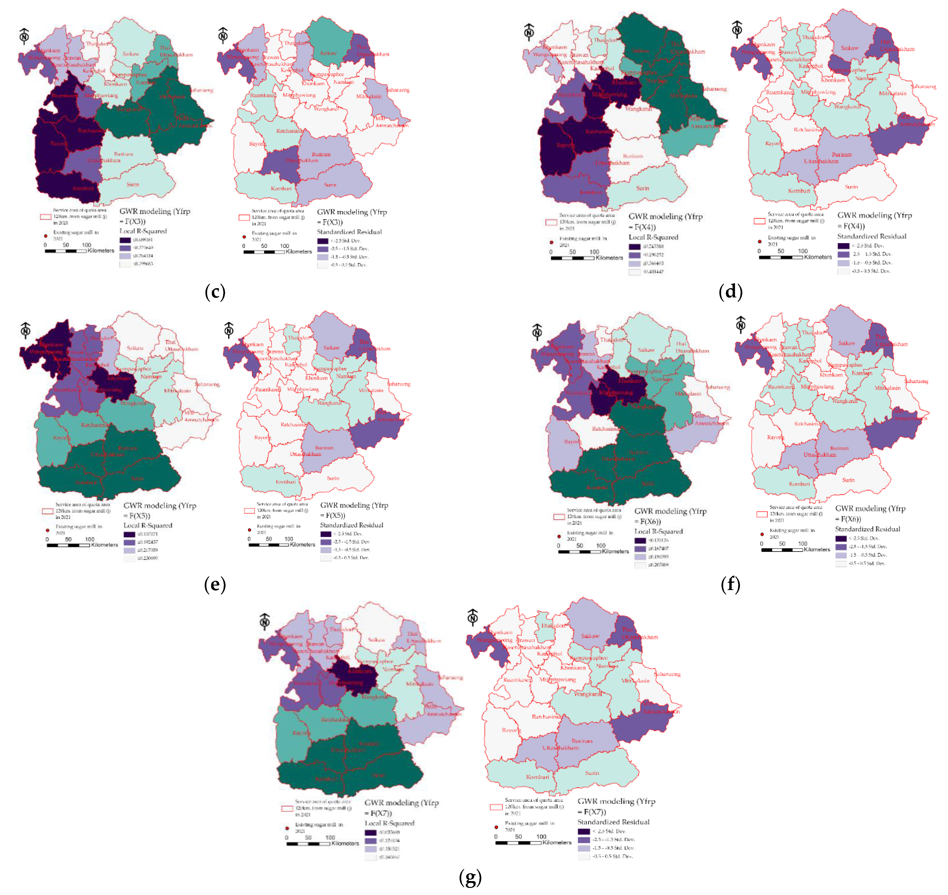
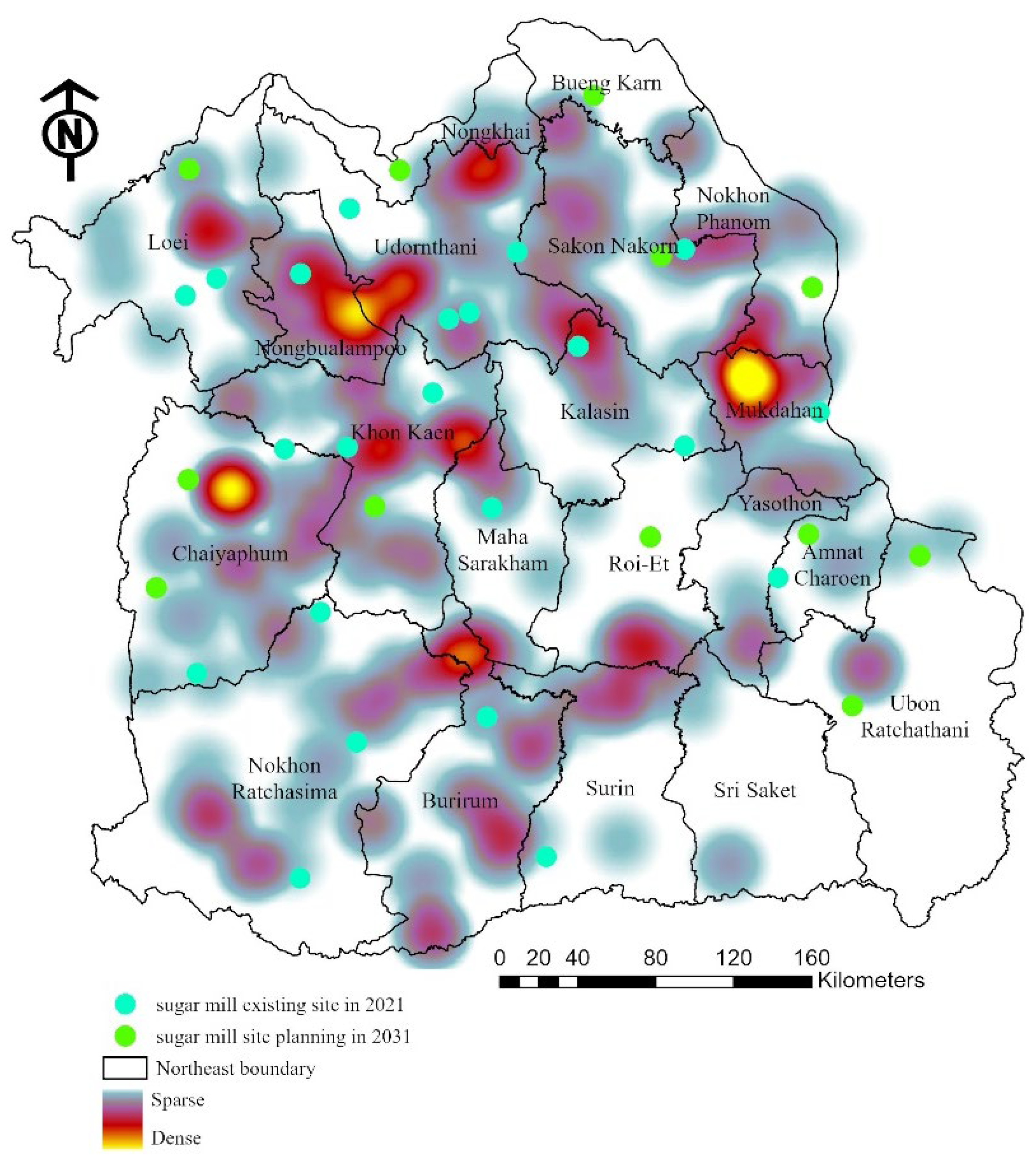
4. Conclusions

The symmetry principle used in the standardization of independent variable data can screen for independent variable factors and enable GWR modeling to actually select a set of variables that are associated with cane burning. The study has confirmed that the GWR model can analyze independent spatial invariables associated with sugarcane burning. When observing local R² and standard residual (SR) index values, the area where the model represents these index values corresponds to the actual data of the OCSB [2]. The hallmark of the GWR model is that the analysis results create relationship models for all spatial units so that they can be used to analyze relationships more flexibly than other models. However, the main principle in using the GWR model to analyze the spatial relationship of cane plot sintering is that there should not be excessively autonomous variables, as this will affect weighted estimates and unnecessary model tolerances from variables that are hypothesized to be associated with cane plot sintering. Selecting a proper factor in the area plays an important role in increasing the accuracy of the model, but in reality, details of the causes of sugarcane burning are rarely given, as this may affect the registration of farmers with sugar mills. The approach to the application of the GWR model in conjunction with the ANN-CA symmetric predictive modeling approach makes it possible to predict the cane burning area in future years with the probability of seeing the trend of area fragmentation, and when comparing the results of the forecast with historical land use data, it can be confirmed that the ANN-CA model, if used with the GWR model, selects factors that correlate to the variables accordingly, increases predictive accuracy. However, the application of the model of a set of independent variables in other areas is essential to know the patterns of sugarcane harvesting of a particular area in order to be able to select the factors that can be applied in all areas, namely distance to transport sugarcane plots index, Percentage of sugarcane plantations in service areas, FRP differences and density of sugarcane yield, and researchers can standardize them with this approach of symmetry.

In future research, real cane plot sintering areas will be examined in some accessible areas in order to analyze the correlation of actual local FRP values to those obtained from satellites and to what level of consistency, as well as a spatial correlation analysis of values. The application guidelines for models in SR low-value service areas will allow them to know the weight value of each factor affecting the acceleration of sugarcane burning, and related agencies such as OCSB will be able to determine the sugarcane harvesting calendar. Designing the sequence of road networks that need to transport sugarcane. Determination of the right of transportation and compensation for agriculture harvested without burning sugarcane in further advanced research, spatial monitoring of cane conversion burning should be increased compared to satellite imagery data, but monitoring the concentration of ${\mathrm{PM}}_{2.5}$ when comparing the percentage of sugarcane plot burning in service zones is also a difficult approach to monitoring.