
Geodesics of a Static Charged Black Hole Spacetime in f(R) Gravity
by
 ,
,
Prateek Sharma
1, 
Hemwati Nandan
1,2,
Gamal G. L. Nashed
2,3,*,
Shobhit Giri
1 and
Amare Abebe
2,4 1
Department of Physics, Gurukula Kangri (Deemed to Be University), Haridwar 249 404, Uttarakhand, India
2
Center for Space Research, North-West University, Mahikeng 2745, South Africa
3
Centre for Theoretical Physics, The British University in Egypt, P.O. Box 43, El Sherouk City 11837, Cairo, Egypt
4
National Institute for Theoretical and Computational Sciences (NITheCS), Mahikeng 2745, South Africa
*
Author to whom correspondence should be addressed.
Symmetry 2022, 14(2), 309; https://doi.org/10.3390/sym14020309
Submission received: 13 November 2021
/
Revised: 12 December 2021
/
Accepted: 15 December 2021
/
Published: 3 February 2022
(This article belongs to the Special Issue Cosmology and Extragalactic Astronomy)
Abstract
:In recent years, the modification of general relativity (GR) through gravity is widely used to study gravity in a variety of scenarios. In this article, we study various physical properties of a black hole (BH) that emerged in the linear Maxwell gravity to constrain the values of different BH parameters, i.e., c and . In particular, we study those values of the defining and c for which the particles around the above-mentioned BH behave like other astrophysical BH in GR. The main motivation of the present research is to study the geodesics equations and discuss the possible orbits for in detail. Furthermore, the frequency shift of a photon emitted by a timelike particle orbiting around the BH is studied given different values of and c. The stability of both timelike and null geodesics is discussed via Lyapunov’s exponent.
1. Introduction
The most tested theory, GR, has proven to be the most successful in the explanation of gravity time and time again. However, one of the significant limitations of GR is that it cannot be renormalized, which further suggests that it cannot be quantized. However, to achieve the renormalization at one loop, the required Einstein–Hilbert action should comprise higher-order curvature terms [1]. Consequently, a modification in the Einstein–Hilbert action is required, so that it comprises higher-order curvature invariants compared to the Ricci scalar [2]. However, these higher-order terms that are required in the action are limited to the strong gravity regimes and, also, are expected to be strongly suppressed by small couplings. The corrections to the GR in this case, therefore, have significance at the Plank scales [3]. Another, more general motivation from cosmology to study the modified theories of gravity is due to the proper explanation of aspects, such as the accelerated expansion of the universe, that cannot be directly interpreted through GR [4]. There is an attempt to explain dark energy, which is believed to be responsible for this accelerated rate of expansion, as some form of modification in GR [5,6,7,8,9,10,11,12,13,14]. To address the issues in GR that arise in high-energy physics to include higher-order invariants into the gravitational action, or from cosmology and astrophysics to obtain a theory more generalized than GR, the gravity is introduced. It is considered to be one of the simplest modifications in GR [3]. The main feature of gravity is that an arbitrary Ricci scalar describes the Lagrangian density. The model that is based on gravity is one of the most elementary theories among several modified theories of gravity used to explain it [15,16,17,18,19,20,21,22,23,24,25,26]. Furthermore, to generalize these theories, another important parameter that should be studied is the impact of electric charge. Therefore, it is necessary to consider electrodynamics field in . The non-linear electrodynamics discussed by Born and Infeld [27] explains very significant aspects, such as the existence of an upper limit on the electric field at the origin of point-like particles. Furthermore, the self-energy is finite for charges [28,29,30]. In this particular study, we have used the linear electrodynamics model.
The observation of the mathematical correspondence between gravitation and electric fields is known since the eighteenth century, where Coulomb built his inverse square law to construct the force between two charges at a radial distance [31]. Therefore, Coulomb’s law is in a complete analog with the gravitational law [32], for which, the force is acting on two masses separated by the same radial distance. The correspondence between this expression of two forces leads scientists to conclude that the gravitational force effected by the sun on the planets could be associated by a magnetic force yielding to the precession of their orbits and, thus, from this point, the gap discovered by Newton in the precession of Mercury’s orbit could be explained. In fact, Mercury’s perihelion precession was exactly explained by Einstein’s GR. Additionally, it is known that gravitation contains a gravitomagnetic field due to the mass current [33,34,35,36]. Moreover, Einstein GR predicts a gravitomagnetic field because of the proper rotation of the Sun that acts on the planetary orbits [37,38,39]. All of the above are known facts that show the importance of the linear, as well as the non-linear, electrodynamics in the frame of Einstein GR and its modifications, including the theory. It is the aim of the present study to study the geodesic of the black hole presented in [40] and to discuss its physics.
The study of null geodesics helps to investigate many physical properties around the BH spacetime, and in particular, the study of the frequency shift can be useful in understanding the strength of a gravitational field around a given spacetime. The investigation for the motion of photons around a Kerr–Sen BH that surfaced from the heterotic string theory has recently been performed through the study of null geodesics (see [41]). The study frequency shift can unveil the gravitational field strength of a distant object and can be very useful in understanding the nature of spacetime around any compact object. A similar type of investigation as in [41] is also performed in [42,43], where the investigation of null geodesics and different types of orbits in the equatorial plane are discussed, along with the study of the frequency shift performed around a magnetically charged BH in dilaton-Maxwell gravity. The method to investigate the properties of these spacetimes are now used to explore the properties of a charged BH in non-linear gravity in the forthcoming sections.
2. Null Geodesics for Static Solution in Non-Linear MAXWELL Gravity
The total action for the static solution of a charged BH in the nonlinear electrodynamics in gravity is given by [44],
where is the determinant of the metric tensor , is the gravitational constant, is the Lagrangian of a non-linear electromagnetic, and in action (1) is the antisymmetric Faraday tensor. In particular, the gauge invariant Lagrangian is written as for the case of linear Maxwell electrodynamics. However, to obtain a corresponding BH spacetime in non-linear Maxwell gravity, an auxiliary field is considered to embed electromagnetism in the framework of GR (In this study, we will consider the linear case of the Maxwell equations of Equation (1) in order to make the discussion of the physics more clear, and will leave the non-linear case of the Maxwell field to a separate case in the near future). For this purpose, we impose the Legendre transformation,
Here, . The auxiliary field, however, is defined as
therefore,
The Lagrangian for the case of this nonlinear electrodynamics model may then be written as [44]
with , here .
The field equations of the action (1) acquire the forms [45,46,47]:
and the corresponding energy-momentum tensor is given as
Using the spherically symmetrical solution corresponding to the action in (1) obtained (with ), the action can be written as [44],
Here, , . The above equation shows that , which ensures that this solution cannot coincide with the BH of GR, which means that it is a novel solution in gravity. The above equation given by Equation (9) is a solution to the class [40] and for the vanishing magnetic field. The parameter c is the one responsible for making the Ricci scalar not vanish. The variation of the event horizon with concerned parameters for the above metric is represented pictorially in Figure 1.
The generalized momenta can be shown as
Here, the dot represents the differentiation with respect to an affine parameter . Furthermore, the Hamiltonian is shown by :
The Hamiltonian is independent of coordinate t and ; further,
The effective potential can be defined as
and from Equations (18) and (19), the effective potential for null geodesics in the case of the above metric can be given by
The nature of the effective potential for the static solution is depicted in Figure 2 which describes the nature of geodesics for particular values of and c. The different values of and the parameter c lie in the range and . It can be easily observed that the value of the effective potential is the same as the BH solution of GR when the value of . Therefore, these values of and c will be considered in order to study the trajectories of photons around this BH solution in this research.
The various types of possible orbits for different values of parameters and c are visually presented in Figure 3; the observations can be useful to constrain the values of and c for astrophysical BHs in GR case. Further, from the trajectories in Figure 3, one can observe that, when the values and are considered, the trajectories obtained are like astrophysical BHs [52].
3. Photon Orbit
The photon orbits define the trajectories of photons around a BH and, to obtain the unstable equation for photon orbits, we solve . Therefore, from (18), the following equations are obtained:
Solving (23), one can obtain the radius of the critical photon orbit as
The critical value of the photon orbit is depicted in Figure 4 and it signifies the radius of the circular orbit around the BH spacetime. It can be easily noticed that the radius decreases as c and increases.
4. The Frequency Shift of Photon Emitted by Timelike Particles
The frequency shift of a photon is an important parameter to determine the degree of curvature in spacetime. The frequency shift of a photon emitted by a timelike particle passing by a BH depends on the BH parameters. If the frequency of an emitted photon shifts toward a smaller value, then it indicates a redshifted photon. The property of the frequency shift can also be useful in evaluating the role of parameters such as and c in more detail. To evaluate the redshift or blueshift emitted by a massive particle orbiting in a circular geodesic around the static BH, one needs to investigate the effective potential for timelike particles [53]. Using Equation (15), with the value of representing the timelike geodesics, Equation (15), along with Equations (16) and (17), can be rewritten as,
The expression for the effective potential for a massive particle, therefore, reads as
For circular orbits, the conditions required are and . Therefore, the expression for constants E and L can be obtained after solving both conditions simultaneously as below:
The expressions for E and L are only valid if and . Further, in order to study the stability of circular geodesics at the equatorial plane, the condition should also be satisfied.
The four-velocity components for the present case can further be defined as:
The angular frequency for the circular geodesic in rgw case of a static solution can be defined as
Therefore, using Equations (31) and (32), it can be further expressed as
Furthermore, the four-momentum for photons is defined as , which follows the null geodesics, i.e., . Therefore, via the Lagrangian, which was defined in (10), the two conserved quantities can be further written as
and
The general expression for the frequency of a photon measured by an observer with at a point in spacetime reads as
where the index c indicates the emission (e) and/or detection (d) at a particular point . Therefore, the frequency of the photon observed by the comoving observer at some emission point (e) can be written as
However, if the observer is far away from the emitter, then the frequency detected is
The four velocities in the four-dimensional spacetime of the emitter orbiting around BH and the distant detector are defined as below:
The four-velocity when the distance between the observer and source is extremely large (i.e., ) can be written as
The frequency shift of the photon emitted by a source moving around BH and detected by a observer can, however, be described as
After, considering the condition that the emitter is in a circular orbit and lies in the equatorial plane (), the red/blueshift can be written as
where is the impact parameter, which can be described by the expression below:
Since there are two different values of D, they correspond to two different values of frequency shifts, which correspond to a photon that is emitted by either a receding object or an approaching object , in the case of a non-rotating BH, . Thus, the redshift is denoted by and the blue-shift is denoted by , which are equal but have opposite signs. The expression for the redshift can be further reduced to the following if the observer is at a very large distance (i.e., ).
Further, the expression for the frequency shift can be obtained as
The frequency shift of the photon emitted by a massive body moving around the BH depends on its parameters. It can easily be observed in Figure 5: as the increases, the value of the redshift decreases with a particular value of the radius () of circular geodesics. Furthermore, the blueshift tends toward a lesser negative value as increases. Further, a similar type of trend can be observed as c increases, where the red frequency shifts toward a lower value for a particular value of and the blue frequency shifts toward the lower negative value for a particular value of .
5. Stability Analysis of Geodesics via Lyapunov Exponents
In this section, we analyze the stability of circular geodesics around the spacetime specified above by calculating Lyapunov exponents, as followed by Cardoso et al. [54]. In general, the Lyapunov exponent is the measure of the average rate of separation between two nearby geodesics in phase space. The positive value of the Lyapunov exponent implies divergence, whereas the negative value implies a convergence of two neighboring geodesics [54,55,56,57,58,59].
The existence of unstable circular geodesics in any gravitational field of BH spacetime consequently verifies the non-linearity of GR and has a positive value of the Lyapunov exponent quantitatively. The non-linearity in GR provides a non-integrability of such a system, due to which, the unstable circular geodesics may show a chaotic nature [60,61,62,63].
Cardoso et al. [54] defined a simple relationship between the second-order derivative of the effective potential and the Lyapunov exponent for the motion of non-spinning test particles in the background of any static, spherically symmetric spacetime as follows:
which are popularly known as the proper time and the coordinate time Lyapunov exponent, respectively. Throughout the calculations, a dot represents a derivative with respect to proper time, and stands for differentiation w.r.t. r.
The circular geodesics are found unstable, stable, and marginally stable for the real, imaginary, and zero value of the Lyapunov exponents, respectively, as shown in Figure 6 [54].
5.1. Stability of Timelike Geodesics
The second-order derivative of effective potential for timelike case from (26) is calculated as
Considering the second order derivative of the effective potential, i.e., from Equation (48) in order to discuss the stability of the circular geodesics of massive particles in non-linear Maxwell gravity, the coordinate time Lyapunov exponent by using Equations (27), (28) and (47) is evaluated as
and the proper time Lyapunov exponent by using Equation (46) is calculated as
The stability or instability of the timelike circular geodesics can be illustrated by Lyapunov exponents calculated above. For , the timelike circular geodesics are stable due to the complex nature (i.e., imaginary) of or . For , the unstable circular geodesics exist due to the real value of or . On the other hand, for , the timelike circular geodesics are marginally stable because both the exponents vanish there. The variation of the coordinate time Lyapunov exponent with a radius of a circular orbit () for various values of parameter c is depicted in Figure 6. It is observed that, for , decreases to a minimum negative value and then increases to zero and becomes constant after a certain value of the radius of circular orbits , but, for other values of c, it exponentially decreases to zero.
The ratio of the proper time Lyapunov exponent () to the coordinate time Lyapunov exponent () is given as
5.2. Stability of Null Geodesics
In the case of massless test particles, only the coordinate time Lyapunov exponent is considered, because there is no proper time for such particles.
The effective potential for massless test particles can again be written as
The null circular orbits are possible when from (18) at constant radius , which provides the angular momentum to energy ratio (i.e., impact parameter), which is given as
The angular frequency at is deduced as
By deriving the second order derivative of with respect to r, i.e., , and using Equation (53), the coordinate time Lyapunov exponent for null circular orbits by using Equation (47) is derived as
The behavior of the Lyapunov exponent () with the radius of null circular orbits () by a varying parameter () is visualized in Figure 7, and we observed that the stability of circular orbits become constant when the radius of circular orbits is larger. The instability of circular orbits near the horizon increases when . However, the instability decreases with an increase in the radius of the circular orbit ( ) and with an increase in the value of for .
The null circular orbits are unstable at the radius , as determined above for real values of the Lyapunov exponent , i.e., for . The instability of unstable null circular orbits can be determined by a quantity known as the instability exponent, which is defined as the ratio of the Lyapunov exponent to the angular frequency (), and is evaluated as follows:
The variation of the instability exponent with respect to radius for the fixed value of parameter is presented in Figure 8. It is clearly observed that the instability of null circular orbits first decreases to a minimum and then increases with .
The variation of the instability exponent with respect to radius is presented in Figure 8. It is found that the instability of null circular orbits first decreases sharply to the minimum and then gradually increases with .
6. Discussion and Conclusions
The study of null geodesics can provide us with information about the structure of spacetime around BHs in the regime of gravity, which is a generalizing modification to GR. This investigation may be further useful for the study of the physical properties of the BHs, given the effect of BH parameters on the trajectories of the photons passing by a BH. The main results drawn from our investigations are as follows.
The variation of the effective potential in the case of the static solution suggests that, when the value of is larger than , the effective potential behaves like the various BH solutions in GR. However, it can be noted that the peak of the effective potential shifted towards lower values as increased. When the effective potential is studied given c, it can be noted that the effective potential also shows a behavior similar to the BH solutions in GR when . Furthermore, the peak of the effective potential increases when c increases within the range of . The possible orbits studied for the BH parameters are set as and ; three types of orbits are observed for different values of impact parameter (b). For , the photon coming from the distant source tends to plunge into the BH. The value of , however, indicates that the photon, when passing the BH, follows a flyby orbit. Further, the photon follows circular geodesics for the value of . The condition for an unstable circular orbit (), in the case of the static solution, is also obtained, and its variation with and c is depicted. It is observed that the value of () decreases with an increase in the value of and value of c.
The study of redshift, which is considered as a direct indicator of gravitational strength, is investigated given different values of BH parameters. The variation of redshift and blueshift is depicted with the radial distance r, which is larger than the radius of the innermost stable circular orbit. It is noticed that, with an increase in , the value of redshift decreases significantly when lies between to . The value of redshift also decreases as c increases when the value of c lies between to .
The stability of timelike and null geodesics is also studied with the help of the Lyapunov exponent with different values of and c. It is observed that the depth of the coordinate time Lyapunov exponent decreases as the value of c increases. Further, an expression for the ratio for the proper time Lyapunov exponent with for timelike geodesics with parameter c is also obtained. The nature of for null geodesics is also studied with , and it is observed that the depth of the instability decreases as increases.
Author Contributions
Conceptualization, P.S., H.N. and G.G.L.N.; formal analysis, S.G. and A.A.; investigation, S.G. and A.A. All authors have read and agreed to the published version of the manuscript.
Funding
This research was funded by Science and Engineering Research Board (SERB), New Delhi through the grant number EMR/2017/000339.
Institutional Review Board Statement
Not applicable.
Informed Consent Statement
Not applicable.
Data Availability Statement
Not applicable.
Acknowledgments
The authors H.N. and P.S. acknowledge the financial support provided by Science and Engineering Research Board (SERB), New Delhi through the grant number EMR/2017/000339. The authors (P.S. and H.N.) also acknowledge the facilities at ICARD, Gurukula Kangri (Deemed to be University), Haridwar, India. The authors also acknowledge that this work is based on the research supported in part by the National Research Foundation (NRF) of South Africa (grant numbers 112131). The authors are also thankful to the anonymous referees for their valuable comments.
Conflicts of Interest
The authors declare no conflict of interest.
References
- Utiyama, R.; DeWitt, B.S. Renormalization of a Classical Gravitational Field Interacting with Quantized Matter Fields. J. Math. Phys. 1962, 3, 608. [Google Scholar] [CrossRef]
- Schmidt, H.-J. Fourth Order Gravity: Equations, History, And Applications to Cosmology. Int. J. Geom. Methods Mod. Phys. 2007, 4, 209. [Google Scholar] [CrossRef]
- Sotiriou, T.P.; Faraoni, V. F(R) Theories of Gravity. Rev. Mod. Phys. 2010, 82, 451. [Google Scholar] [CrossRef] [Green Version]
- Copeland, E.J.; Sami, M.; Tsujikawa, S. Dynamics of Dark Energy. Int. J. Mod. Phys. D 2006, 15, 1753. [Google Scholar] [CrossRef] [Green Version]
- De Felice, A.; Tsujikawa, S. f(R) Theories. Living Rev. Relativ. 2010, 13, 1. [Google Scholar] [CrossRef] [Green Version]
- Kunz, M. The phenomenological approach to modeling the dark energy. C. R. Phys. 2012, 13, 539. [Google Scholar] [CrossRef] [Green Version]
- Nashed, G.G.L. Kerr–Newman Solution and Energy in Teleparallel Equivalent of Einstein Theory. Mod. Phys. Lett. A 2007, 22, 1047. [Google Scholar] [CrossRef] [Green Version]
- Wang, S.; Wang, Y.; Li, M. Holographic dark energy. Phys. Rep. 2017, 696, 1. [Google Scholar] [CrossRef] [Green Version]
- Padmanabhan, T. Dark energy and gravity. Gen. Relativ. Gravit. 2008, 40, 529. [Google Scholar] [CrossRef] [Green Version]
- Sami, M. Models of Dark Energy. In The Invisible Universe: Dark Matter and Dark Energy; Springer: Berlin/Heidelberg, Germany, 2007; pp. 219–256. [Google Scholar]
- Nashed, G.G.L. Brane world black holes in teleparallel theory equivalent to general relativity and their Killing vectors, energy, momentum and angular momentum. Chin. Phys. B 2010, 19, 020401. [Google Scholar] [CrossRef] [Green Version]
- Sahni, V.; Starobinsky, A. Reconstructing Dark Energy. Int. J. Mod. Phys. D 2006, 15, 2105. [Google Scholar] [CrossRef]
- Nashed, G.G.L. Vacuum Nonsingular Black Hole in Tetrad Theory of Gravitation. Nuovo Cim. B 2002, 117, 521. [Google Scholar]
- Nashed, G.G.L. Reissner Nordstrom Solutions and Energy in Teleparallel Theory. Mod. Phys. Lett. 2006, 21, 2241. [Google Scholar] [CrossRef] [Green Version]
- Nojiri, S.; Odintsov, S.D. Unified Cosmic History in Modified Gravity: From F(R) Theory To Lorentz Non-Invariant Models. Phys. Rep. 2011, 505, 59. [Google Scholar] [CrossRef] [Green Version]
- Wheeler, J.T. Symmetric Solutions to the Gauss-Bonnet Extended Einstein Equations. Nucl. Phys. B 1986, 268, 737. [Google Scholar] [CrossRef]
- Nashed, G.; Nojiri, S. Nontrivial Black Hole Solutions in f(R) Gravitational Theory. Phys. Rev. D 2020, 102, 124022. [Google Scholar] [CrossRef]
- Nashed, G.G.L. Rotating Charged Black Hole Spacetimes in Quadratic f(R) Gravitational Theories. Int. J. Mod. Phys. D 2018, 27, 1850074. [Google Scholar] [CrossRef]
- Nashed, G.G.L.; Nojiri, S. Analytic Charged BHs in f(R) Gravity. Phys. Lett. B 2021, 820, 136475. [Google Scholar] [CrossRef]
- Nashed, G.G.L. Spherically symmetric charged black holes in f(R) gravitational theories. Eur. Phys. J. Plus 2018, 133, 18. [Google Scholar] [CrossRef]
- Nashed, G.G.L.; Bamba, K. Charged Spherically Symmetric Taub–NUT Black Hole Solutions in f(R) Gravity. Prog. Theor. Exp. Phys. 2020, 2020, 043E05. [Google Scholar] [CrossRef]
- Antoniadis, I.; Rizos, J.; Tamvakis, K. Singularity-free cosmological solutions of the superstring effective action. Nucl. Phys. B 1994, 415, 497. [Google Scholar] [CrossRef] [Green Version]
- Santos, J.; Alcaniz, J.; Reboucas, M.; Carvalho, F. Energy Conditions in F(R) Gravity. Phys. Rev. D 2007, 76, 083513. [Google Scholar] [CrossRef] [Green Version]
- Nashed, G.G.L. Higher Dimensional Charged Black Hole Solutions in f(R) Gravitational Theories. Adv. High Energy Phys. 2018, 2018, 7323574. [Google Scholar] [CrossRef] [Green Version]
- Nojiri, S.; Odintsov, S.D. Anti-Evaporation of Schwarzschild–De Sitter Black Holes in f(R) Gravity. Class. Quantum Gravity 2013, 30, 125003. [Google Scholar] [CrossRef] [Green Version]
- Shah, P.; Samanta, G.C. Stability Analysis for Cosmological Models in f(R) Gravity Using Dynamical System Analysis. Eur. Phys. J. C 2019, 79, 1. [Google Scholar] [CrossRef]
- Born, M.; Infeld, L. Foundations of the New Field Theory. Proc. Roy. Soc. Lond. A 1934, 144, 425–451. [Google Scholar] [CrossRef]
- Kruglov, S.I. Born-Infeld-Type Electrodynamics and Magnetic Black Holes. Ann. Phys. 2017, 383, 550–559. [Google Scholar] [CrossRef] [Green Version]
- Soleng, H.H. Charged Black Points in General Relativity Coupled to the Logarithmic U(1) Gauge Theory. Phys. Rev. D 1995, 52, 6178–6181. [Google Scholar] [CrossRef] [Green Version]
- Panah, B.E. Can the power Maxwell nonlinear electrodynamics theory remove the singularity of electric field of point-like charges at their locations? Europhys. Lett. 2021, 134, 20005. [Google Scholar] [CrossRef]
- Griffiths, D.J. Introduction to Electrodynamics, 4th ed.; Pearson: Boston, MA, USA, 2013. [Google Scholar]
- Newton, I. Philosophia Naturalis Principia Mathematica; Nabu Press: Charleston, SC, USA, 1687. [Google Scholar]
- Thirring, H. Über die Wirkung rotierender ferner Massen in der Einsteinschen Gravitationstheorie. Phys. Z. 1918, 19, 1–32. [Google Scholar]
- Lense, J.; Thirring, H. Über den Einfluß der Eigenrotation der Zentralkörper auf die Bewegung der Planeten und Monde nach der Einsteinschen Gravitationstheorie. Phys. Z. 1918, 19, 1–14. [Google Scholar]
- Lense, J.; Thirring, H. On the influence of the proper rotation of a central body on the motion of the planets and the moon, according to einstein’s theory of gravitation. Z. Phys. 1918, 19, 156–163. [Google Scholar]
- Ciufolini, I.; Wheeler, J.A. Gravitation and Inertia; Princeton University Press: Princeton, NJ, USA, 1995. [Google Scholar]
- Mashhoon, B.; Hehl, F.W.; Theiss, D.S. On the gravitational effects of rotating masses: The thirring-lense papers. Gen. Relativ. Gravit. 1984, 16, 711–750. [Google Scholar] [CrossRef]
- de Sitter, W. On Einstein’s theory of gravitation and its astronomical consequences. Second paper. Mnras 1916, 77, 155–184. [Google Scholar] [CrossRef] [Green Version]
- Dass, A.; Liberati, S. Gravitoelectromagnetism in metric f(R) and Brans–Dicke theories with a potential. Gen. Rel. Grav. 2019, 51, 84. [Google Scholar] [CrossRef] [Green Version]
- Elizalde, E.; Nashed, G.G.L.; Nojiri, S.; Odintsov, S.D. Spherically Symmetric Black Holes with Electric and Magnetic Charge in Extended Gravity: Physical Properties, Causal Structure, and Stability Analysis in Einstein’s and Jordan’s Frames. Eur. Phys. J. C 2020, 80, 109. [Google Scholar] [CrossRef] [Green Version]
- Uniyal, R.; Nandan, H.; Purohit, K. Null Geodesics and Observables Around the Kerr–Sen Black Hole. Class. Quantum Gravity 2017, 35, 025003. [Google Scholar] [CrossRef] [Green Version]
- Kuniyal, R.S.; Uniyal, R.; Nandan, H.; Purohit, K. Null Geodesics in a Magnetically Charged Stringy Black Hole Spacetime. Gen. Relativ. Gravit. 2016, 48, 46. [Google Scholar] [CrossRef] [Green Version]
- Kuniyal, R.S.; Uniyal, R.; Biswas, A.; Nandan, H.; Purohit, K. Null Geodesics and Red–Blue Shifts of Photons Emitted from Geodesic Particles Around a Noncommutative Black Hole Space–Time. Int. J. Mod. Phys. A 2018, 33, 1850098. [Google Scholar] [CrossRef] [Green Version]
- Nashed, G.; Saridakis, E.N. New Rotating Black Holes in Nonlinear Maxwell F(R) Gravity. Phys. Rev. D 2020, 102, 124072. [Google Scholar] [CrossRef]
- Cognola, G.; Elizalde, E.; Nojiri, S.; Odintsov, S.D.; Zerbini, S. One-loop f(R) gravity in de Sitter Universe. J. Cosmol. Astropart. Phys. 2005, 2, 010. [Google Scholar] [CrossRef] [Green Version]
- Ayon-Beato, E.; Garcia, A. New Regular Black Hole Solution from Nonlinear Electrodynamics. Phys. Lett. B 1999, 464, 25. [Google Scholar] [CrossRef] [Green Version]
- Koivisto, T.; Kurki-Suonio, H. Cosmological Perturbations in the Palatini Formulation of Modified Gravity. Class. Quant. Grav. 2006, 23, 2355. [Google Scholar] [CrossRef]
- Hod, S. Spherical Null Geodesics of Rotating Kerr Black Holes. Phys. Lett. B 2013, 718, 1552. [Google Scholar] [CrossRef] [Green Version]
- Uniyal, R.; Nandan, H.; Jetzer, P. Bending Angle of Light in Equatorial Plane of Kerr–Sen Black Hole. Phys. Lett. B 2018, 782, 185. [Google Scholar] [CrossRef]
- Sharma, P.; Nandan, H.; Gannouji, R.; Uniyal, R.; Abebe, A. Deflection of Light by a Rotating Black Hole Surrounded by “Quintessence”. Int. J. Mod. Phys. A 2020, 35, 2050155. [Google Scholar] [CrossRef]
- Kala, S.; Nandan, H.; Sharma, P. Deflection of Light around a Rotating BTZ Black Hole. Mod. Phys. Lett. A 2020, 35, 2050323. [Google Scholar] [CrossRef]
- Nashed, G. Uniqueness of Non-Trivial Spherically Symmetric Black Hole Solution in Special Classes of F(R) Gravitational Theory. Phys. Lett. B 2021, 812, 136012. [Google Scholar] [CrossRef]
- Becerril, R.; Valdez-Alvarado, S.; Nucamendi, U. Obtaining Mass Parameters of Compact Objects from Redshifts and Blueshifts Emitted by Geodesic Particles around Them. Phys. Rev. D 2016, 94, 124024. [Google Scholar] [CrossRef] [Green Version]
- Cardoso, V.; Miranda, A.S.; Berti, E.; Witek, H.; Zanchin, V.T. Geodesic stability, Lyapunov exponents, and quasinormal modes. Phys. Rev. D 2009, 79, 064016. [Google Scholar] [CrossRef] [Green Version]
- Giri, S.; Nandan, H. Stability Analysis of Geodesics and Quasinormal Modes of a Dual Stringy Black Hole via Lyapunov Exponents. Gen. Relativ. Gravit. 2021, 53, 1. [Google Scholar] [CrossRef]
- Sano, M.; Sawada, Y. Measurement of the Lyapunov Spectrum from a Chaotic Time Series. Phys. Rev. Lett. 1985, 55, 1082. [Google Scholar] [CrossRef] [PubMed]
- Pradhan, P. Stability Analysis and Quasinormal Modes of Reissner–Nordstrom Space-Time via Lyapunov Exponent. Pramana 2016, 87, 5. [Google Scholar] [CrossRef] [Green Version]
- Mondal, M.; Pradhan, P.; Rahaman, F.; Karar, I. Geodesic Stability and Quasi Normal Modes Via Lyapunov Exponent for Hayward Black Hole. Mod. Phys. Lett. A 2020, 35, 2050249. [Google Scholar] [CrossRef]
- Pradhan, P. The Thirteenth Marcel Grossmann Meeting: On Recent Developments in Theoretical and Experimental General Relativity, Astrophysics and Relativistic Field Theories; World Scientific: Stockholm, Sweden, 2015; pp. 1892–1894. [Google Scholar]
- Cornish, N.J.; Levin, J. Lyapunov timescales and black hole binaries. Class. Quantum Gravity 2003, 20, 1649. [Google Scholar] [CrossRef] [Green Version]
- Cornish, N.J. Chaos and gravitational waves. Phys. Rev. D 2001, 64, 084011. [Google Scholar] [CrossRef] [Green Version]
- Hilborn, R.C. Chaos and Nonlinear Dynamics: An Introduction for Scientists and Engineers; Oxford University Press on Demand: Oxford, UK, 2000. [Google Scholar]
- Suzuki, S.; Maeda, K.-I. Chaos In Schwarzschild Spacetime: The Motion of a Spinning Particle. Phys. Rev. D 1997, 55, 4848. [Google Scholar] [CrossRef] [Green Version]
Figure 1.
Variation of event horizon for different values with for different values of c; here, dashed line represents the negative root and solid line represents the positive root.
Figure 1.
Variation of event horizon for different values with for different values of c; here, dashed line represents the negative root and solid line represents the positive root.
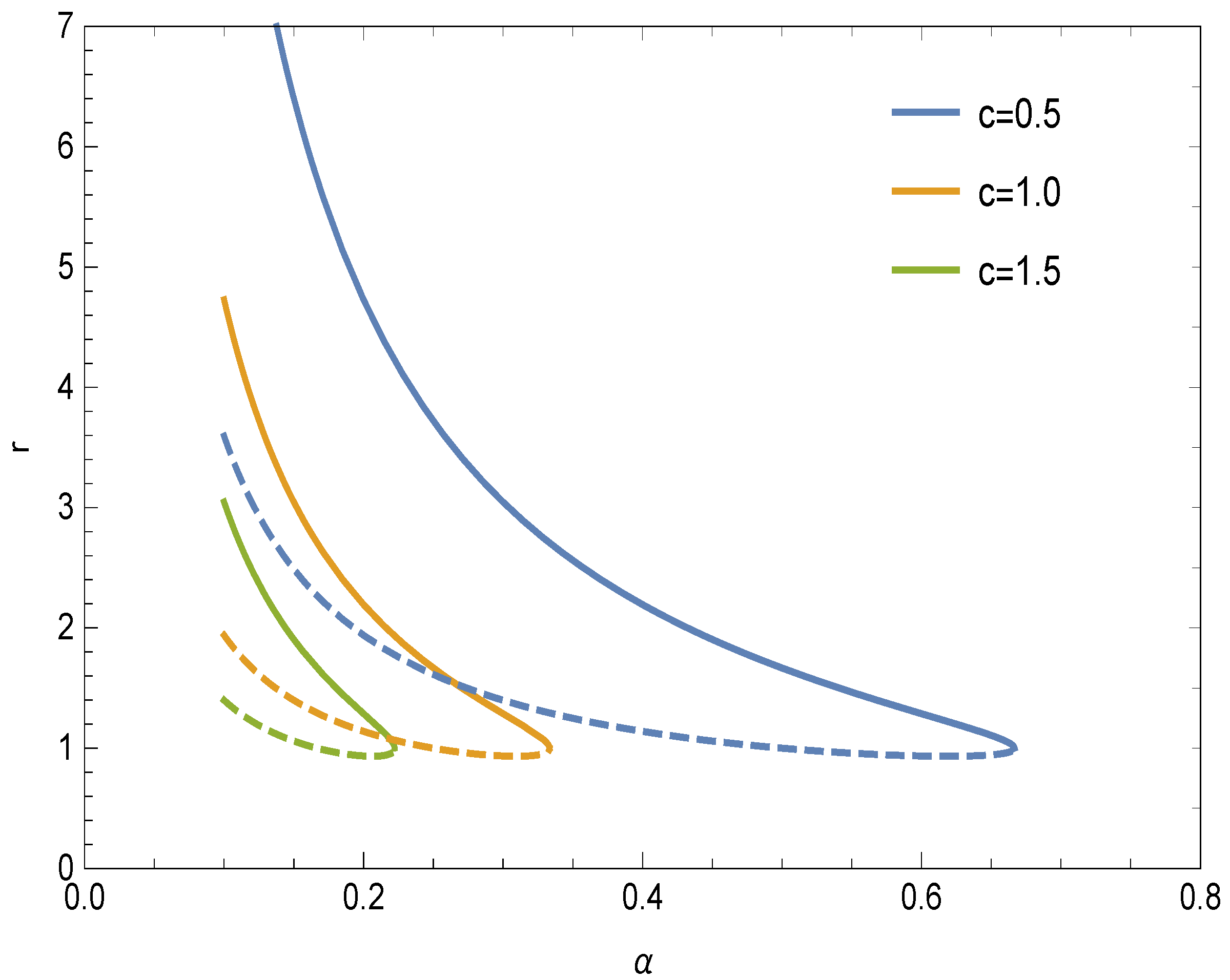
Figure 2.
Effective potential for various values of (i) ((a) panel) and (ii) c ((b) panel).
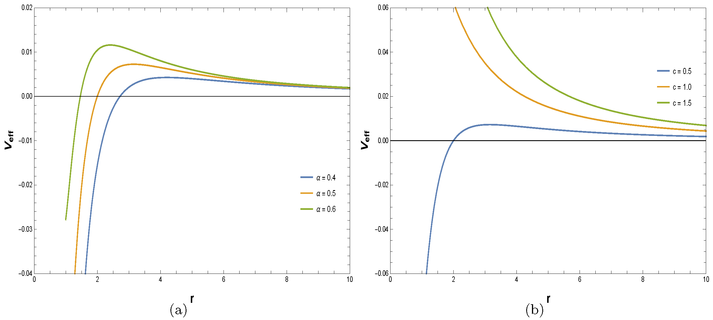
Figure 3.
The trajectory of photon and shape of effective potential for and , (a,b) (top) panel—plunge orbit at , (ii) (c,d) (middle) panel—flyby orbit with (e,f) (iii) (bottom) panel—circular orbit with .
Figure 3.
The trajectory of photon and shape of effective potential for and , (a,b) (top) panel—plunge orbit at , (ii) (c,d) (middle) panel—flyby orbit with (e,f) (iii) (bottom) panel—circular orbit with .
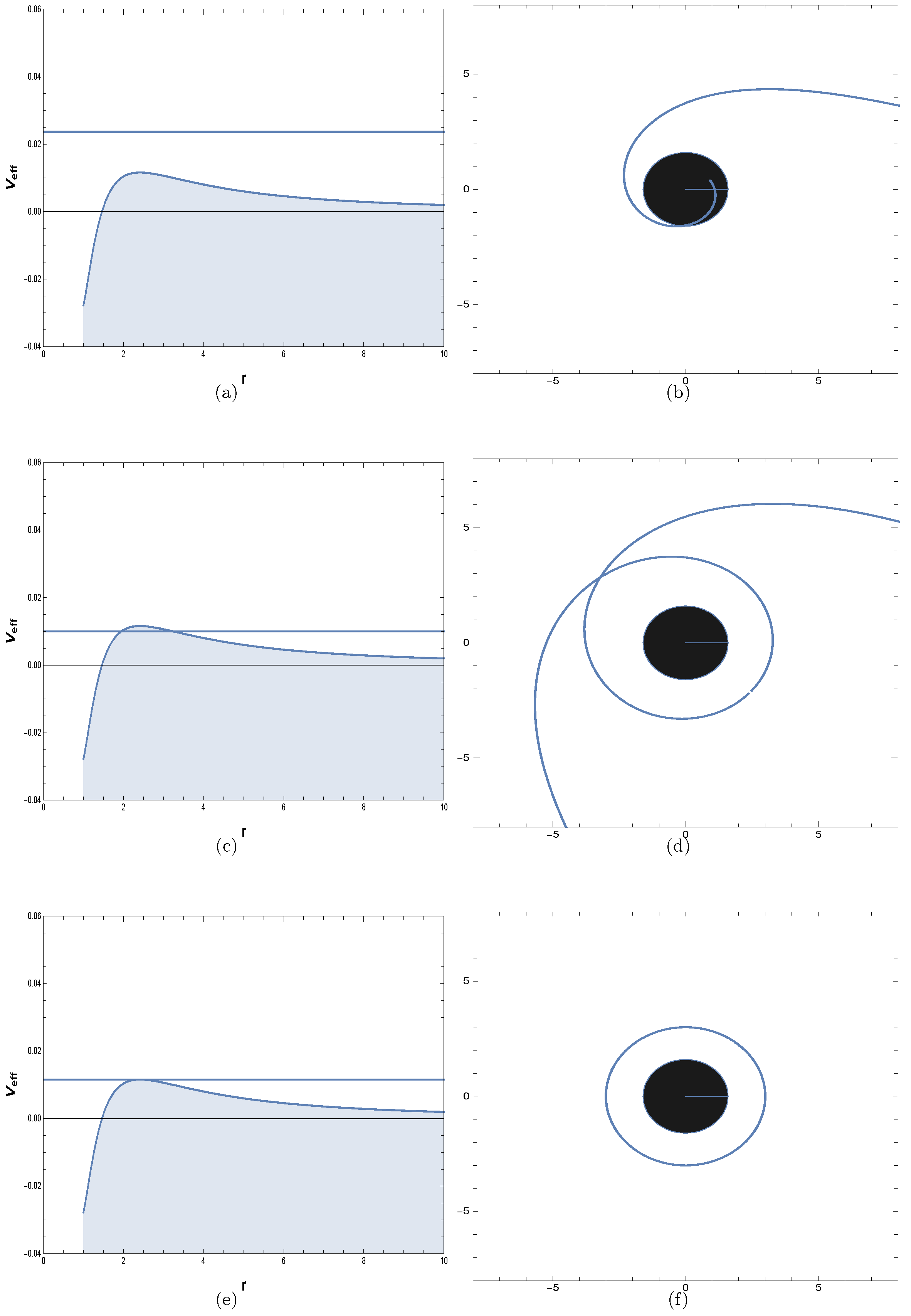
Figure 4.
The variation of radius of critical photon orbit with (a) for different values of c and with (b) c for different values of .
Figure 4.
The variation of radius of critical photon orbit with (a) for different values of c and with (b) c for different values of .
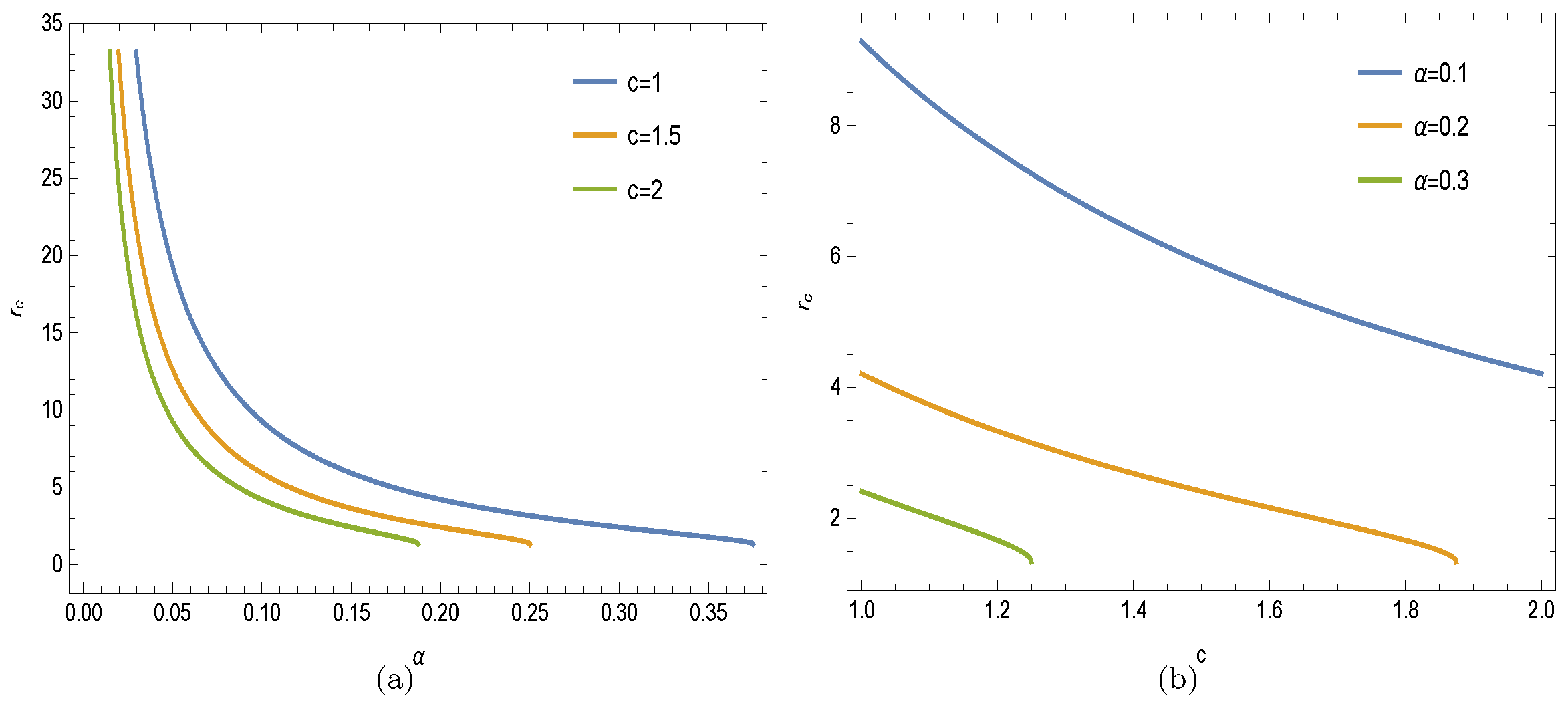
Figure 5.
The variation of redshift ((left) panel) and blueshift ((right) panel) for different values of (a) (upper panel) and (b) c (lower panel).
Figure 5.
The variation of redshift ((left) panel) and blueshift ((right) panel) for different values of (a) (upper panel) and (b) c (lower panel).

Figure 6.
The variation of “” for “” for a massive test particle with different values of c and for the fixed value of .
Figure 6.
The variation of “” for “” for a massive test particle with different values of c and for the fixed value of .
Figure 7.
The behavior of “” with radius “” for massless particles with different values of parameter and fixed value of .
Figure 7.
The behavior of “” with radius “” for massless particles with different values of parameter and fixed value of .

Figure 8.
The variation of “” with radius “” for massless particles with parameter and fixed value of .
Figure 8.
The variation of “” with radius “” for massless particles with parameter and fixed value of .
Publisher’s Note: MDPI stays neutral with regard to jurisdictional claims in published maps and institutional affiliations. |
© 2022 by the authors. Licensee MDPI, Basel, Switzerland. This article is an open access article distributed under the terms and conditions of the Creative Commons Attribution (CC BY) license (https://creativecommons.org/licenses/by/4.0/).
Share and Cite
MDPI and ACS Style
Sharma, P.; Nandan, H.; Nashed, G.G.L.; Giri, S.; Abebe, A. Geodesics of a Static Charged Black Hole Spacetime in f(R) Gravity. Symmetry 2022, 14, 309. https://doi.org/10.3390/sym14020309
AMA Style
Sharma P, Nandan H, Nashed GGL, Giri S, Abebe A. Geodesics of a Static Charged Black Hole Spacetime in f(R) Gravity. Symmetry. 2022; 14(2):309. https://doi.org/10.3390/sym14020309
Chicago/Turabian StyleSharma, Prateek, Hemwati Nandan, Gamal G. L. Nashed, Shobhit Giri, and Amare Abebe. 2022. "Geodesics of a Static Charged Black Hole Spacetime in f(R) Gravity" Symmetry 14, no. 2: 309. https://doi.org/10.3390/sym14020309
Note that from the first issue of 2016, this journal uses article numbers instead of page numbers. See further details here.