
Anisotropic Compact Stars in D → 4 Limit of Gauss–Bonnet Gravity

1
Centre for Theoretical Physics, The British University in Egypt, P.O. Box 43, Cairo 11837, Egypt
2
Laboratory for Theoretical Cosmology, Tomsk State University of Control Systems and Radioelectronics (TUSUR), 634050 Tomsk, Russia
3
Institut de Ciències de l’Espai (ICE-CSIC/IEEC), Campus, c. Can Magrans s/n, 08193 Barcelona, Spain
4
Institució Catalana de Recerca i Estudis Avançats (ICREA), 08010 Barcelona, Spain
5
Department of Physics, Aristotle University of Thessaloniki, 54124 Thessaloniki, Greece
*
Author to whom correspondence should be addressed.
Symmetry 2022, 14(3), 545; https://doi.org/10.3390/sym14030545
Submission received: 2 February 2022
/
Revised: 28 February 2022
/
Accepted: 1 March 2022
/
Published: 7 March 2022
(This article belongs to the Special Issue Cosmology and Extragalactic Astronomy)
Abstract
:In the frame of Gauss–Bonnet gravity and in the limit of , based on the fact that spherically symmetric solution derived using any of regularization schemes will be the same form as the original theory, we derive a new interior spherically symmetric solution assuming specific forms of the metric potentials that have two constants. Using the junction condition we determine these two constants. By using the data of the star EXO 1785-248, whose mass is and radius km, we calculate the numerical values of these constants, in terms of the dimensionful coupling parameter of the Gauss–Bonnet term, and eventually, we get real values for these constants. In this regard, we show that the components of the energy–momentum tensor have a finite value at the center of the star as well as a smaller value to the surface of the star. Moreover, we show that the equations of the state behave in a non-linear way due to the impact of the Gauss–Bonnet term. Using the Tolman–Oppenheimer–Volkoff equation, the adiabatic index, and stability in the static state we show that the model under consideration is always stable. Finally, the solution of this study is matched with observational data of other pulsars showing satisfactory results.
1. Introduction
To date, a considerable amount of observational data of compact stellar objects data, such as neutron stars and spherically symmetric black holes are available from gravitational-wave (GW) detectors, like X-ray observations, advanced LIGO [1], Kagra [2,3], advanced Virgo [4], and from the networks of radio telescopes, like the event horizon telescope [5], from the NICER mission [6] and there is much activity in the study of such objects as well, i.e., neutron stars in [7,8]. In the frame of current observational uncertainties, all data are consistent with Einstein’s general relativity (GR) and despite this. However, there is a venue for a extended gravity theories, which might be useful to future observations that require alternative descriptions than that of Einstein’s GR theory, like, for example, the curious GW190814 event [9]. Regardless of the direct tests of Einstein GR, there are also pending questions to be clarified, like the maximum mass of neutron stars, the high-density equation of state (EoS), and so on. The observations obtained recently by the compact object merger GW190814 [9] shows that the low-mass component of the binary possesses a mass of , which directly puts it in the present observational mass gap between neutron stars and black holes. Moreover, among the gravitational waves, there are three events/candidates involving the merger of one neutron star or light mass black hole with another compact object. If this event is described solely by GR, the lower mass component of the binary can either be a neutron star with an unexpectedly stiff (or exotic) EoS, a black hole with an unexpectedly small mass, or a neutron star with an unexpectedly rapid rotation [10,11,12,13,14,15,16,17,18,19,20,21,22,23,24,25,26,27,28,29,30,30]. On the other hand, an natural and non-exotic description of the lower mass component of the event GW190814 can be given by extended gravity [31,32,33]. In the frame of modified gravitational theories there are many studies tackling the problem of anisotropic compact stars for example in the frame of , where R is the Ricci scalar and G is the Gauss–Bonnet term [34], in the frame of mimetic theory [35], in the frame of [36,37,38,39], in the frame of teleparallel gravity [40,41], and in the frame of scalar Gauss–Bonnet theory [42].
To date, two GW outcomes have been verified as binary neutron star (BNS) mergers, GW170817 [43] and GW190425 [44], and extra outcomes are anticipated in the near future [45]. Revealing of the GW from the inspiral phase of GW170817, in connection with observations of its kilonova electromagnetic counterpart [46,47,48], have put new constraints on the dimensionless tidal deformability of neutron stars and hence on their EoS [49,50,51,52,53,54,55,55]. Such EoS constraints are expected to be more precise in the next years, via the combination of a larger number of observations [56,57,58,59,60]. Despite the sensitivity of the advanced LIGO and advanced Virgo detectors, these were not sensitive enough in order to determine the post-merger phase in GW170817 [43,61]. However, this post-merger phase may be revealed in the near future, by several experiments and collaborations, like [45], or by third-generation detectors [62,63], or even with high-frequency detectors [64,65]. The observation of GW in the post-merger phase of a BNS merger would then offer another opportunity to probe the high-density EoS of NSs, see [66,67,68,69,70,71,72,73,74,75,76,77].
In view of the future observational data which might indicate deviations from GR, it is important to study compact objects in the context of extended theories of gravity. In the present work, we will study compact objects in the context of Einstein–Gauss–Bonnet gravity (EGB) [78,79] which provides a number of attractive analytic solutions. The action of this theory is given as:
with , and is the Gauss–Bonnet scalar while is the matter Lagrangian. Here has a dimension of length squared. We will then formulate models of neutron stars, and by using numerical methods we will study several solutions for neutron stars.
Lately, Glavan and Lin [80] provided a new general covariant modified model of the EGB theory that elucidates multiple non-trivial issues taking place in 4-dimensional spacetime. Note that such scenario to get consistent 2-dimensional GR from D-dimensional GR in the limit of was proposed in [81,82]. The GB expression () in 4-dimensions is a total derivative term and hence does not impact the gravitational dynamics. However, on a higher dimension, i.e., , it involves an exterior result of the total derivative. When , Torii et al. [83] and Mardones et al. [84] showed that the support of the GB term is proportional to a vanishing factor in 4-dimensions. Moreover, Glavan and Lin [80] rescaled the dimensional parameter , i.e., showing behavior very much identical to GR behavior, as it preserves equal degrees of freedom in all dimensions and sets aside the Ostrogradsky instability [85]. Using the regularization of the GB expression at , one can derive a non-trivial impact in the four-dimensional dynamics [86,87,88,89,90].
Here, we stress the fact that the novel 4D EGB theory [80] has got several quibbles. The criticisms on the correctness by taking the limit have been discussed in [91,92]. Nevertheless, it was shown in References [93,94,95] that in 4-dimensions spacetime the output field equations are not regular and no regular action which creates the proposed regularized field equations can be exist [96]. The Kaluza–Klein reduction method of the limit yields a special class of scalar-tensor theories in the Horndeski family [97,98]. Similar method was used in [88,99,100] by adding a counter term in D-dimensions and then taking limit. Furthermore, many projects have been analyzed the previous issues coming from the new 4-dimensions EGB gravity. Depending on the selection of the regularization method, several theories have been presented with various degrees of freedom and various characteristic. Using the procedure of [90,91], the handling was shown to be symmetrical by ignoring the 4-dimensions diffeomorphism invariance. Nevertheless, it is interesting to note that spherically symmetric 4-dimensions solutions are valid in these regularized theories [87]. Actually, black hole solutions through the rescaling method [80] still correct in these regularized theories [88,89]. Therefore, it becomes clear that the spherically symmetric solution derived using any of these regularization schemes will be identical to the authentic theory. In this frame, the interior spherically symmetric star solution is significant to study. Therefore, we decide to obtain the field equations starting with outlines depending on the new 4-dimensions EGB gravity. Moreover, one of the motivations of the present study is to constrain the numerical value of Gauss–Bonnet parameter in the frame of the anisotropic model so that we get a realizable astrophysical model. Additionally, we want to test the behavior of the equation of state in this model and compared it with Einstein general relativity.
The GB theory has various applications in different topics of gravity and, therefore, it appeared to be quite unconventional to scientists in the field of cosmology and astrophysics. Glavan and Lin [80] in the frame of GB theory derived a static spherically symmetric vacuum black hole which was proved to be quite different from Schwarzschild black holes. Gurses et al. [95] showed that EGB theory does not support any intrinsic 4-dimensional solution in terms of the metric, thus its viability of the black hole solutions is appropriate for the case . More applications of EGB theory were used to calculate the thermodynamics of non-rotating and rotating black holes and evaluate the thermodynamical quantities such as entropy, mass, and temperature [101,102,103,104]. Moreover, EGB theory is used for the study of various black hole related issues, like thermodynamics of AdS black holes [105], quasi-normal modes [106], black gravitational lensing of strong and weak types [101], Hawking radiation [107], geodesic motions for spinning test particles [108], and wormhole solutions [109]. Aside from the issues of the black hole, EGB theory is applied for the study of neutron stars, which is a subject of continuous research interest. Recent observations of neutron stars have further constrained the equation of state of nuclear matter, but the inner structure of neutron stars still remains a mystery. An investigation of the photon sphere and the shadow observed by a distant observer and the exploration of the effects of black hole parameters have been studied in the frame of EGB [110].
The determination of the inner core matter is quite non-trivial as the composition varies with the nature of interaction and quark matter, hyperon matter, Bose–Einstein condensate, strange mesons are all considered to be the core matter. However, the invention of 2 neutron stars like PSR J1614-2230 [] [10] and J0348+0432 [] [111] brought criterion on the nature of the core matter. Quantum chromodynamics (QCD), supports the conversion of hadronic matter into deconfined quarks inside the neutron stars. This invention makes the Bodmer–Witten hypothesis quite important to the context as it already predicted for a quark-matter component in the cosmic rays detected from neutron stars [112,113]. This strengthens the presence of quark stars.
The present study aims to derive interior solutions for EGB theory, using the fact that spherically symmetric solution obtained from any regularization methods will be identical with the original theory [87,88,89], and then check the physical viability of such a solution. According to the procedure, it is possible to construct self-consistent compact stellar models capable of describing anisotropic neutron stars in the context of EGB gravity. The layout of the present paper is as follows: In Section 2, a summary of EGB theory is reported. Additionally, in Section 2, we apply the field equation of EGB to D-dimensional spherically symmetric spacetime and write them in the limit and solve the resulting differential equations assuming specific forms of the metric potentials. In Section 3, we use the junction condition, i.e. match the interior solution with the exterior solution derived [80], and fix the two constants that characterize our solution. In Section 4, we discuss the physical conditions that any real compact star must satisfy and show that the energy components of our model have finite values at the center of the star and decrease towards the star of the surface. Moreover, we show that the model under consideration has a positive anisotropy which means that the tangential pressure is greater than the radial one. Additionally, we prove that our model satisfies the causality condition and the energy–momentum conditions. Finally, we study the equation of state, (EoS), and show that the impact of Gauss–Bonnet expression makes its pattern has a non-linear form. In Section 5, we show that our model is stable under various conditions, like the TOV equation, adiabatic index, and the static state. We confront our results with observational data and summarizing the output results in Section 5. Finally, the conclusions follow in the end of the paper (in this study, we are going to use the geometrized units).
2. Compact Star in Gauss–Bonnet Theory
The Lagrangian of Einstein–Gauss–Bonnet, in D—dimensional spacetime has the form:
whose corresponding action takes the form:
where is the Ricci scalar curvature and is the Gauss–Bonnet invariant associated with the D-dimensional spacetime. The dimensionful parameter is the Gauss–Bonnet coupling parameter and is the action contributed from the matter perfect fluid. The Gauss–Bonnet term, , takes the form:
where and are the Ricci curvature and Riemann curvature tensors, respectively. Variation of the action (3) with respect to the metric tensor yields:
where the Einstein tensor , the Lancoz tensor and the stress tensor are defined respectively as:
The field Equation (5) has no meaning when . In spite of this, Glavan et al. [80,114] show that using a re-scale of the parameter as and by specifying spacetimes of curvature scale which are maximally symmetric that set the variation of GB contribution as:
that shows in a clear way the non-vanishing of when .
Now we consider a spacetime of D—dimensions that has the form:
where, refers to the -dimensional surface of a unit sphere.
As shown in [80], the effective 4-dimensional theory is obtained in the singular limit with . Using the limit we derive the dimensionally reduced field equations as:
where the “prime” indicates differentiation with respect to the radial coordinate.
Moreover, we suppose that the stress energy–momentum tensor of anisotropic fluid has the form:
where is the energy density, and are the radial and tangential pressures, where is the time-like vector defined as and is the unit radial vector with its spacelike property, defined by such that and . In the present study, we shall consider the matter content described by the energy density , radial and tangential pressures, and respectively (throughout this study we shall use geometrized units in which ).
The above system of differential Equations (11)–(13), constitutes three differential equations with five variables, thus we need two extra conditions. In this study we are going to assume the metric potentials and to have special forms so that the resulting model can be consistent with a real compact star. Here we assume
where and are constants that will be fixed from the junction conditions. We assume the ansatz given by Equation (15) so that we can get non-singular values of energy density, and radial and tangential pressures and also finite values of these quantities at the center of the star as we will show in the following sections. Using Equation (15) in Equations (11)–(13) we get the form of energy density, radial and tangential pressures which are quite lengthy to quote them here and therefore, we present these in Appendix A. In the next section we are going to fix the two constants using the junction conditions, i.e., we will match the interior solution with an exact exterior solution.
3. Junction Conditions
The vacuum spherically symmetric solution in Gauss–Bonnet gravitational theory is derived in [80] and has the following form in the limit :
where the unknown function has the form
In this study, we consider the negative branch in Equation (17) that yields (The matching condition of the positive branch of Equation (17) yields unphysical quantities, that is, negative values of density, radial and tangential pressures. So we will not consider this case in this study):
Equation (18) shows that the direct effect of the GB parameter will be of order and in case we neglect it we will return to the usual Schwarzschild solution. Now matching the interior and exterior spacetimes at the boundary , i.e., yields the value of the two constants and which are:
where . Now we are going to calculate the derivative of the metric potentials (15) and the exterior solution given by Equation (18) and get:
The second junction condition should be checked as well which deals with the first derivative of the metric with respect to the radial coordinate. Having the results in Equation (21), one can check the second junction condition to see whether it trivially satisfies or one needs to consider a shell with an appropriate energy–momentum tensor.
4. Physics of the Solution
Now, we are ready to examine if the interior solution which is given in Appendix A can describe a realistic star. For such a purpose, we are going to derive some necessary conditions which must be satisfied in order to have a real star.
4.1. Energy–Momentum Tensor
For any real interior solution, we must have a positive value of all the components of the energy–momentum tensor, i.e., the energy density, and the radial and transverse pressures should have positive well-defined values. Additionally, all these components must be finite at the center of the star and should decrease in the radial direction towards the surface of the star. Finally, the tangential pressure should exceed the radial one at the center of the star. In the present study we shall consider the stellar model of the observed pulsar EXO 1785-248 whose mass is and its radius km for which the constants and can be calculated numerically. We must stress that the model solution given in Appendix A cannot be reduced to the GR solution because the parameter is not allowed to take zero values. We depict the components of energy–momentum in Figure 1. The numerical values of the parameters and used in Figure 1 are . Moreover, , , and . Figure 1 ensures that the energy density, and radial and tangential pressures are decreasing towards the surface stellar. Additionally, in Figure 1d, we present the behavior of the anisotropy parameter which is defined as . Moreover, in Figure 1d we present the anisotropic force that has a positive behavior which means that we have a repulsive force, due to the fact .
4.2. Causality
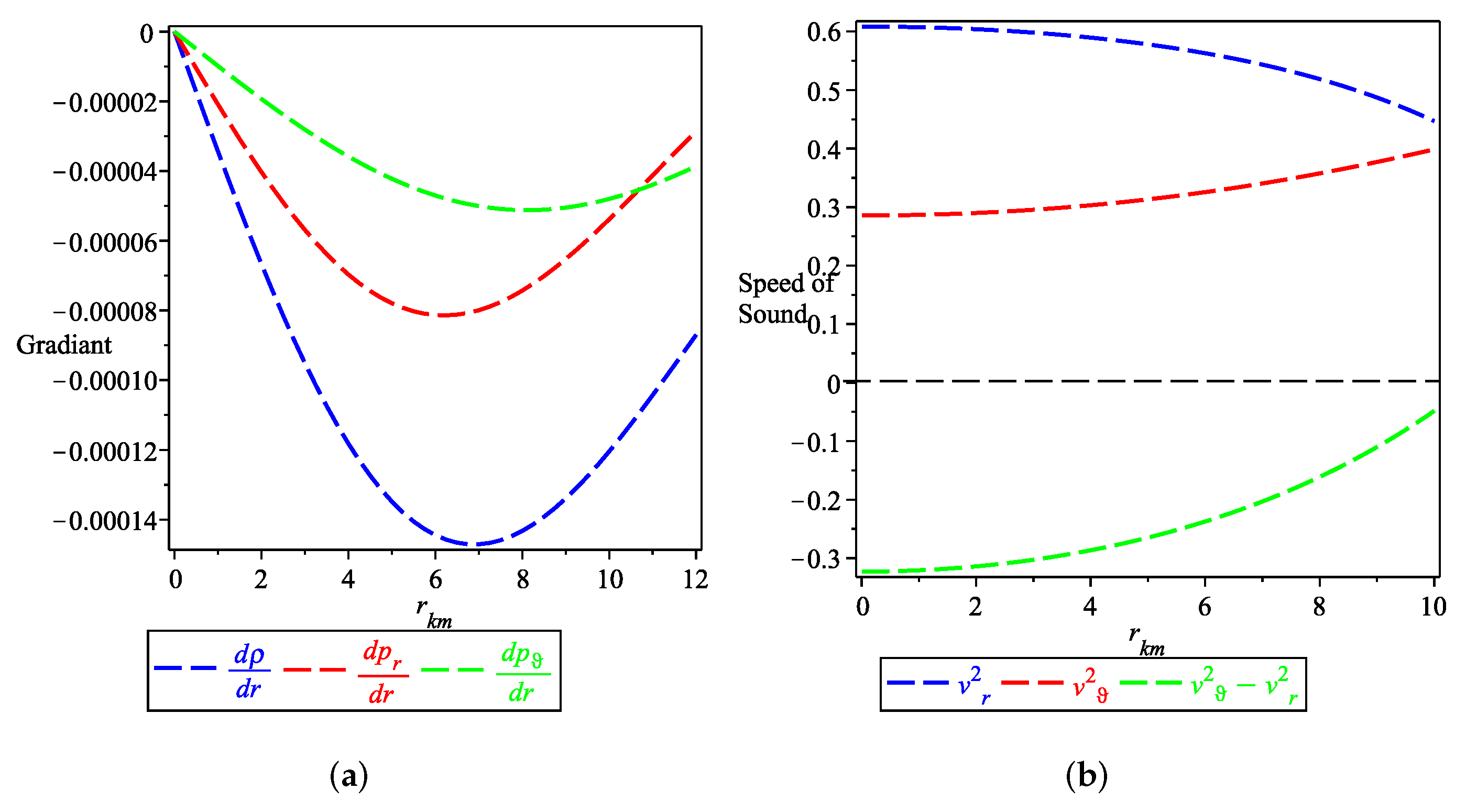
To test the behavior of the sound velocities, we evaluate the derivative of the energy–density and the radial and tangential pressures, the final expressions of which we present in Appendix B. The equations given in Appendix B do not inform us if the gradients of the components of the energy–momentum tensor have a positive or negative behavior, therefore, we plot them in Figure 2a and from the plots it is ensured that the gradients of the energy–momentum tensor are negative, as it is required for any realistic physical stellar.
To verify the causality conditions we must prove that the radial and transverse sound speeds, and , have values less than the speed of light. We evaluate these quantities, and , and we present their functional forms in Appendix C. We plot the equations given in Appendix C in Figure 2b to ensure the validity of the conditions and .
The appearance of non-vanishing radial force with different signs in different regions of the fluid is called gravitational cracking. This happens when the radial force is directed inwards in the inner part of the sphere for all values of the radial coordinate r between the center, and some value beyond which the force reverses its direction [115]. It is shown in Reference [116] that a simple requirement to avoid gravitational cracking is . In Figure 2b, we show that the solution given in Appendix C is stable against cracking.
4.3. Energy Conditions
Energy conditions are considered as important tests for non-vacuum solutions. To satisfy the dominant energy condition (DEC), we have to prove that & . As shown in Figure 3a the DEC is satisfied for suitable choices of the parameters , , and . Additionally, in Figure 3b–d we show that the weak energy condition (WEC), the null energy condition (NEC), and the strong energy condition (SEC) are all satisfied. It is interesting to note that the problem of energy conditions in the frame of has been studied and the results presented in this study are consistent with the results presented in [117].
4.4. Mass–Radius Relation
The compactification factor, , is the one defined as the ratio between the mass and radius. It has an important role towards to revealing the physical properties of compact objects. Starting from the solution given in Appendix A, we define the gravitational mass by the following expression:
where we substitute the value of energy density from the first equation presented in Appendix A. The compactification factor is then defined as:
Substituting Equation (22) into (23), one can get the explicit form of the compactification factor. The behavior of the gravitational mass and the compactification factor are plotted in Figure 4 which indicates in a clear way that the gravitational mass and the compactification factor are directly proportional to the radial coordinate.
4.5. Equation of State
Finally, let us study the equation of state (EoS) of a compact stellar object as presented in [118] which uses a linear EoS. In the present case, we show that the EoS is not linear due to the contribution of the GB term. To show this, we define the radial and transverse EoS as:
with and being the radial and transverse EoS parameters. Using the form of energy density and radial, and tangential pressures presented in Appendix A we get the EoSs of our model as presented in Appendix D. As it can be seen in Figure 4b, the EoS is non-linear because of the contribution of the GB term.
Now, we are going to calculate the EoS as , for such purpose we write . Using the form of energy density given in Appendix A we get the form of the radial, tangential and pressure components in Appendix D. The behavior of the EoS as a function of the energy density is presented in Figure 4c–e. As it can be seen in Figure 4c–e, the radial and tangential EoS parameters are positive, while the total EoS, i.e., is negative.
5. Stability of the Model
We use two different procedures to study the stability problem, the first is the Tolman–Oppenheimer–Volkoff (TOV) equation and the second is to study the adiabatic index. Now we are going to discuss the TOV equation in the frame of our solution is presented in Appendix A.
5.1. The Tolman–Oppenheimer–Volkoff Equation
To study the stability of our solution displayed in Appendix A, we are going to suppose the hydrostatic equilibrium by using the TOV equation [119,120] as given in [121]:
Here represents the gravitational mass evaluated at the radius r and has the following form:
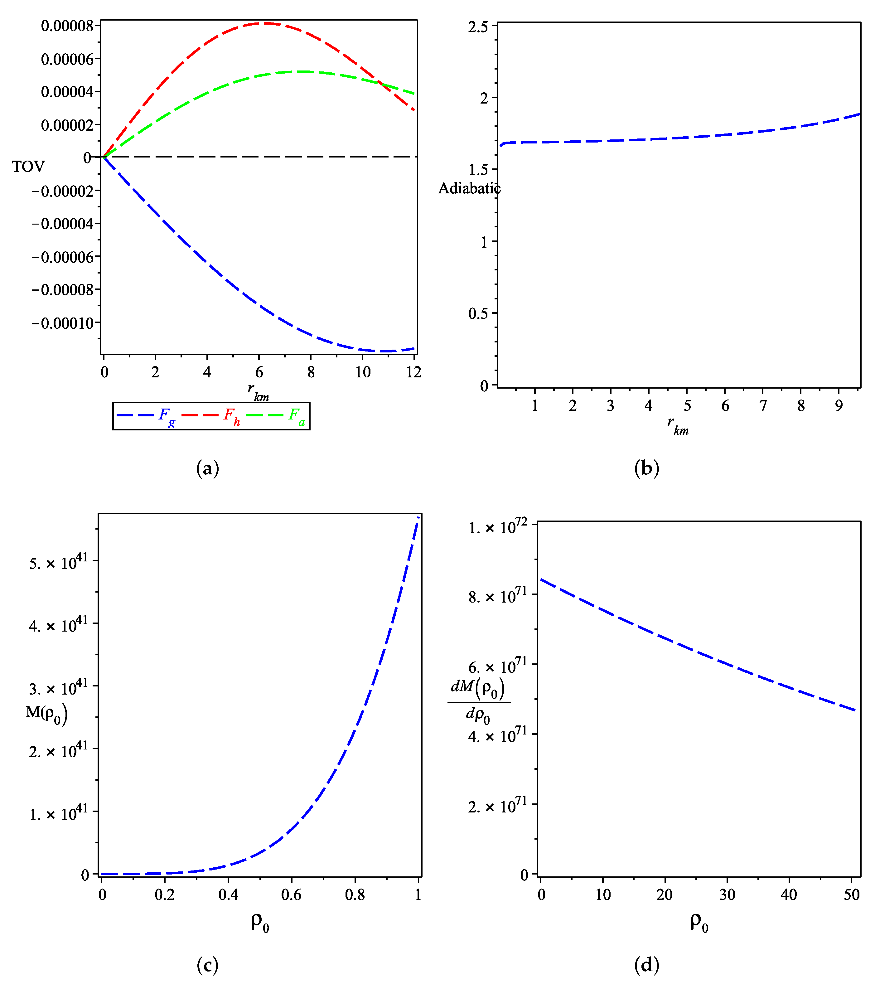
Here , , and are the gravitational mass, the anisotropic, and the hydrostatic forces, respectively. The explicit forms of these forces can be found in Appendix E. We plot the different forces presented in Appendix E in Figure 5a, and it can be seen, it is ensured that the hydrostatic and anisotropic forces are positive and dominate over the gravitational force, which has a negative value, hence opposite direction, and the system is kept in static equilibrium.
5.2. The Adiabatic Index
The adiabatic index connects the structure of a spherically symmetric static object to the EoS of the interior solution. One can use the adiabatic index to discuss the stability of the interior solution [122]. For any interior solution, it becomes stable if its adiabatic index is greater than [123] however, if , then the isotropic sphere is in neutral equilibrium. Following Chan et al. [124], the stability condition of a relativistic anisotropic sphere, , must be satisfied. Here is defined as
where the collapse happens according to the nature of the anisotropy. When one can have and the system still stable and when one can have unstable system even if . The behavior of the adiabatic index is shown in Figure 5b which ensures the stability condition of our solution.
5.3. Stability in the Static State
Finally, let us study the stability through the procedure given by Harrison, Zeldovich, and Novikov [125,126,127] who showed that for stable compact stars the mass, (which is a function of the central density) must be positive and increasing and also the derivative of the mass with respect to the central density must have a positive value, i.e., . Applying this condition to our model we get the density at the center of the star:
Using Equation (29) in Equation (22) we get the form of mass in terms of the central density which is written in Appendix F. The pattern of the derivative of mass with respect to the central density given by the equation presented in Appendix and it is plotted in Figure 5d which ensures the stability of our model.
6. Discussion and Conclusions
Among the higher curvature theories, the EGB theory offers new possibilities for gravity. This new proposal has received much interest because the GB invariant may share Einstein’s field equations through the redefinition of the GB constant to be in D-dimensions and taking the limit . Inspired by this new proposal of EGB theory, in this work, we rigorously explained a static and spherically symmetric interior solution. Assuming a specific form of the metric potentials, we derived in this new proposal of EGB a new interior solution. In this study we showed that the GB parameter, , must take a tiny negative value otherwise we will have imaginary quantities for the components of pressures. As we showed the effect of the constant acting on the EoS, yielded its behavior to behave in a non-linear form, unlike Einstein GR.
We checked the impact of the anisotropy regime and showed that it is always positive which means that we have a repulsive force. Moreover, we listed the physical conditions that any real star must satisfy and showed that our model yields:
- i
- A well-known behavior of the energy density and radial and tangential pressures at the center as well as at the surface of the star as shown in Figure 1a–c.
- ii
- iii
- In Figure 3 we showed that the energy conditions which must be satisfied for any realistic star are satisfied.
- iv
- Using different techniques, TOV, adiabatic index, and stability of the static state, we studied the stability of our model and we showed that it is stable as Figure 5a,b,d show. The results of this study can be applied to the observational data of various stars showing consistent results as shown in Table 1 and Table 2. For these objects, it is possible to calculate the density at the center and at the surface, the radial and tangential speed, at the center and the surface of the star, the SEC at the center and the surface of the star, and the redshift at the surface of the star. It is interesting to see that all the results of the different stars of our solution are compatible with observations. From the above discussions we can say that our results presented in this study are in agreement with that presented in [129] from the viewpoint of the structure of compact star.
In summary, we derived a new interior solution in the framework of EGB in the limit , assuming physically motivated metric potentials. This solution has a non-trivial form of the Ricci scalar as well as the GB term. The internal solution can be matched with the external in the limit . In a forthcoming paper, we will consider a similar situation assuming a charged interior solution.
Author Contributions
Conceptualization, G.G.L.N.; Supervision, S.D.O.; Writing—review and editing, V.K.O. All authors have read and agreed to the published version of the manuscript.
Funding
This research received no external funding.
Institutional Review Board Statement
Not applicable.
Informed Consent Statement
Not applicable.
Data Availability Statement
Not applicable.
Acknowledgments
The authors would like to thank the referees for their valuable comments. This work was supported by MINECO (Spain), project PID2019-104397GB-I00 and Unidad de Excelencia MarAa de Maeztu CEX2020-001058-M( SDO).
Conflicts of Interest
The authors declare no conflict of interest.
Appendix A. Energy Density and Radial and Tangential Pressures
Now, let us present the quantities related to the interior solution discussed in the present study and write them as:
where is the anisotropy defined as .
Appendix B. The Gradients of Energy Density and Radial and Transverse Pressures
The gradients of the components of the energy–momentum tensor given in the Appendix A take the following form:
where , and .
Appendix C. Derivation of the Radial and Tangential Speeds of Sound
Using the equations of the gradient of energy–momentum components presented in Appendix B we get:
Appendix D. Derivation of the EoS’s
Using the form of energy density and radial and tangential pressures presented in Appendix A, we get the EoS as:
Using the approximate form of the energy density listed in Appendix A we get:
where the first equation of Equation (A5) has four roots and we write only the real one given by the second equation of Equation (A5). The second equation of (A5) ensures that the constant must not equal zero and . Using Equation (A5) in the form of and displayed in Appendix A we get:
where ,
=, .
Appendix E. The Different Forces on the Model
Appendix F. The Form of the Mass in Terms of the Central Density at the Surface of the Star
The form of the mass in terms of the central density at the surface of the star takes the form:
. The form of the derivative of w.r.t. the central density takes the form
References
- The LIGO Scientific Collaboration; Aasi, J.; Abbott, B.P.; Abbott, R.; Abbott, T.; Abernathy, M.R.; Ackley, K.; Adams, C.; Adams, T.; Addesso, P.; et al. Advanced ligo. Class. Quantum Gravity 2015, 32, 074001. [Google Scholar]
- Somiya, K. Detector configuration of KAGRA–the Japanese cryogenic gravitational-wave detector. Class. Quantum Gravity 2012, 29, 124007. [Google Scholar] [CrossRef] [Green Version]
- Aso, Y.; Michimura, Y.; Somiya, K.; Ando, M.; Miyakawa, O.; Sekiguchi, T.; Tatsumi, D.; Yamamoto, H. Interferometer design of the KAGRA gravitational wave detector. Phys. Rev. D 2013, 88, 043007. [Google Scholar] [CrossRef] [Green Version]
- Acernese, F.; Agathos, M.; Agatsuma, K.; Aisa, D.; Allemandou, N.; Allocca, A.; Amarni, J.; Astone, P.; Balestri, G.; Ballardin, G.; et al. Advanced Virgo: A second-generation interferometric gravitational wave detector. Class. Quantum Gravity 2014, 32, 024001. [Google Scholar] [CrossRef] [Green Version]
- Psaltis, D. Event Horizon Telescope. Phys. Rev. Lett. 2020, 125, 141104. [Google Scholar] [CrossRef] [PubMed]
- Raaijmakers, G.; Greif, S.K.; Riley, T.E.; Hinderer, T.; Hebeler, K.; Schwenk, A.; Watts, A.L.; Nissanke, S.; Guillot, S.; Lattimer, J.M.; et al. Constraining the dense matter equation of state with joint analysis of NICER and LIGO/Virgo measurements. Astrophys. J. Lett. 2020, 893, L21. [Google Scholar] [CrossRef]
- Astashenok, A.V.; Capozziello, S.; Odintsov, S.D. Further stable neutron star models from f (R) gravity. J. Cosmol. Astropart. Phys. 2013, 12, 040. [Google Scholar] [CrossRef] [Green Version]
- Astashenok, A.V.; Capozziello, S.; Odintsov, S.D. Maximal neutron star mass and the resolution of the hyperon puzzle in modified gravity. Phys. Rev. D 2014, 89, 103509. [Google Scholar] [CrossRef] [Green Version]
- Abbott, R.; Abbott, T.D.; Abraham, S.; Acernese, F.; Ackley, K.; Adams, C.; Adhikari, R.X.; Adya, V.B.; Affeldt, C.; Agathos, M.; et al. GW190814: Gravitational waves from the coalescence of a 23 solar mass black hole with a 2.6 solar mass compact object. Astrophys. J. Lett. 2020, 896, L44. [Google Scholar] [CrossRef]
- Huang, K.; Hu, J.; Zhang, Y.; Shen, H. The possibility of the secondary object in GW190814 as a neutron star. Astrophys. J. 2020, 904, 39. [Google Scholar] [CrossRef]
- Bombaci, I.; Drago, A.; Logoteta, D.; Pagliara, G.; Vidaña, I. Was GW190814 a black hole–Strange quark star system? Phys. Rev. Lett. 2021, 126, 162702. [Google Scholar] [CrossRef] [PubMed]
- Roupas, Z.; Panotopoulos, G.; Lopes, I. QCD color superconductivity in compact stars: Color-flavor locked quark star candidate for the gravitational-wave signal GW190814. Phys. Rev. D 2021, 103, 083015. [Google Scholar] [CrossRef]
- Zhou, X.; Li, A.; Li, B.-A. R-mode Stability of GW190814’s Secondary Component as a Supermassive and Superfast Pulsar. Astrophys. J. 2021, 910, 62. [Google Scholar] [CrossRef]
- Awad, A.; Nashed, G. Generalized teleparallel cosmology and initial singularity crossing. J. Cosmol. Astropart. Phys. 2017, 2017, 046. [Google Scholar] [CrossRef]
- Most, E.R.; Papenfort, L.J.; Weih, L.R.; Rezzolla, L. A lower bound on the maximum mass if the secondary in GW190814 was once a rapidly spinning neutron star. Mon. Not. R. Astron. Soc. Lett. 2020, 499, L82. [Google Scholar] [CrossRef]
- Nashed, G.G.L. Schwarzschild solution in extended teleparallel gravity. EPL Europhys. Lett. 2014, 105, 10001. [Google Scholar] [CrossRef] [Green Version]
- Nashed, G.G.L. Charged Axially Symmetric Solution, Energy and Angular Momentum in Tetrad Theory of Gravitation. Int. J. Mod. Phys. A 2006, 21, 3181. [Google Scholar] [CrossRef] [Green Version]
- Tan, H.; Noronha-Hostler, J.; Yunes, N. Neutron Star Equation of State in light of GW190814. Phys. Rev. Lett. 2020, 125, 261104. [Google Scholar] [CrossRef]
- Vattis, K.; Goldstein, I.S.; Koushiappas, S.M. Could the 2.6 M⊙ object in GW190814 be a primordial black hole? Phys. Rev. D 2020, 102, 061301. [Google Scholar] [CrossRef]
- Zhang, N.B.; Li, B.A. GW190814’s Secondary Component with Mass 2.50–2.67 M⊙ as a Superfast Pulsar. Astrophys. J. 2020, 902, 38. [Google Scholar] [CrossRef]
- Fattoyev, F.J.; Horowitz, C.J.; Piekarewicz, J.; Reed, B. GW190814: Impact of a 2.6 solar mass neutron star on nucleonic equations of state. Phys. Rev. C 2020, 102, 065805. [Google Scholar] [CrossRef]
- Shirafuji, T.; Nashed, G.G.L.; Kobayashi, Y. Equivalence principle in the new general relativity. Prog. Theor. Phys. 1996, 96, 933. [Google Scholar] [CrossRef] [Green Version]
- Tsokaros, A.; Ruiz, M.; Shapiro, S.L. GW190814: Spin and equation of state of a neutron star companion. Astrophys. J. 2020, 905, 48. [Google Scholar] [CrossRef]
- Tews, I.; Pang, P.T.; Dietrich, T.; Coughlin, M.W.; Antier, S.; Bulla, M.; Heinzel, J.; Issa, L. On the nature of GW190814 and its impact on the understanding of supranuclear matter. Astrophys. J. Lett. 2021, 908, L1. [Google Scholar] [CrossRef]
- Dexheimer, V.; Gomes, R.O.; Klähn, T.; Han, S.; Salinas, M. GW190814 as a massive rapidly-rotating neutron star with exotic degrees of freedom. Phys. Rev. C 2021, 103, 025808. [Google Scholar] [CrossRef]
- Godzieba, D.A.; Radice, D.; Bernuzzi, S. On the maximum mass of neutron stars and GW190814. Astrophys. J. 2021, 908, 122. [Google Scholar] [CrossRef]
- Kanakis-Pegios, A.; Koliogiannis, P.S.; Moustakidis, C.C. Probing the Nuclear Equation of State from the Existence of a ~2.6 M⊙ Neutron Star: The GW190814 Puzzle. Symmetry 2021, 13, 183. [Google Scholar] [CrossRef]
- Nathanail, A.; Most, E.R.; Rezzolla, L. GW170817 and GW190814: Tension on the maximum mass. Astrophys. J. Lett. 2021, 908, L28. [Google Scholar] [CrossRef]
- Roupas, Z. Secondary component of gravitational-wave signal GW190814 as an anisotropic neutron star. Astrophys. Space Sci. 2021, 366, 9. [Google Scholar] [CrossRef]
- Biswas, B.; Nandi, R.; Char, P.; Bose, S.; Stergioulas, N. GW190814: On the properties of the secondary component of the binary. Mon. Not. R. Astron. Soc. 2021, 505, 1600–1606. [Google Scholar] [CrossRef]
- Nunes, R.C.; Coelho, J.G.; de Araujo, J.C. Weighing massive neutron star with screening gravity: A look on PSR J0740+6620 and GW190814 secondary component. Eur. Phys. J. C 2020, 80, 1115. [Google Scholar] [CrossRef]
- Astashenok, A.V.; Capozziello, S.; Odintsov, S.D.; Oikonomou, V.K. Extended gravity description for the GW190814 supermassive neutron star. Phys. Lett. B 2020, 811, 135910. [Google Scholar] [CrossRef]
- Astashenok, A.V.; Capozziello, S.; Odintsov, S.D.; Oikonomou, V.K. Causal limit of neutron star maximum mass in f (R) gravity in view of GW190814. Phys. Lett. B 2020, 816, 136222. [Google Scholar] [CrossRef]
- Mustafa, G.; Shamir, M.F.; Tie-Cheng, X. Physically viable solutions of anisotropic spheres in f(R,G) gravity satisfying the Karmarkar condition. Phys. Lett. B 2020, 101, 104013. [Google Scholar] [CrossRef]
- Nashed, G.G.L. Anisotropic compact stars in the mimetic gravitational theory. Astrophys. J. 2021, 919, 113. [Google Scholar] [CrossRef]
- Nashed, G.G.L.; Odintsov, S.D.; Oikonomou, V.K. Anisotropic compact stars in higher-order curvature theory. Eur. Phys. J. C 2021, 81, 528. [Google Scholar] [CrossRef]
- Nashed, G.G.L.; Capozziello, S. Anisotropic compact stars in f (R) gravity. Eur. Phys. J. C 2021, 81, 481. [Google Scholar] [CrossRef]
- Astashenok, A.V.; Capozziello, S.; Odintsov, S.D.; Oikonomou, V.K. Maximum Baryon Masses for Static Neutron Stars in f(R) Gravity. Europhys. Lett. 2021. [Google Scholar] [CrossRef]
- Astashenok, A.V.; Capozziello, S.; Odintsov, S.D.; Oikonomou, V.K. Novel stellar astrophysics from extended gravity. EPL Europhys. Lett. 2021, 134, 59001. [Google Scholar] [CrossRef]
- Nashed, G.G.L.; Abebe, A.; Bamba, K. Neutral physical compact spherically symmetric stars with non-exotic matters in Einstein’s cluster model using Weitzenböck. Eur. Phys. J. C 2020, 80, 1109. [Google Scholar] [CrossRef]
- Nashed, G.G.L.; Capozziello, S. Stable and self-consistent compact star models in teleparallel gravity. Eur. Phys. J. C 2020, 80, 969. [Google Scholar] [CrossRef]
- Övgün, A. Black hole with confining electric potential in scalar-tensor description of regularized 4-dimensional Einstein-Gauss-Bonnet gravity. Phys. Lett. B 2021, 820, 136517. [Google Scholar] [CrossRef]
- Abbott, B.P.; Abbott, R.; Abbott, T.D.; Acernese, F.; Ackley, K.; Adams, C.; Adams, T.; Addesso, P.; Adhikari, R.X.; Adya, V.B. GW170817: Observation of gravitational waves from a binary neutron star inspiral. Phys. Rev. Lett. 2017, 119, 161101. [Google Scholar] [CrossRef] [PubMed] [Green Version]
- Abbott, B.P.; Abbott, R.; Abbott, T.D.; Abraham, S.; Acernese, F.; Ackley, K.; Adams, C.; Adhikari, R.X.; Adya, V.B.; Affeldt, C. GW190425: Observation of a compact binary coalescence with total mass 3.4 M⊙. Astrophys. J. Lett. 2020, 892, L3. [Google Scholar] [CrossRef]
- Abbott, B.P.; Abbott, R.; Abbott, T.D.; Abraham, S.; Acernese, F.; Ackley, K.; Adams, C.; Adya, V.B.; Affeldt, C.; Agathos, M. Prospects for observing and localizing gravitational-wave transients with Advanced LIGO, Advanced Virgo and KAGRA. Living Rev. Rel. 2018, 23, 3. [Google Scholar] [CrossRef] [PubMed]
- Abbott, B.P.; Bloemen, S.; Canizares, P.; Falcke, H.; Fender, R.P.; Ghosh, S.; Groot, P.; Hinderer, T.; Hörandel, J.R.; Jonker, P.G. Multi-messenger observations of a binary neutron star merger. Astrophys. J. Lett. 2017, 848, L12. [Google Scholar] [CrossRef]
- Abbott, B.P.; Abbott, R.; Abbott, T.D.; Acernese, F.; Ackley, K.; Adams, C.; Adams, T.; Addesso, P.; Adhikari, R.X.; Adya, V.B. Gravitational Waves and Gamma-rays from a Binary Neutron Star Merger: GW170817 and GRB 170817A. Astrophys. J. Lett. 2017, 848, L13. [Google Scholar] [CrossRef]
- Goldstein, A.; Veres, P.; Burns, E.; Briggs, M.S.; Hamburg, R.; Kocevski, D.; Wilson-Hodge, C.A.; Preece, R.D.; Poolakkil, S.; Roberts, O.J. An Ordinary Short Gamma-Ray Burst with Extraordinary Implications: Fermi-GBM Detection of GRB 170817A. Astrophys. J. Lett. 2017, 848, L14. [Google Scholar] [CrossRef] [Green Version]
- Bauswein, A.; Just, O.; Janka, H.T.; Stergioulas, N. Neutron-star radius constraints from GW170817 and future detections. Astrophys. J. Lett. 2017, 850, L34. [Google Scholar] [CrossRef] [Green Version]
- Abbott, B.P.; Abbott, R.; Abbott, T.D.; Acernese, F.; Ackley, K.; Adams, C.; Adams, T.; Addesso, P.; Adhikari, R.X.; Adya, V.B. GW170817: Measurements of Neutron Star Radii and Equation of State. Phys. Rev. Lett. 2018, 121, 161101. [Google Scholar] [CrossRef] [Green Version]
- Capano, C.D.; Tews, I.; Brown, S.M.; Margalit, B.; De, S.; Kumar, S.; Brown, D.A.; Krishnan, B.; Reddy, S. Stringent constraints on neutron-star radii from multimessenger observations and nuclear theory. Nat. Astron. 2020, 4, 625–632. [Google Scholar] [CrossRef]
- Thapa, V.B.; Kumar, A.; Sinha, M. Baryonic dense matter in view of gravitational-wave observations. Mon. Not. R. Astron. Soc. 2021, 507, 2991–3004. [Google Scholar] [CrossRef]
- Dietrich, T.; Coughlin, M.W.; Pang, P.T.; Bulla, M.; Heinzel, J.; Issa, L.; Tews, I.; Antier, S. Multimessenger constraints on the neutron-star equation of state and the Hubble constant. Science 2020, 370, 1450–1453. [Google Scholar] [CrossRef] [PubMed]
- Breschi, M.; Perego, A.; Bernuzzi, S.; Del Pozzo, W.; Nedora, V.; Radice, D.; Vescovi, D. AT2017gfo: Bayesian inference and model selection of multicomponent kilonovae and constraints on the neutron star equation of state. Mon. Not. R. Astron. Soc. 2021, 505, 1661–1677. [Google Scholar] [CrossRef]
- Chatziioannou, K. Neutron-star tidal deformability and equation-of-state constraints. Gen. Rel. Grav. 2020, 52, 109. [Google Scholar] [CrossRef]
- Del Pozzo, W.; Li, T.G.; Agathos, M.; Van Den Broeck, C.; Vitale, S. Demonstrating the feasibility of probing the neutron-star equation of state with second-generation gravitational-wave detectors. Phys. Rev. Lett. 2013, 111, 071101. [Google Scholar] [CrossRef]
- Chatziioannou, K.; Yagi, K.; Klein, A.; Cornish, N.; Yunes, N. Probing the Internal Composition of Neutron Stars with Gravitational Waves. Phys. Rev. D 2015, 92, 104008. [Google Scholar] [CrossRef] [Green Version]
- Lackey, B.D.; Wade, L. Reconstructing the neutron-star equation of state with gravitational-wave detectors from a realistic population of inspiralling binary neutron stars. Phys. Rev. D 2015, 91, 043002. [Google Scholar] [CrossRef] [Green Version]
- Vivanco, F.H.; Smith, R.; Thrane, E.; Lasky, P.D.; Talbot, C.; Raymond, V. Measuring the neutron star equation of state with gravitational waves: The first forty binary neutron star merger observations. Phys. Rev. D 2019, 100, 103009. [Google Scholar] [CrossRef] [Green Version]
- Chatziioannou, K.; Han, S. Studying strong phase transitions in neutron stars with gravitational waves. Phys. Rev. D 2020, 101, 044019. [Google Scholar] [CrossRef] [Green Version]
- Abbott, B.P.; Abbott, R.; Abbott, T.D.; Acernese, F.; Ackley, K.; Adams, C.; Adams, T.; Addesso, P.; Adhikari, R.X.; Adya, V.B. Search for post-merger gravitational waves from the remnant of the binary neutron star merger GW170817. Astrophys. J. Lett. 2017, 851, L16. [Google Scholar] [CrossRef]
- Abbott, B.P.; Abbott, R.; Abbott, T.D.; Abernathy, M.R.; Ackley, K.; Adams, C.; Addesso, P.; Adhikari, R.X.; Adya, V.B.; Affeldt, C. Exploring the sensitivity of next generation gravitational wave detectors. Class. Quantum Gravity 2017, 34, 044001. [Google Scholar] [CrossRef] [Green Version]
- Maggiore, M.; Van Den Broeck, C.; Bartolo, N.; Belgacem, E.; Bertacca, D.; Bizouard, M.A.; Branchesi, M.; Clesse, S.; Foffa, S.; Garcia-Bellido, J.; et al. Science case for the Einstein telescope. J. Cosmol. Astropart. Phys. 2020, 3, 050. [Google Scholar] [CrossRef] [Green Version]
- Ganapathy, D.; McCuller, L.; Rollins, J.G.; Hall, E.D.; Barsotti, L.; Evans, M. Tuning Advanced LIGO to kilohertz signals from neutron-star collisions. Phys. Rev. D 2021, 103, 022002. [Google Scholar] [CrossRef]
- Page, M.A.; Goryachev, M.; Miao, H.; Chen, Y.; Ma, Y.; Mason, D.; Rossi, M.; Blair, C.D.; Ju, L.; Blair, D.G. Gravitational wave detectors with broadband high frequency sensitivity. Commun. Phys. 2021, 4, 1–8. [Google Scholar] [CrossRef]
- Rasio, F.A.; Shapiro, S.L. Hydrodynamical evolution of coalescing binary neutron stars. Astrophys. J. 1992, 401, 226–245. [Google Scholar] [CrossRef]
- Rasio, F.A.; Shapiro, S.L. Hydrodynamical evolution of coalescing binary neutron stars. Phys. Rev. Lett. 2005, 94, 201101. [Google Scholar] [CrossRef]
- Elizalde, E.; Nashed, G.G.L.; Nojiri, S.I.; Odintsov, S.D. Spherically symmetric black holes with electric and magnetic charge in extended gravity: Physical properties, causal structure, and stability analysis in Einstein’s and Jordan’s frames. Eur. Phys. J. C 2020, 80, 109. [Google Scholar] [CrossRef] [Green Version]
- Bauswein, A.; Janka, H.T. Measuring neutron-star properties via gravitational waves from neutron-star mergers. Phys. Rev. Lett. 2012, 108, 011101. [Google Scholar] [CrossRef] [Green Version]
- Clark, J.; Bauswein, A.; Cadonati, L.; Janka, H.T.; Pankow, C.; Stergioulas, N. Prospects For High Frequency Burst Searches Following Binary Neutron Star Coalescence With Advanced Gravitational Wave Detectors. Phys. Rev. D 2014, 90, 062004. [Google Scholar] [CrossRef] [Green Version]
- Rezzolla, L.; Takami, K. Gravitational-wave signal from binary neutron stars: A systematic analysis of the spectral properties. Phys. Rev. D 2016, 93, 124051. [Google Scholar] [CrossRef] [Green Version]
- Bauswein, A.; Stergioulas, N. Spectral classification of gravitational-wave emission and equation of state constraints in binary neutron star mergers. J. Phys. Nucl. Part. Phys. 2019, 46, 113002. [Google Scholar] [CrossRef] [Green Version]
- Breschi, M.; Bernuzzi, S.; Zappa, F.; Agathos, M.; Perego, A.; Radice, D.; Nagar, A. kiloHertz gravitational waves from binary neutron star remnants: Time-domain model and constraints on extreme matter. Phys. Rev. D 2019, 100, 104029. [Google Scholar] [CrossRef] [Green Version]
- Tsang, K.W.; Dietrich, T.; Van Den Broeck, C. Modeling the postmerger gravitational wave signal and extracting binary properties from future binary neutron star detections. Phys. Rev. D 2019, 100, 044047. [Google Scholar] [CrossRef] [Green Version]
- Vretinaris, S.; Stergioulas, N.; Bauswein, A. Empirical relations for gravitational-wave asteroseismology of binary neutron star mergers. Phys. Rev. D 2020, 101, 084039. [Google Scholar] [CrossRef] [Green Version]
- Easter, P.J.; Ghonge, S.; Lasky, P.D.; Casey, A.R.; Clark, J.A.; Vivanco, F.H.; Chatziioannou, K. Detection and parameter estimation of binary neutron star merger remnants. Phys. Rev. D 2020, 102, 043011. [Google Scholar] [CrossRef]
- Friedman, J.L.; Stergioulas, N. Astrophysical Implications of Neutron Star Inspiral and Coalescence. Int. J. Mod. Phys. D 2020, 29, 2041015. [Google Scholar] [CrossRef]
- Zwiebach, B. Curvature squared terms and string theories. Phys. Lett. B 1985, 156, 315–317. [Google Scholar] [CrossRef]
- Gross, D.J.; Sloan, J.H. The quartic effective action for the heterotic string. Nucl. Phys. B 1987, 291, 41–89. [Google Scholar] [CrossRef]
- Glavan, D.; Lin, C. Einstein-Gauss-Bonnet gravity in 4 dimensional space-time. Phys. Rev. Lett. 2020, 124, 081301. [Google Scholar] [CrossRef] [Green Version]
- Mann, R.B.; Ross, S.F. The D to 2 limit of general relativity. Class. Quantum Gravity 1993, 10, 1405. [Google Scholar] [CrossRef] [Green Version]
- Nojiri, S.I.; Odintsov, S.D. Novel cosmological and black hole solutions in Einstein and higher-derivative gravity in two dimensions. EPL (Europhys. Lett.) 2020, 130, 10004. [Google Scholar] [CrossRef]
- Torii, T.; Shinkai, H.A. N+1 formalism in Einstein-Gauss-Bonnet gravity. Phys. Rev. D 2008, 78, 084037. [Google Scholar] [CrossRef] [Green Version]
- Mardones, A.; Zanelli, J. Lovelock-Cartan theory of gravity. Class. Quantum Gravity 1991, 8, 1545. [Google Scholar] [CrossRef]
- Woodard, R.P. The theorem of Ostrogradsky. arXiv 2015, arXiv:1506.02210. [Google Scholar]
- Tomozawa, T. Quantum corrections to gravity. arXiv 2011, arXiv:1107.1424. [Google Scholar]
- Banerjee, A.; Tangphati, T.; Channuie, P. Strange quark stars in 4D Einstein–Gauss–Bonnet gravity. Astrophys. J. 2021, 909, 14. [Google Scholar] [CrossRef]
- Hennigar, R.A.; Kubizňák, D.; Mann, R.B.; Pollack, C. On taking the D→4 limit of Gauss-Bonnet gravity: Theory and solutions. J. High Energy Phys. 2020, 7, 27. [Google Scholar] [CrossRef]
- Casalino, A.; Colleaux, A.; Rinaldi, M.; Vicentini, S. Regularized Lovelock gravity. Phys. Dark Univ. 2021, 31, 100770. [Google Scholar] [CrossRef]
- Aoki, K.; Gorji, M.A.; Mukohyama, S. A consistent theory of D→4 Einstein-Gauss-Bonnet gravity. Phys. Lett. B 2020, 810, 135843. [Google Scholar] [CrossRef]
- Aoki, K.; Gorji, M.A.; Mizuno, S.; Mukohyama, S. Inflationary gravitational waves in consistent D→4 Einstein-Gauss-Bonnet gravity. J. Cosmol. Astropart. Phys. 2021, 1, 054. [Google Scholar] [CrossRef]
- Bonifacio, J.; Hinterbichler, K.; Johnson, L.A. Amplitudes and 4D Gauss-Bonnet Theory. Phys. Rev. D 2020, 102, 024029. [Google Scholar] [CrossRef]
- Ai, W.-Y. A note on the novel 4D Einstein-Gauss-Bonnet gravity. Commun. Theor. Phys. 2020, 72, 095402. [Google Scholar] [CrossRef]
- Mahapatra, S. A note on the total action of 4D Gauss–Bonnet theory. Eur. Phys. J. C 2020, 80, 992. [Google Scholar] [CrossRef]
- Gürses, M.; Gürses, T.C.; Tekin, B. Is there a novel Einstein-Gauss-Bonnet theory in four dimensions? Eur. Phys. J. C 2020, 80, 647. [Google Scholar] [CrossRef]
- Hohmann, M.; Pfeifer, C.; Voicu, N. Canonical variational completion and 4D Gauss–Bonnet gravity. Eur. Phys. J. Plus 2021, 136, 1. [Google Scholar]
- Ma, L.; Lu, H. Vacua and exact solutions in lower-D limits of EGB. Eur. Phys. J. C 2020, 80, 1209. [Google Scholar] [CrossRef]
- Lu, H.; Pang, Y. Horndeski gravity as D→4 limit of Gauss-Bonnet. Phys. Lett. B 2020, 809, 135717. [Google Scholar] [CrossRef]
- Fernandes, P.G.S.; Carrilho, P.; Clifton, T.; Mulryne, D.J. Derivation of regularized field equations for the Einstein-Gauss-Bonnet theory in four dimensions. Phys. Rev. D 2020, 102, 024025. [Google Scholar] [CrossRef]
- Banerjee, A.; Hansraj, S.; Moodly, L. Charged stars in 4D Einstein–Gauss–Bonnet gravity. Eur. Phys. J. C 2021, 81, 790. [Google Scholar] [CrossRef]
- Ghosh, S.G.; Kumar, R. Generating black holes in 4D Einstein–Gauss–Bonnet gravity. Class. Quantum Gravity 2020, 37, 245008. [Google Scholar] [CrossRef]
- Kumar, A.; Ghosh, S.G. Hayward black holes in the novel 4D Einstein-Gauss-Bonnet gravity. arXiv 2020, arXiv:2004.01131. [Google Scholar]
- Kumar, A.; Kumar, R. Bardeen black holes in the novel 4D Einstein-Gauss-Bonnet gravity. arXiv 2020, arXiv:2003.13104. [Google Scholar]
- Zhang, C.Y.; Zhang, S.J.; Li, P.C.; Guo, M. Superradiance and stability of the regularized 4D charged Einstein-Gauss-Bonnet black hole. J. High Energy Phys. 2020, 8, 105. [Google Scholar] [CrossRef]
- Mansoori, S.A.H. Thermodynamic geometry of the novel 4-D Gauss Bonnet AdS Black Hole. Phys. Dark Univ. 2021, 31, 100776. [Google Scholar] [CrossRef]
- Mishra, A.K. Quasinormal modes and Strong Cosmic Censorship in the regularised 4D Einstein-Gauss-Bonnet gravity. Gen. Relativ. Gravit. 2020, 52, 106. [Google Scholar] [CrossRef]
- Zhang, C.Y.; Li, P.C.; Guo, M. Greybody factor and power spectra of the Hawking radiation in the 4D Einstein–Gauss–Bonnet de-Sitter gravity. Eur. Phys. J. C 2020, 80, 874. [Google Scholar] [CrossRef]
- Zhang, Y.P.; Wei, S.W.; Liu, Y.X. Spinning Test Particle in Four-Dimensional Einstein–Gauss–Bonnet Black Holes. Universe 2020, 6, 103. [Google Scholar] [CrossRef]
- Jusufi, K.; Banerjee, A.; Ghosh, S.G. Wormholes in 4D Einstein–Gauss–Bonnet gravity. Eur. Phys. J. C 2020, 80, 698. [Google Scholar] [CrossRef]
- Panah, B.E.; Jafarzade, K.; Hendi, S.H. Charged 4D Einstein-Gauss-Bonnet-AdS black holes: Shadow, energy emission, deflection angle and heat engine. Nucl. Phys. B 2020, 961, 115269. [Google Scholar] [CrossRef]
- Antoniadis, J.; Freire, P.C.; Wex, N.; Tauris, T.M.; Lynch, R.S.; Van Kerkwijk, M.H.; Kramer, M.; Bassa, C.; Dhillon, V.S.; Driebe, T.; et al. A massive pulsar in a compact relativistic binary. Science 2013, 340, 1233232. [Google Scholar] [CrossRef] [PubMed] [Green Version]
- Bodmer, A. Collapsed Nuclei. Phys. Rev. D 1971, 4, 1601. [Google Scholar] [CrossRef]
- Witten, E. Cosmic separation of phases. Phys. Rev. D 1984, 30, 272. [Google Scholar] [CrossRef]
- Ghosh, S.G.; Maharaj, S.D. Radiating black holes in the novel 4D Einstein-Gauss-Bonnet gravity. Phys. Dark Univ. 2020, 30, 100687. [Google Scholar] [CrossRef]
- Herrera, L. Cracking of self-gravitating compact objects. Phys. Lett. A 2007, 188, 402. [Google Scholar] [CrossRef]
- Abreu, H.; Hernandez, H.; Nunez, L.A. Sound speeds, cracking and the stability of self-gravitating anisotropic compact objects. Class. Quantum Gravity 2007, 24, 4631. [Google Scholar] [CrossRef]
- Bamba, K.; Ilyas, M.; Bhatti, M.Z.; Yousaf, Z. Energy conditions in modified f (G) gravity. Gen. Relativ. Gravit. 2017, 49, 112. [Google Scholar] [CrossRef]
- Das, S.; Rahaman, F.; Baskey, L. A new class of compact stellar model compatible with observational data. Eur. Phys. J. C 2019, 79, 853. [Google Scholar] [CrossRef]
- Tolman, R.C. Static solutions of Einstein’s field equations for spheres of fluid. Phys. Rev. 1939, 55, 264. [Google Scholar] [CrossRef] [Green Version]
- Oppenheimer, J.R.; Volkoff, G.M. On Massive Neutron Cores. Phys. Rev. 1939, 55, 374. [Google Scholar] [CrossRef]
- Ponce de Leon, J. Limiting configurations allowed by the energy conditions. Gen. Relativ. Gravit. 1993, 25, 1123–1137. [Google Scholar] [CrossRef]
- Moustakidis, C.C. The stability of relativistic stars and the role of the adiabatic index. Gen. Relativ. Gravit. 2017, 49, 68. [Google Scholar] [CrossRef] [Green Version]
- Heintzmann, H.; Hillebrandt, W. Neutron stars with an anisotropic equation of state-mass, redshift and stability. Astron. Astrophys. 1975, 38, 51–55. [Google Scholar]
- Chan, R.; Herrera, L.; Santos, N.O. Dynamical instability for radiating anisotropic collapse. Mon. Not. R. Astron. Soc. 1993, 265, 533–544. [Google Scholar] [CrossRef] [Green Version]
- Harrison, B.K.; Thorne, K.S.; Wakano, M.; Wheeler, J.A. Gravitation Theory and Gravitational Collapse; University of Chicago Press: Chicago, IL, USA, 1965. [Google Scholar]
- Zeldovich, Y.B.; Novikov, I.D. Relativistic Astrophysics. Vol. 1: Stars and Relativity; University of Chicago Press: Chicago, IL, USA, 1971. [Google Scholar]
- Zeldovich, I.B.; Novikov, I.D. Relativistic Astrophysics. Vol. 2: The Structure and Evolution of the Universe; University of Chicago Press: Chicago, IL, USA, 1983. [Google Scholar]
- Özel, F.; Psaltis, D.; Güver, T.; Baym, G.; Heinke, C.; Guillot, S. The dense matter equation of state from neutron star radius and mass measurements. Astrophys. J. 2016, 820, 28. [Google Scholar] [CrossRef]
- Bhatti, M.Z.U.H.; Sharif, M.; Yousaf, Z.; Ilyas, M. Role of f(G,T) gravity on the evolution of relativistic stars. Int. J. Mod. Phys. D 2017, 27, 1850044. [Google Scholar] [CrossRef]
Figure 1.
Plot of the components of the energy-momentum tensor and anisotropic force where we put and the constants and take the numerical values, and respectively. (a) The energy density given by the first equation of Appendix A, (b) The radial pressure given by the second equation of Appendix A, (c) The tangential pressure given by the third equation of Appendix A, (d) The anisotropy and anisotropic force of the model given by the fourth equation of Appendix A.
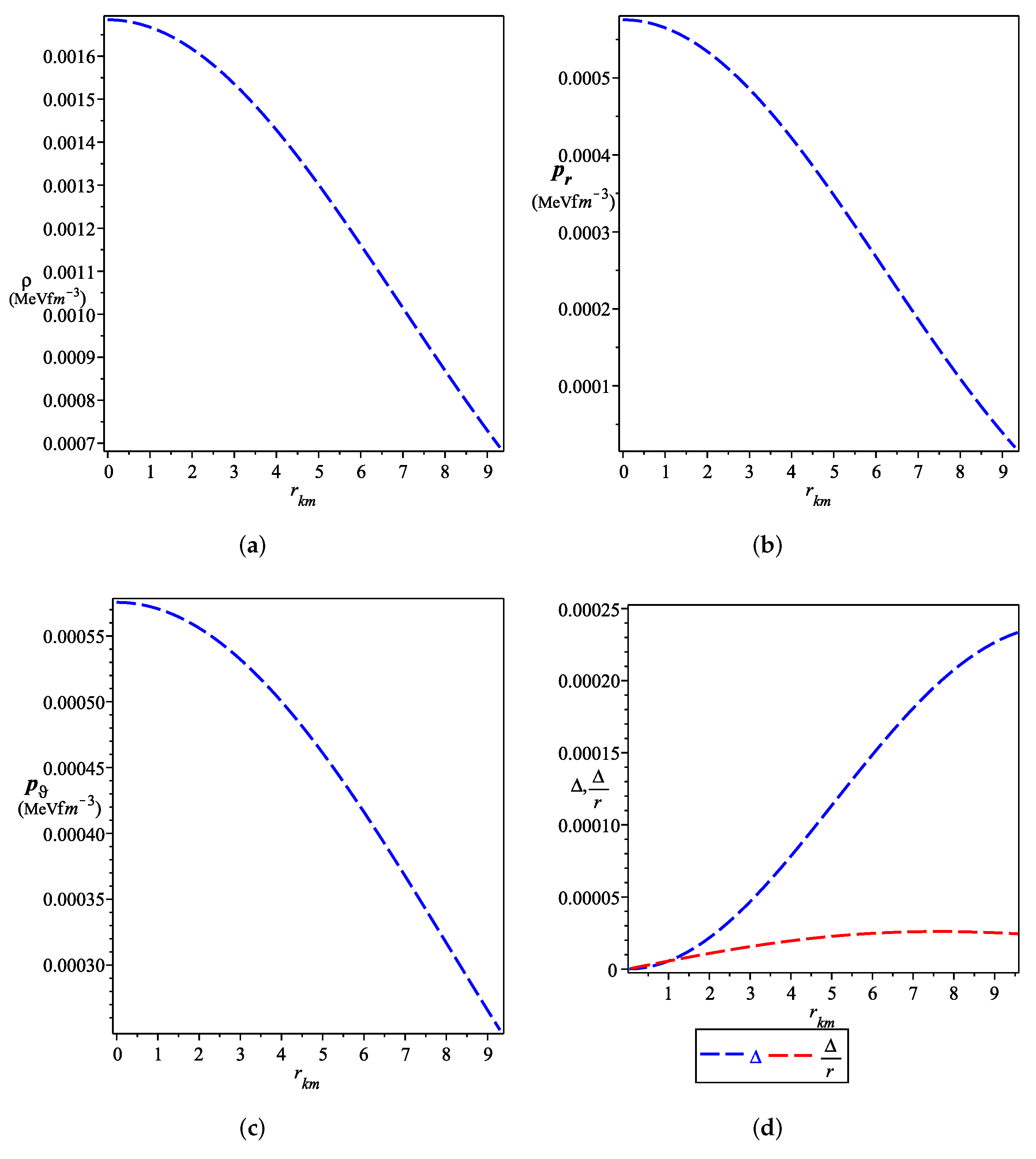
Figure 2.
The plot of the gradients of the energy–momentum components where we put and the constants and take the numerical values, and respectively. (a) The gradient of the energy–momentum components given by the three equations presented Appendix B. (b) The speed of sound given by the two equations presented Appendix C.

Figure 3.
DEC, WEC, NEC, and SEC for , , and . (a) The DEC, and . (b) The WEC, and . (c) The NEC, and . (d) The SEC, , and .
Figure 3.
DEC, WEC, NEC, and SEC for , , and . (a) The DEC, and . (b) The WEC, and . (c) The NEC, and . (d) The SEC, , and .
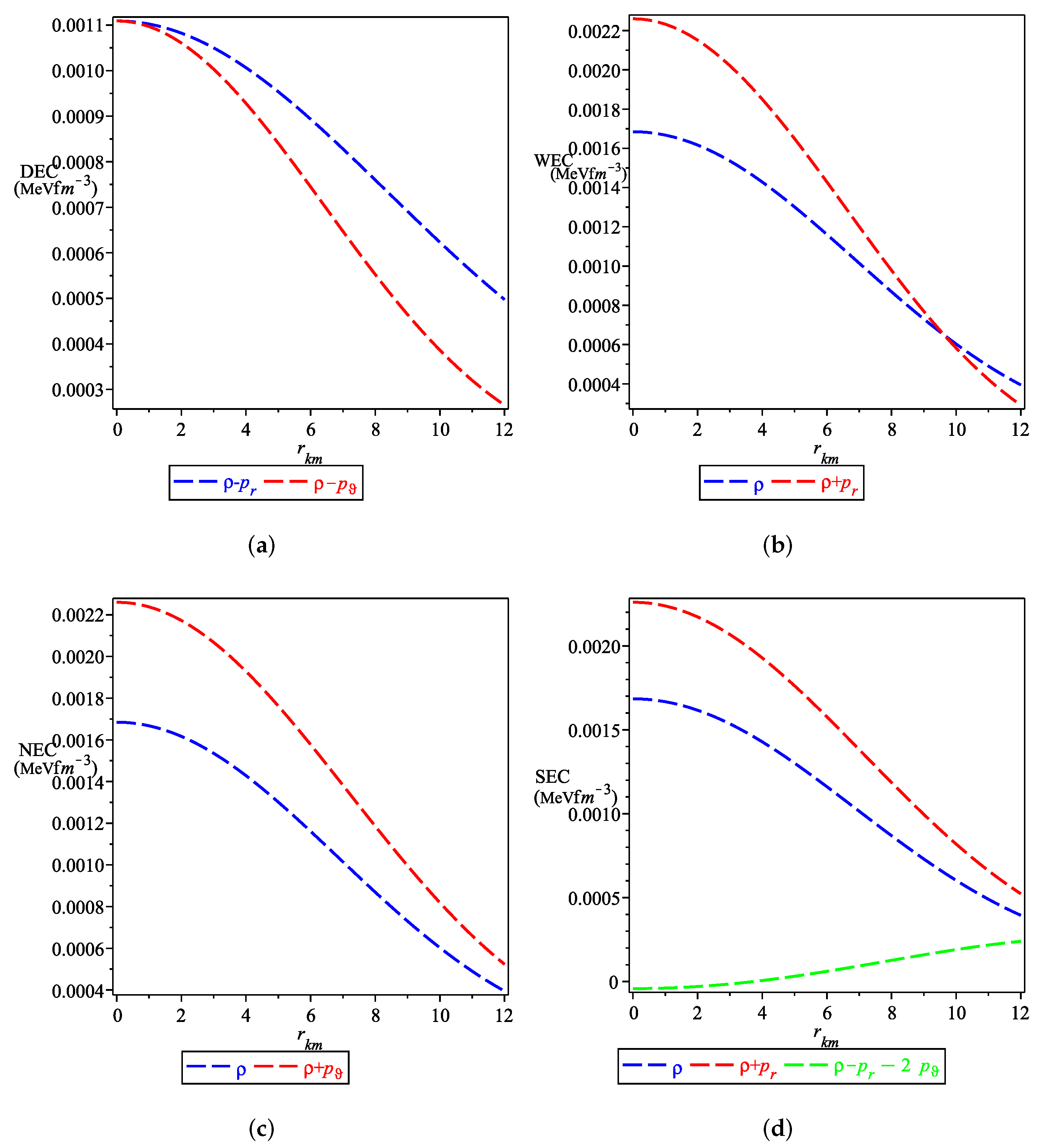
Figure 4.
Schematic plots of (a) the gravitational mass and compactification factor of the solution given by Equations (22) and (23); (b) the components of radial and tangential EoS parameters as function of the radial coordinate; (c) the radial EoS as a function of the energy density; (d) the tangential EoS as a function of the energy density and; (e) the EoS as a function of the energy density. The values the GB parameter and the constants and are taken as , , and in these plots.

Figure 5.
Schematic plots of (a) the different forces acting on the model under consideration; (b) the adiabatic index of the model under consideration; (c) the variation of the mass (which is a function of the central density) via the central density; (d) the stability of the model in the static state. The numerical values of the GB and the constants and used in these plots are given as , , and in this figure.

Table 1.
Values of model parameters [128].
Table 1.
Values of model parameters [128].
| Pulsar | Mass () | Radius (km) | ||
|---|---|---|---|---|
| 4U 1724-207 | ≈ | ≈ | ||
| 4U 1820-30 | ≈ | ≈ | ||
| SAX J1748.9-2021 | ≈ | ≈ | ||
| EXO 1745-268 | ≈ | ≈ | ||
| 4U 1608-52 | ≈ | ≈ | ||
| KS 1731-260 | ≈ | ≈ |
Table 2.
Values of physical quantities.
| Pulsar | |||||||||
|---|---|---|---|---|---|---|---|---|---|
| 4U 1724-207 | ≈0.71 | ≈ 0.32 | ≈ 0.68 | ≈0.57 | ≈ 0.28 | 0.43 | ≈0.42 | ≈0.41 | 0.014 |
| 4U 1820-30 | ≈0.65 | ≈ 0.3 | ≈0.36 | ≈0.26 | ≈0.21 | ≈0.15 | ≈0.58 | ≈0.28 | 0.012 |
| SAX J1748.9-2021 | ≈0.2 | ≈0.6 | ≈0.45 | ≈0.24 | ≈0.26 | ≈0.2 | ≈0.16 | ≈0.35 | ≈0.017 |
| EXO 1745-268 | ≈ 0.1 | ≈0.4 | ≈0.4 | ≈0.27 | ≈0.23 | ≈0.17 | ≈0.8 | ≈0.3 | ≈0.014 |
| 4U 1608-52 | ≈0.1 | ≈0.44 | ≈0.38 | ≈0.25 | ≈0.22 | ≈0.15 | ≈0.92 | ≈0.34 | ≈0.0148 |
| KS 1731-260 | ≈0.1 | ≈ 0.4 | ≈0.15 | ≈0.034 | ≈0.048 | ≈0 | ≈0.1 | ≈0.4 | ≈0.0147 |
Publisher’s Note: MDPI stays neutral with regard to jurisdictional claims in published maps and institutional affiliations. |
© 2022 by the authors. Licensee MDPI, Basel, Switzerland. This article is an open access article distributed under the terms and conditions of the Creative Commons Attribution (CC BY) license (https://creativecommons.org/licenses/by/4.0/).
Share and Cite
MDPI and ACS Style
Nashed, G.G.L.; Odintsov, S.D.; Oikonomou, V.K. Anisotropic Compact Stars in D → 4 Limit of Gauss–Bonnet Gravity. Symmetry 2022, 14, 545. https://doi.org/10.3390/sym14030545
AMA Style
Nashed GGL, Odintsov SD, Oikonomou VK. Anisotropic Compact Stars in D → 4 Limit of Gauss–Bonnet Gravity. Symmetry. 2022; 14(3):545. https://doi.org/10.3390/sym14030545
Chicago/Turabian StyleNashed, Gamal G. L., Sergei D. Odintsov, and Vasillis K. Oikonomou. 2022. "Anisotropic Compact Stars in D → 4 Limit of Gauss–Bonnet Gravity" Symmetry 14, no. 3: 545. https://doi.org/10.3390/sym14030545
Note that from the first issue of 2016, this journal uses article numbers instead of page numbers. See further details here.