
Characterization of Quantum and Classical Critical Points for an Integrable Two-Qubit Spin–Boson Model
by
 , , , and
Roberto Grimaudo
1,*,
Antonino Messina
2 ,
,
Hiromichi Nakazato
3,
Alessandro Sergi
4,5 and
and
Davide Valenti
6
1
Dipartimento di Fisica e Astronomia “E. Majorana", Università degli Studi di Catania, Via S. Sofia 64, I-95123 Catania, Italy
2
Dipartimento di Matematica e Infrormatica, Università degli Studi di Palermo, Via Archirafi 34, I-90123 Palermo, Italy
3
Department of Physics, Waseda University, Tokyo 169-8555, Japan
4
Dipartimento di Scienze Matematiche e Informatiche, Scienze Fisiche e Scienze della Terra, Università degli Studi di Messina, Viale F. Stagno d’Alcontres 31, I-98166 Messina, Italy
5
Institute of Systems Science, Durban University of Technology, P.O. Box 1334, Durban 4000, South Africa
6
Dipartimento di Fisica e Chimica “Emilio Segrè", Università degli Studi di Palermo, Viale delle Scienze, Ed. 18, I-90128 Palermo, Italy
*
Author to whom correspondence should be addressed.
Symmetry 2023, 15(12), 2174; https://doi.org/10.3390/sym15122174
Submission received: 19 October 2023
/
Revised: 24 November 2023
/
Accepted: 5 December 2023
/
Published: 7 December 2023
(This article belongs to the Special Issue Physics and Symmetry Section: Feature Papers 2023)
Abstract
:The class of two-interacting-qubit spin–boson models with vanishing transverse fields on the spin-pair is studied. The model can be mapped exactly into two independent standard single-impurity spin–boson models where the role of the tunneling parameter is played by the spin–spin coupling. The dynamics of the magnetization are analyzed for different levels of (an)isotropy. The existence of a decoherence-free subspace, as well as of different classical regimes separated by a critical temperature, and symptoms of quantum (first-order and Kosterlitz–Thouless type) phase transitions in the Ohmic regime are brought to light.
1. Introduction
The dynamics of any open quantum system is profoundly influenced by its surrounding environment, which is at the origin of decoherence and/or dissipation manifestation [1]. The former effect plays a leading role in determining the transition from quantum to classical behavior. In recent decades, it has attracted much attention, mostly in the field of quantum state manipulation and quantum computation [2].
An important model exhibiting quantum dissipation is the so-called single-impurity spin–boson model (SISBM), which describes a single-spin-1/2 coupled to a bosonic quantum bath [3]. The SISBM has been thoroughly studied in wide regions of the parameter space [3,4,5,6,7,8] with diverse methods and techniques [9,10,11] since 1980. It is a popular starting point for investigations about the dissipative dynamics of a noisy two-level system or qubit. The SISBM indeed encapsulates effects stemming from quantum decoherence, dissipation, and relaxation on the otherwise coherent spin evolution [3]. Furthermore, the model exhibits a nontrivial ground-state behavior since it displays a quantum phase transition as a function of system-bath coupling strength [7,8], attributed to zero-point rather than thermal fluctuations within the bath [12,13,14,15]. Applications are numerous, ranging from quantum optics to quantum information and computation [16,17,18,19,20,21,22,23,24,25,26,27,28,29,30,31,32,33,34,35,36].
The interest towards decoherence and dissipation, as well as quantum phase transitions (QPTs) in two-impurity spin–boson models (TISBMs) with competing interactions, has remarkably grown in the last two decades [37,38,39,40,41,42,43,44,45,46,47,48,49,50]. The TISBM is currently under attention to determine the existence of critical points and then the presence of quantum and/or classical phase transitions [38,39]. Based on numerical approaches, different results have been proposed; however, until now, a univocal response is missing [38,39]. Moreover, a remarkable question to be addressed is whether, in the presence of the impurity-impurity coupling, the transition is of the Kosterlitz–Thouless (K-T) type [38,39].
Recently, a two-qubit quantum Rabi model (QRM), presenting a nontrivial interaction between the two qubits, has been studied [51]. In this case, the qubit–qubit interaction has proved to be fundamental for the determination of two distinguished phases separated by an interaction-based superradiant level-crossing for the ground state of the system [51]. The analogous effect has been brought to light in a more complex system consisting of a two-qubit SBM [52]. There, the authors have found specific and physically meaningful conditions that make the model exactly diagonalizable.
In this work, we analyze the same two-qubit (or two-impurity) SBM, useful for describing binuclear units [53,54], where the transverse (x) field on the spins is absent and a non-isotropic spin–spin Heisenberg interaction is considered. In this case, however, we are interested in investigating the ground-state properties and the dynamical effects of the complex system when the special conditions ensuring the exact solvability are relaxed.
We point out that, until now, the TISBMs considered [37,39,45] have been mainly focused on the effects stemming from the application of external (longitudinal and transverse) magnetic fields, taking into account the simplest spin–spin coupling. In the present work, instead, the attention has been focused on the physical properties of a two-spin/bath system related to the internal parameters that characterize the system itself: a nontrivial spin–spin coupling (anisotropic Heisenberg interaction) and the spin–bath coupling(s). This aspect is of crucial importance from a physical point of view since it means that the results reported in the present work are basically related to the intrinsic nature of the physical system under scrutiny: the two kinds of coupling depend on both the physical geometry of the system and the chemical-physical nature of the constituting elements [53,54]. The physical effects arising from our analysis are then determined by the relative role played by the internal parameters of the system. This kind of study has already shown its potentiality in unveiling intriguing properties of condensed-matter systems coupled to quantized boson field(s) [51,52].
We emphasize that qubit–qubit interactions are fundamental in fields like quantum computation [55,56,57]. In this applicative context [58,59], the generation of multipartite entangled states [55,56,57] can be indeed performed through highly controlled quantum gates [60,61]. Circuit quantum electrodynamics [62,63] and semiconductor systems [64,65,66] are the main scenarios where such a kind of models with spin–spin interaction turns out to be of relevant importance.
Furthermore, the presence of a longitudinal magnetic field is also considered to disclose how such properties are modified when external operations (for example, measurements) are carried out.
We show that the dynamical problem can be exactly and analytically reduced to that of two independent SISBMs, wherein the role of the transverse field is effectively played by the two-spin coupling(s). First, we bring to light the existence of a decoherence-free subspace characterized by dissipationless spin dynamics. Furthermore, based on the results previously obtained for the SISBM in the Ohmic case [3,7,8], we derive the behavior of the magnetization of the system as well as the presence of two classical (non-vanishing temperature) regimes and QPTs. In particular, two types of QPT are present: a first-order QPT (due to a level crossing) and a K-T QPT.
2. Model
The model of two interacting spin-1/2’s subjected to local longitudinal (z) fields and coupled to a common bath of quantum harmonic oscillators can be written (in units of ℏ) as [51,52]:
and () are the characteristic frequencies of the i-th spin and the j-th mode, respectively, while are the parameters taking into account the interaction strength between the i-th spin and the j-th mode. () are the Pauli operators of the spins, while and are the annihilation and creation boson operators of each field mode.
We point out that the present model profoundly differs from those studied until now [37,38,39,40,41,42,43,44,45,46,47,48,49,50]. The latter can be classified as direct generalizations of the single-spin–boson model. These models include indeed both a longitudinal (z) and a transverse (x) magnetic field applied to the spins, the standard interaction term of each spin with the quantum oscillator bath [], and either no spin–spin coupling or (at most) the simplest interaction term () between the two spins. In our model, instead, the transverse (x) field is absent, and a remarkably more complex spin–spin coupling (precisely, an anisotropic Heisenberg interaction) is considered, which has never been proposed and studied so far. This difference between the two types of models is crucial and causes a significantly different physical behavior of the system. The Hamiltonian considered here (see below) is indeed characterized by a symmetry that would be lost if the transverse field were present. We will see, in fact, that this symmetry is the key ingredient, making the model integrable and allowing for the exact reduction of the initial dynamical problem to two independent and easier (sub)problems pertaining to two dynamically invariant subspaces. Moreover, we underline that the transverse spin–boson coupling () is the one usually studied since it can be found and/or implemented in many physical systems. However, the longitudinal one is not unphysical or exotic for physical systems, which can be appropriately exploited for quantum information and quantum computation tasks. It is possible indeed to show that the decoherence mechanism for a qubit (intended as part of a quantum computer) can be formulated in terms of a spin–boson model with a longitudinal spin-mode coupling [67,68,69,70].
Thanks to the existence of the constant of motion , the model can be unitarily transformed into [71] (see Appendix A)
with
where , , [ corresponds to upper (lower) sign], and () is the identity operator in the subspace () which corresponds to the eigenvalue +1 (−1) of the constant of motion . and are then effective Hamiltonians governing the dynamics of the two-spin/bath system (TSBS) within each dynamically invariant subspace, related to each of the two eigenvalues of the constant of motion, and , respectively. In each subspace, the two spins behave as effective two-level systems, so that the two Hamiltonians and can be thought of as the Hamiltonians of two fictitious two-level systems, and , which dynamically arise because of the symmetry exhibited by H (see Appendix A). Indeed, the subspace related to the eigenvalue of is spanned by [with , and ()], and the dynamics is ruled by the effective Hamiltonian (A8). Therefore, in this case, by studying the dynamics of the fictitious two-level system a coupled to its own bath, we study the dynamics of the two-spin/bath system within the subspace . It means that the two states of the fictitious two-level system a are the mapping images of the two two-spin states . Analogously, the subspace related to the eigenvalue of is spanned by , and the effective Hamiltonian ruling the dynamics is given in Equation (A9). In this case, the two two-spin states are mapped into the two states of the fictitious spin-1/2 b. We underline that the dynamical separation allows the easy deriving of the exact time evolution of initial conditions, which have contemporary non-vanishing projections in the two invariant subspaces.
Furthermore, the two independent subdynamics are equivalent to two effective SISBMs: (I) the coupling between the two true spins provides the effective transverse magnetic field ( and ); (II) the longitudinal field results from precise combinations ( and ) of the two fields applied to the actual spin-1/2’s; (III) the coupling with the quantum oscillator bath is mediated by appropriate combinations ( and ) of the coupling parameters of the two-spin-1/2’s with each boson mode. We stress that the field operators appearing in and are formally different. The operator appearing in , in fact, must be intended as . Analogously, in , the same operator is the compact form of the following extended operator . We note that the two effective Hamiltonians are qualitatively similar. However, depending on the specific physical conditions under scrutiny, they can deeply differ and can lead to remarkably different dynamics of the two interacting spins in the two subspaces.
Thanks to our approach, leading to the exactly derived expressions of the two effective Hamiltonians and , we can solve the original two-spin/bath dynamics by solving the two independent effective single-spin–boson subdynamics (see Appendix A). Therefore, all the results obtained for the SISBM can be applied to each subdynamics and exploited to obtain information about the TSBS dynamics.
This last aspect highlights remarkable physical properties directly stemming from the symmetries exhibited by the physical systems. In fact, several physical effects related to the existence of symmetry-protected (sub-)dynamics turn out to be relevant in different contexts, such as quantum metrology [72,73] as well as quantum information and computation [74].
3. Dynamics
3.1. Conditions
Consider the bath in a thermal state and the two-spin system prepared in the state , which is mapped to the fictitious single-spin state ( being the states of the fictitious two-level system a). In this instance, the dynamics are entirely restricted to the subspace and the mean value of the total magnetization , as well as the mean value of the single magnetizations of the two spins, can be easily obtained from (see Appendix B):
The above formula can be easily derived by considering the restrictions of the operators , and to the subspace and that ![Symmetry 15 02174 i001]() (
(![Symmetry 15 02174 i001]() ), , and .
), , and .
 ( ), , and .
In the asymptotic low-temperature limit, the bath spectral density function is determined by the low-energy part of the spectrum and its standard parametrization is
where is a cutoff frequency and is the dimensionless parameter accounting for the dissipation strength [3]. The spectral exponent s defines three regimes: Ohmic (), sub-Ohmic () and super-Ohmic (). We underline that the Ohmic spectral density is imposed on the effective couplings related to the subspace .
3.2. Decoherence-Free Subspace
It is worth noticing that the subspace related to the eigenvalue −1 of (see Appendix A) presents the following peculiar dynamical property. If (both the spin-1/2’s have the same coupling to the bath), implying , the subspace is a decoherence-free subspace. In fact, although the two spins interact with the bath, the fictitious b-spin is effectively decoupled from the quantum oscillator environment. This is due to a sort of ‘compensation’ of the two-spin–bath couplings (i.e., ). This implies that the two actual spins experience dissipationless dynamics within such a subspace as if the bath were absent. Therefore, if the two-spin/bath dynamics occur within such a subspace (this happens if, e.g., the initial condition belongs to such a subspace), the initial or produced entanglement between the spins, would not degrade, despite the presence of the spin–bath coupling term.
This circumstance is of paramount importance in quantum computation, where controlling the dissipative two-spin-boson dynamics in nonequilibrium conditions, e.g., in the presence of time-dependent external fields, is crucial [45,49]. We emphasize that the analytical treatment employed to unitary transform the TISBM is not affected by any time dependence of the Hamiltonian parameters (see Appendix A). In this way, appropriate time variations of the local fields and/or the coupling parameters can be engineered to generate unperturbed quantum gates acting on the two spins.
3.3. Ohmic Regime
The Ohmic case () presents a wide variety of different behaviors depending on the region of the parameter space taken into account [3]. First, consider the case ; this case turns out to be interesting since, in this instance, we can investigate the physical properties of our TISBM, which only depends on the ‘internal’ parameters of the two-spin/bath system, determined by the nature and the geometry [53,54] of the physical system itself: the spin–spin coupling and the spin–bath coupling(s). We underline that all the following results are valid under the conditions below [3]:
and for times large compared to [3].
For the two-spin magnetization reads [3]
This result is valid at all temperatures ( and ) compatible with the condition [3]. The exponential decaying rate of the two-spin probability depends on the ratio , meaning that the characteristic timescale of the system is determined by the spin–spin coupling parameter. Precisely, it depends on the difference , so that: (i) in case of isotropy () the system tends to remain in its initial state; (ii) a slight difference between the two coupling parameters, instead, causes an exponential decay of the magnetization(s) towards the equilibrium value.
For () two cases can be considered [3]:
with
In case (1), the magnetization is [3]
where is the gamma function. The previous expression describes an exponential relaxation with a rate . In case (2): (i) if the time behavior is most likely an incoherent relaxation with an -dependent rate of order ; (ii) if the system exhibits damped incoherent oscillations [3].
These results show that, depending on the ratio of the spin–spin energy coupling to the thermal energy, different dynamics arise. Therefore, the spin–spin interaction, as well as the decaying rate, sets the limit temperature dividing the two dynamical regions. Physical systems characterized by different couplings thus exhibit a different critical temperature and/or different behaviors at the same temperature. Three scenarios can be considered. In nuclear magnetic resonance, the spin–spin coupling typically ranges from 10 Hz to 300 Hz, depending on the molecule [75]. For microwave-driven trapped ions, the interaction strength can reach the kHz range [76]. Rydberg atoms and ions, due to the huge electric-dipole moments of the Rydberg states, are characterized by an effective spin–spin coupling that can reach a few MHz [77,78]. In the three cases the critical temperature separating the two dynamical regimes results , , , respectively. In conclusion, the above considerations show that for dissipative two-spin systems described by the TISBM (1) studied in this work, the spin–spin coupling is crucial for the dynamics of the system since it determines the critical temperature which separates two dynamical regimes characterized by a different evolution of the considered initial condition.
When : (i) if , the two-spin dynamics consists of the same exponential relaxation written in Equation (11), characterized by a rate [3]; (ii) for , instead, the two-spin system experiences the localization regime, i.e., it is frozen in its initial condition [3].
It is worth noticing that all the previous dynamical behaviors rely only on internal parameters characterizing the physical system: the spin–spin coupling, the spin(s)-bath coupling, and the bath cutoff frequency. This aspect suggests a sort of self-organization of the system and an auto-determination of the system dynamics.
An appropriate non-vanishing bias (, ), large compared to the renormalized tunneling frequency (), makes the system to relax from the upper to the lower state, even at zero temperature [3]. Thus, the physical effect of a sufficient bias is to suppress the coherent oscillations shown, in some cases, by the unbiased system. We emphasize that the results reported for can be analytically derived, provided that the physical conditions in Equation (7) are satisfied. The expressions for the case can be obtained instead under the so-called non-interacting-blip approximation, which is essentially a short-time and weak-coupling approximation and becomes exact at high temperatures in the case of an Ohmic bath in the Markovian limit [3].
Mixing Subspaces
All the previous results can even be applied to the subdynamics b, with as the initial state of the two spins and and replaced with and , respectively. Of course, the Hamiltonian parameters are constrained to fulfill and . In this case, net magnetization vanishes, , since .
If we consider the initial condition , both subspaces are involved. In this circumstance, we must independently solve the dynamics in each subspace and ‘merge’ the results. It must be taken into account that the two subdynamics are characterized by different (effective) couplings with the bath and then by different s, say and . Consider the following case: , and . The latter condition stems from , so that .
The time behavior of the net magnetization is determined by the time evolution in the subspace since no contribution stems from the subspace . Therefore, this time, the value of the magnetization is half times that obtained when the system is initially prepared in [Equation (8)].
Rather, a relevant difference is found for and . Previously, we had (Equation (8)). Now, the time behavior of each spin magnetization reads
The cosine term stems from the exact solution of the deterministic dynamics in the subspace .
From Figure 1a,b, we see that the level of anisotropy influences both the frequency of the single-spin oscillations and the decaying rate of the net magnetization. In the case of isotropy (), instead, the two spins exhibit dissipationless oscillations, and the net magnetization is constant [see Figure 1c]. This circumstance is related to the vanishing value of , which rules the exponential relaxation (playing the role of the effective transverse field in the subdynamics a). Therefore, by studying both the oscillation frequency of each spin magnetization and the exponential decaying rate of the net magnetization, the coupling parameters and , and then the level of (an)isotropy of the two-spin system can be estimated.
4. Quantum Phase Transitions
The ground state (GS) of the two-spin system can belong to either the a or b space (coinciding then with the GS of the fictitious spin-qubit a or b) depending on the parameter-space point identified by the Hamiltonian parameters. In this way, we can write the two possible GSs and the related ground energies of the TISBM based on the expressions obtained for the SISBM (see Appendix C). The ansatz proposed in Ref. [8] provides, in the Ohmic case, a good approximation of both the GS and the ground energy of the SISBM in the scaling limit, i.e., in our case, for .
Based on these results, the GS of the TISBM, in the Ohmic regime, takes one of the following forms:
where [8]; stands for the GS of the quantum oscillator bath, ( real) are the bosonic displacement operators, and
with being the normalization factors.
We underline that Equation (19), through the definition of in Equation (17), is self-consistent. However, such a self-consistency is solved by considering the Ohmic spectral density as well as the scaling limit. Indeed, as shown in Ref. [8], under such conditions the equation for can be cast as follows:
where is the Kondo energy which scales the energies of the system, with D being a cutoff introduced to regularize the integral for the ground-state energy [7,8]. We underline that, in our case, the scaling Kondo energy strictly depends on the spin–spin interaction strength.
The related energies can be cast as follows:
Therefore, the spectrum of the TISBM is constituted by two sets of eigenvalues, each of which is the spectrum of the related effective SISBM.
Since the latter does not present level crossing, by studying the difference , the subspace where the GS of the TSBS is placed can be deduced. In Figure 2a the dependence of on for different values of the parameter is shown. The -dependent straight lines emerge by considering the expression of in the limits and , which becomes
The presence of a QPT at is clearly visible, as well as the dependence of the critical point () on k. The GS of the TSBS is then placed in the b (a) space for (). The 2D-plot in Figure 3 shows the two different phases as a function of and k. The white stripe in the figure corresponds to the critical points, i.e., those points where the level crossing occurs.
The critical value , for which such a QPT occurs, is sensitive to the Hamiltonian parameters, as shown in Figure 2b, where . This circumstance can be traced back to the different value taken on in the two cases by the intercept of the straight lines in Equation (23), which is , with the slope remaining unchanged. In the isotropic case (), the QPT is still present since the intercept is .
In the QPT, the spin-pair moves from the vanishing (b) to the non-vanishing (a) magnetization subspace. In this way, the total magnetization plays the role of the order parameter. It jumps from zero to a constant value, which can be derived based on the result obtained for the SISBM, namely [7,8]:
The transition can then be classified as a first-order QPT [12].
When as in Figure 2c, no QPT occurs: the GS of the TSBS is and the net magnetization expression is equal to Equations (24)–(26). This is due to the fact that in this case, can be approximated as in Equation (23), but this time, the intercept takes on the negative value . For homogeneous magnetic fields, (), the QPT is still absent since the intercept reads .
It is worth pointing out that first-order QPTs can occur, in general, in the presence or not of the thermodynamic limit [12]. Within the quantum Rabi model, it is indeed possible to distinguish between fully quantum first-order QPTs that occur at finite frequency ratio(s) and first-order QPTs occurring only for vanishing frequencies for the bosonic field (thermodynamic limit) [79,80,81,82,83]. In these cited works, it is shown that the physical system exhibits physical features related to the ground state remarkably different in the two regimes [79,80,81,82,83].
Now, we discuss the existence of another critical point for , in the limit . For the SISBM in the Ohmic case, indeed, by mapping the model onto the anisotropic Kondo model with bosonization techniques, it has been proved that the K-T transition is present at (in the scaling limit and for vanishing z-magnetic field) [3]. This critical value of separates a localized phase at (the spin is in or ), characterized by a renormalized vanishing tunnel splitting, from a delocalized phase at with an effective non-vanishing tunnel energy [3]. Therefore, based on our approach, we can claim that at the TSBS undergoes a quantum phase transition of the K-T type, with a consequent localization of the two spins in the state or (the fictitious spin-1/2 a localizes in or ). In our case, the tunneling parameter, which renormalizes to 0 for , causing the localization phenomenon, consists of the spin–spin coupling.
We point out that with respect to the previous works [37,39,45], we obtain a different critical value of for which we observe the occurrence of QPTs in the TISBM, e.g., the K-T transition. However, it must be remembered that our TISBM is different from those analyzed to date: the absence of an external actual transverse field applied to the spin-pair is crucial and causes a remarkable difference. The fictitious transverse field that arises in the two effective Hamiltonians governing the two subdynamics of our system is due to the spin–spin coupling, and it is essential for the physical effects discussed here. For this reason, we talk about spin–spin coupling-based QPTs, a phenomenon that is conceptually different from standard QPTs induced by external parameters. In the other works, instead, the physical effects are mainly based on the application of an actual external magnetic field. Due to such a fundamental aspect, the dynamics of our system turn out to be completely different, as well as the results arising from our analysis. The model studied to date [37,39,45] cannot be reduced to that analyzed in our work. Furthermore, if we reduce our model to the one already studied (with a vanishing actual transverse field), we should put the transverse spin–spin coupling equal to zero (). However, it is exactly such a coupling that causes all the intriguing effects highlighted above. Thus, our model is not a particular case of the standard TISBM, and, consequently, our results cannot be obtained by simply considering special conditions on the standard two-spin/bath Hamiltonian [37,39,45]. This circumstance makes our conclusions not comparable with the other ones present in the literature [37,39,45]. Finally, it is worth underlining that the interesting aspects of the present model are both the possibility of rigorously deriving the existence of different classical regimes and quantum phase transitions and the fact that both classical and quantum effects rely on the presence of a non-vanishing transverse spin–spin interaction.
5. Conclusions
The present work reports on nontrivial dynamical effects emerging in a newly proposed two-spin/bath model. Such effects are related to the interplay between the spin–spin coupling and the spin–bath coupling. Until now, the two-spin/bath models considered in the literature [37,39,45] have presented physical effects stemming from the application of external controllable (magnetic) fields, considering only the simplest spin–spin coupling. In our case, instead, the highlighted physical effects are related to the concomitant presence of a nontrivial spin–spin coupling (an anisotropic diagonal dipole interaction or anisotropic Heisenberg interaction) and the standard spin–boson coupling. It means that the physical properties brought to light in our paper depend only on the internal parameters of the system and are then related to the intrinsic nature of a real two-spin/bath system.
The strength and the novelty of our work are grounded in the fact that we have demonstrated that the existing mathematical results valid for the single-qubit spin–boson model (SISBM) can be used in the case of a nontrivial two-qubit spin–boson model (TISBM) to obtain new physical results for the system under scrutiny. The new model proposed here is characterized by an experimentally relevant anisotropic Heisenberg interaction between the two qubits, which supports the occurrence of remarkable dynamic manifestations of entanglement in actual physical qubit systems [55,56,57,58,59,60,61,62,63,64,65,66].
The new physical results established for our TISBM can be summarized as follows: (1) the mathematical expression for the SISBM magnetization is used to derive the TISBM one; (2) the mathematical expressions of the ground state and its energy for the SISBM are the basis to obtain the ground and the first-excited state for the TISBM, which allow us to unravel level crossings and related QPTs; (3) the existence of critical points at non-vanishing temperatures for the SISBM leads us to clearly show the presence of two physical dynamical regimes of the TISBM, which are separated by a critical temperature that, in our case, depends on the spin–spin coupling. This latter aspect transparently discloses the aim of the present work: to bring to light intriguing physical results for a new integrable system smartly exploiting some previous mathematical knowledge. We emphasize that all this is possible only thanks to our analysis and approach, which enables the decomposition of the TISBM dynamics into two independent SISBM dynamics. This fact is another significant result in itself, as it serves as a platform for the whole conceptual construction reported in the manuscript.
We further underline that we have introduced the new concept of spin–spin coupling-based QPTs, which are different from the standard QPTs that are induced by external parameters. In our case, indeed, the parameters playing a role in the QPT are internal physical quantities characterizing the system (the spin mode and the spin–spin couplings). This fact is a crucial point since it means that, depending on the chemical/physical features of a system, the latter can exhibit one phase rather than another. The possible presence of the longitudinal magnetic field allows the consideration of how the physical properties of the TISBM system are modified when external operations (for example, measurements) are carried out.
We highlight that physical systems exist where the internal parameters can be indirectly determined. In dimeric compounds (ensembles of binuclear units), it has been demonstrated that it is possible to enhance the interdimeric interactions with respect to the intradimeric ones [54]. In this case, the single dimeric unit can be described as two spins immersed in a phononic environment constituted by all the other dimeric molecules. Our model (in this case, the modes are phononic excitations) could, therefore, be useful for investigating some of the physical features of such systems.
What deserves to be remarked on is also the fact that our rigorous and exact approach allows the obtaining of analytical results, and, thanks to its generality, it can be applied to other different scenarios and/or other models, opening a wide range of further investigations to better characterize such kind of systems useful for the future quantum technologies. Such an approach is based on the identification of symmetry-induced and symmetry-protected subspaces, thanks to which the dynamical problem can be broken down into relatively easier and treatable (sub)problems, as it happens in different scenarios [84,85,86].
By considering other parameter-space regions, as well as the sub-Ohmic and super-Ohmic regimes, the same approach can lead to a plethora of new results based on those obtained for the SISBM. For example, future works could take into account (I) other results obtained for the SISBM through accurate numerical approaches like HEOM (hierarchical equations of motion) and QUAPI (quasi-adiabatic propagator path integral) methods [11]; (II) different ansatze to the approximate the single-spin–boson ground state, for example, based on superposition of coherent states of the bath [10]. As far as this last point is concerned, we do emphasize that adopting the new ansatze can quantitatively refine the results achieved in this manuscript without significantly countering the existence of QPTs, which is our substantial result. Recently [87], indeed, the comparison between the ansatz we have used here (introduced in Ref. [8]) and the new one [37,87], shows only small deviations in the estimation of the critical parameter(s) (∼0.5% of discrepancy). On this basis, we believe it is reasonable that a superposition of coherent states used as a variational trial of the bath state in the GS of the system would improve the quantitative estimate of the ground-state energy (and its related properties) without conflicting with the existence of the QPT in the physical system under scrutiny.
In future works, possible departures from the integrable scenario can also be considered, which could consist of considering a transverse (along the x direction) external magnetic field and/or a transversal spin-mode coupling. These terms break the symmetry of the Hamiltonian considered in this work, and by considering perturbative approaches, they can create a tunneling between the two subspaces. In this case, it is, therefore, possible to hypothesize that the level crossing would become an avoided crossing with the possible creation of topological excitations in the case of Kibble–Zurek mechanisms [88,89] (that is, the time variation of the control parameter).
Finally, our key idea can be exploited in other formal frameworks too, easily allowing the comparison between different approaches devoted to the dynamical description of open quantum systems: (i) the non-Hermitian formalism [90,91,92,93,94,95,96], (ii) the standard Lindblad theory [97,98], and (iii) the partial Wigner transform [99,100,101,102]. The former, in particular, has been proven to be a mathematical framework suitable for the study and the description of photonic structures, like engineered photonic waveguides, whose possible applications are mainly based on the emergence of quantum-optical analogies (entanglement, Zeno dynamics, Bloch oscillations, etc.) [103,104,105,106] (and references therein).
Author Contributions
Conceptualization, R.G.; methodology, R.G., A.M. and H.N.; validation, A.M., H.N. and D.V.; formal analysis, R.G.; investigation, R.G. and A.M.; writing—original draft preparation, R.G.; writing—review and editing, R.G., A.M., H.N., A.S. and D.V.; visualization, R.G.; supervision, A.M. and D.V.; project administration, A.M. and D.V.; funding acquisition, R.G., H.N. and D.V. All authors have read and agreed to the published version of the manuscript.
Funding
R.G. acknowledges financial support by the PNRR MUR project PE0000023-NQSTI. D.V. acknowledges financial support from the PRIN Project PRJ-0232—Impact of Climate Change on the Biogeochemistry of Contaminants in the Mediterranean Sea (ICCC). H.N. is supported, in part, by the Institute for Advanced Theoretical and Experimental Physics, Waseda University, and by a Waseda University Grant for Special Research Projects (Project No. 2021C-196).
Data Availability Statement
No new data were created or analyzed in this study.
Conflicts of Interest
The authors declare no conflict of interest.
Appendix A. The Model and Its Symmetries
The following model (in units of ℏ)
represents two interacting spin-1/2’s acted upon by local fields along the z direction and coupled to a common bosonic reservoir. , and () are the Pauli matrices.
The Hamiltonian turns out to be invariant under the following transformation [71]
being nothing but a rotation of around the axis of each spin. Therefore, the following unitary operator
with , accomplishes the transformation (A2), and, by construction, it is a constant of motion.
The existence of this constant of motion gives rise to two orthogonal, dynamically invariant, and infinite-dimensional Hilbert subspaces, say and , related to the two eigenvalues of , respectively, and then ( being the total Hilbert space). The two subdynamics living in the two orthogonal subspaces can be extracted by considering that the operator has the same spectrum of ( being the identity operator for the j-th spin), i.e., with the same two-fold degeneracy. Therefore, there exists in a unitary time-independent operator transforming in . The unitary and Hermitian operator
accomplishes the desired transformation:
which in turn allows the transformation of H into , obtaining
Since is a constant of motion of , it can be treated as a parameter and, consequently, can be cast as:
with . This implies the existence of two () subdynamics related to the two dynamically invariant Hilbert subspaces. The two-spin systems, thus, in each dynamically invariant subspace, behave effectively as a two-level system. We may write thus two effective Hamiltonians, each one describing a fictitious two-level system coupled to a bath. In particular, from Equation (A7), when we immediately achieve
while for we obtain
with
The two Hamiltonians must be intended as effective Hamiltonians governing the dynamics of the two-spin/bath system within each dynamically invariant Hilbert subspace, and , respectively. The transformed Hamiltonian can be then written as the direct sum . Thus, the dynamics of the two-spin/bath system in each subspace are equivalent to that of a fictitious single-spin-1/2 immersed in an effective field and coupled to a reservoir through effective coupling constants.
Before concluding, we do remark that the possibility of solving the original problem related to the TISBM is related to two aspects: (1) the decomposition of the total Hilbert space into two invariant subspaces; (2) the possibility of exploiting previous results obtained for the SISBM since the two effective Hamiltonians ( and ), governing the dynamics in the two invariant subspaces, can be mapped into two effective SISBMs where the role of the transverse field is played by the spin–spin coupling.
Appendix B. Observables’ Mapping
Based on the mapping used to write the two effective two-level Hamiltonians and , namely
it is easy to derive the expressions of the two-spin observables in terms of the physical quantities related to the two fictitious TLSs.
First, it is important to point out that the value of is constantly equal to zero in the subspace . Thus, its time evolution depends only on the dynamics within the subspace , and it is easy to verify the following relation
Moreover, following the same reasoning, it is possible to convince oneself that
Since the spin–boson model is invariant under the transformation , then . This implies that, for the two-spin-1/2s, . Therefore, by studying the time evolution of the dynamical variables of the two fictitious TLSs, information about both the dynamical variables and the correlations of the two real spin-1/2s can be easily obtained. Finally, we underline that, as seen before, the value of the operator is constant within each subspace and equal to +1 and −1 for the subspace and , respectively. Then, its value would vanish if initial conditions, consisting of equally weighted superpositions of states belonging to the two subspaces, were considered, e.g., .
Appendix C. Ground State of the Single-Impurity Spin–Boson Model
The ansatz proposed in Ref. [8] provides, in the Ohmic case and in the scaling limit (that is, in our case, for ), a good approximation of both the ground state and its related energy for the single-impurity spin–boson model:
with s assumed real. The ground state and its energy can be written as
where stands for the ground state of the quantum oscillator bath and (with real numbers) are the bosonic displacement operators. The self-consistent equation for , in the scaling limit , reads
where is the Kondo energy which scales the energies of the system, with D being a cutoff introduced to regularize the integral for the ground-state energy [7,8].
References
- Breuer, H.P.; Petruccione, F. The Theory of Open Quantum Systems; Oxford University Press on Demand: Oxford, UK, 2002. [Google Scholar]
- Nielsen, M.A.; Chuang, I.L. Quantum Computation and Quantum Information; Cambridge University Press: Cambridge, UK, 2010. [Google Scholar] [CrossRef]
- Leggett, A.J.; Chakravarty, S.; Dorsey, A.T.; Fisher, M.P.A.; Garg, A.; Zwerger, W. Dynamics of the dissipative two-state system. Rev. Mod. Phys. 1987, 59, 1–85. [Google Scholar] [CrossRef]
- Le Hur, K.; Doucet-Beaupré, P.; Hofstetter, W. Entanglement and Criticality in Quantum Impurity Systems. Phys. Rev. Lett. 2007, 99, 126801. [Google Scholar] [CrossRef] [PubMed]
- Vojta, M.; Tong, N.H.; Bulla, R. Quantum Phase Transitions in the Sub-Ohmic Spin-Boson Model: Failure of the Quantum-Classical Mapping. Phys. Rev. Lett. 2005, 94, 070604. [Google Scholar] [CrossRef] [PubMed]
- Bulla, R.; Tong, N.H.; Vojta, M. Numerical Renormalization Group for Bosonic Systems and Application to the Sub-Ohmic Spin-Boson Model. Phys. Rev. Lett. 2003, 91, 170601. [Google Scholar] [CrossRef] [PubMed]
- Hur, K.L. Entanglement entropy, decoherence, and quantum phase transitions of a dissipative two-level system. Ann. Phys. 2008, 323, 2208–2240. [Google Scholar] [CrossRef]
- Nazir, A.; McCutcheon, D.P.S.; Chin, A.W. Ground state and dynamics of the biased dissipative two-state system: Beyond variational polaron theory. Phys. Rev. B 2012, 85, 224301. [Google Scholar] [CrossRef]
- Winter, A.; Rieger, H.; Vojta, M.; Bulla, R. Quantum Phase Transition in the Sub-Ohmic Spin-Boson Model: Quantum Monte Carlo Study with a Continuous Imaginary Time Cluster Algorithm. Phys. Rev. Lett. 2009, 102, 030601. [Google Scholar] [CrossRef] [PubMed]
- Deng, T.; Yan, Y.; Chen, L.; Zhao, Y. Dynamics of the two-spin spin-boson model with a common bath. J. Chem. Phys. 2016, 144, 144102. [Google Scholar] [CrossRef] [PubMed]
- Wang, L.; Fujihashi, Y.; Chen, L.; Zhao, Y. Finite-temperature time-dependent variation with multiple Davydov states. J. Chem. Phys. 2017, 146, 124127. [Google Scholar] [CrossRef] [PubMed]
- Vojta, M. Quantum phase transitions. Rep. Prog. Phys. 2003, 66, 2069–2110. [Google Scholar] [CrossRef]
- Rossini, D.; Vicari, E. Coherent and dissipative dynamics at quantum phase transitions. Phys. Rep. 2021, 936, 1–110. [Google Scholar] [CrossRef]
- Carollo, A.; Valenti, D.; Spagnolo, B. Geometry of quantum phase transitions. Phys. Rep. 2020, 838, 1–72. [Google Scholar] [CrossRef]
- Carollo, A.; Spagnolo, B.; Dubkov, A.A.; Valenti, D. On quantumness in multi-parameter quantum estimation. J. Stat. Mech. Theory Exp. 2019, 2019, 094010. [Google Scholar] [CrossRef]
- Kundu, S.; Makri, N. Time evolution of bath properties in spin-boson dynamics. J. Phys. Chem. B 2021, 125, 8137–8151. [Google Scholar] [CrossRef] [PubMed]
- Dunnett, A.J.; Chin, A.W. Matrix Product State Simulations of Non-Equilibrium Steady States and Transient Heat Flows in the Two-Bath Spin-Boson Model at Finite Temperatures. Entropy 2021, 23, 77. [Google Scholar] [CrossRef] [PubMed]
- Lemmer, A.; Cormick, C.; Tamascelli, D.; Schaetz, T.; Huelga, S.F.; Plenio, M.B. A trapped-ion simulator for spin-boson models with structured environments. New J. Phys. 2018, 20, 073002. [Google Scholar] [CrossRef]
- Lerma-Hernández, S.; Villaseñor, D.; Bastarrachea-Magnani, M.A.; Torres-Herrera, E.J.; Santos, L.F.; Hirsch, J.G. Dynamical signatures of quantum chaos and relaxation time scales in a spin-boson system. Phys. Rev. E 2019, 100, 012218. [Google Scholar] [CrossRef] [PubMed]
- Leppäkangas, J.; Braumüller, J.; Hauck, M.; Reiner, J.M.; Schwenk, I.; Zanker, S.; Fritz, L.; Ustinov, A.V.; Weides, M.; Marthaler, M. Quantum simulation of the spin-boson model with a microwave circuit. Phys. Rev. A 2018, 97, 052321. [Google Scholar] [CrossRef]
- Puebla, R.; Casanova, J.; Houhou, O.; Solano, E.; Paternostro, M. Quantum simulation of multiphoton and nonlinear dissipative spin-boson models. Phys. Rev. A 2019, 99, 032303. [Google Scholar] [CrossRef]
- Wenderoth, S.; Breuer, H.P.; Thoss, M. Non-Markovian effects in the spin-boson model at zero temperature. Phys. Rev. A 2021, 104, 012213. [Google Scholar] [CrossRef]
- Magazzù, L.; Denisov, S.; Hänggi, P. Asymptotic Floquet states of a periodically driven spin-boson system in the nonperturbative coupling regime. Phys. Rev. E 2018, 98, 022111. [Google Scholar] [CrossRef] [PubMed]
- De Filippis, G.; de Candia, A.; Cangemi, L.M.; Sassetti, M.; Fazio, R.; Cataudella, V. Quantum phase transitions in the spin-boson model: Monte Carlo method versus variational approach à la Feynman. Phys. Rev. B 2020, 101, 180408. [Google Scholar] [CrossRef]
- Wang, Y.Z.; He, S.; Duan, L.; Chen, Q.H. Quantum phase transitions in the spin-boson model without the counterrotating terms. Phys. Rev. B 2019, 100, 115106. [Google Scholar] [CrossRef]
- Wang, Y.Z.; He, S.; Duan, L.; Chen, Q.H. Rich phase diagram of quantum phases in the anisotropic subohmic spin-boson model. Phys. Rev. B 2020, 101, 155147. [Google Scholar] [CrossRef]
- Shen, L.T.; Yang, J.W.; Zhong, Z.R.; Yang, Z.B.; Zheng, S.B. Quantum phase transition and quench dynamics in the two-mode Rabi model. Phys. Rev. A 2021, 104, 063703. [Google Scholar] [CrossRef]
- Aurell, E.; Donvil, B.; Mallick, K. Large deviations and fluctuation theorem for the quantum heat current in the spin-boson model. Phys. Rev. E 2020, 101, 052116. [Google Scholar] [CrossRef]
- Miessen, A.; Ollitrault, P.J.; Tavernelli, I. Quantum algorithms for quantum dynamics: A performance study on the spin-boson model. Phys. Rev. Res. 2021, 3, 043212. [Google Scholar] [CrossRef]
- Villaseñor, D.; Pilatowsky-Cameo, S.; Bastarrachea-Magnani, M.A.; Lerma-Hernández, S.; Santos, L.F.; Hirsch, J.G. Quantum vs classical dynamics in a spin-boson system: Manifestations of spectral correlations and scarring. New J. Phys. 2020, 22, 063036. [Google Scholar] [CrossRef]
- Pino, M.; García-Ripoll, J.J. Quantum annealing in spin-boson model: From a perturbative to an ultrastrong mediated coupling. New J. Phys. 2018, 20, 113027. [Google Scholar] [CrossRef]
- Magazzù, L.; Forn-Díaz, P.; Belyansky, R.; Orgiazzi, J.L.; Yurtalan, M.; Otto, M.R.; Lupascu, A.; Wilson, C.; Grifoni, M. Probing the strongly driven spin-boson model in a superconducting quantum circuit. Nat. Commun. 2018, 9, 1403. [Google Scholar] [CrossRef]
- Lambert, N.; Ahmed, S.; Cirio, M.; Nori, F. Modelling the ultra-strongly coupled spin-boson model with unphysical modes. Nat. Commun. 2019, 10, 3721. [Google Scholar] [CrossRef]
- Casanova, J.; Puebla, R.; Moya-Cessa, H.; Plenio, M.B. Connecting n th order generalised quantum Rabi models: Emergence of nonlinear spin-boson coupling via spin rotations. npj Quantum Inf. 2018, 4, 47. [Google Scholar] [CrossRef]
- Zhou, N.; Chen, L.; Zhao, Y.; Mozyrsky, D.; Chernyak, V.; Zhao, Y. Ground-state properties of sub-Ohmic spin-boson model with simultaneous diagonal and off-diagonal coupling. Phys. Rev. B 2014, 90, 155135. [Google Scholar] [CrossRef]
- Bera, S.; Florens, S.; Baranger, H.U.; Roch, N.; Nazir, A.; Chin, A.W. Stabilizing spin coherence through environmental entanglement in strongly dissipative quantum systems. Phys. Rev. B 2014, 89, 121108. [Google Scholar] [CrossRef]
- Dolgitzer, D.; Zeng, D.; Chen, Y. Dynamical quantum phase transitions in the spin-boson model. Opt. Express 2021, 29, 23988–23996. [Google Scholar] [CrossRef]
- Wang, Y.Z.; He, S.; Duan, L.; Chen, Q.H. Quantum tricritical point emerging in the spin-boson model with two dissipative spins in staggered biases. Phys. Rev. B 2021, 103, 205106. [Google Scholar] [CrossRef]
- Zhou, N.; Zhang, Y.; Lü, Z.; Zhao, Y. Variational Study of the Two-Impurity Spin–Boson Model with a Common Ohmic Bath: Ground-State Phase Transitions. Ann. Der Phys. 2018, 530, 1800120. [Google Scholar] [CrossRef]
- Nägele, P.; Weiss, U. Dynamics of coupled spins in the white- and quantum-noise regime. Phys. E Low-Dimens. Syst. Nanostruct. 2010, 42, 622–628. [Google Scholar] [CrossRef]
- Storcz, M.J.; Hellmann, F.; Hrelescu, C.; Wilhelm, F.K. Decoherence of a two-qubit system away from perfect symmetry. Phys. Rev. A 2005, 72, 052314. [Google Scholar] [CrossRef]
- Garst, M.; Kehrein, S.; Pruschke, T.; Rosch, A.; Vojta, M. Quantum phase transition of Ising-coupled Kondo impurities. Phys. Rev. B 2004, 69, 214413. [Google Scholar] [CrossRef]
- McCutcheon, D.P.S.; Nazir, A.; Bose, S.; Fisher, A.J. Separation-dependent localization in a two-impurity spin-boson model. Phys. Rev. B 2010, 81, 235321. [Google Scholar] [CrossRef]
- Bonart, J. Dissipative phase transition in a pair of coupled noisy two-level systems. Phys. Rev. B 2013, 88, 125139. [Google Scholar] [CrossRef]
- Orth, P.P.; Roosen, D.; Hofstetter, W.; Le Hur, K. Dynamics, synchronization, and quantum phase transitions of two dissipative spins. Phys. Rev. B 2010, 82, 144423. [Google Scholar] [CrossRef]
- Zheng, H.; Lü, Z.; Zhao, Y. Ansatz for the quantum phase transition in a dissipative two-qubit system. Phys. Rev. E 2015, 91, 062115. [Google Scholar] [CrossRef] [PubMed]
- Winter, A.; Rieger, H. Quantum phase transition and correlations in the multi-spin-boson model. Phys. Rev. B 2014, 90, 224401. [Google Scholar] [CrossRef]
- Nägele, P.; Campagnano, G.; Weiss, U. Dynamics of dissipative coupled spins: Decoherence, relaxation and effects of a spin-boson bath. New J. Phys. 2008, 10, 115010. [Google Scholar] [CrossRef]
- Thorwart, M.; Hänggi, P. Decoherence and dissipation during a quantum XOR gate operation. Phys. Rev. A 2001, 65, 012309. [Google Scholar] [CrossRef]
- Storcz, M.J.; Wilhelm, F.K. Decoherence and gate performance of coupled solid-state qubits. Phys. Rev. A 2003, 67, 042319. [Google Scholar] [CrossRef]
- Grimaudo, R.; de Castro, A.S.M.a.; Messina, A.; Solano, E.; Valenti, D. Quantum Phase Transitions for an Integrable Quantum Rabi-like Model with Two Interacting Qubits. Phys. Rev. Lett. 2023, 130, 043602. [Google Scholar] [CrossRef]
- Grimaudo, R.; Valenti, D.; Sergi, A.; Messina, A. Superradiant Quantum Phase Transition for an Exactly Solvable Two-Qubit Spin-Boson Model. Entropy 2023, 25, 187. [Google Scholar] [CrossRef]
- Calvo, R.; Abud, J.E.; Sartoris, R.P.; Santana, R.C. Collapse of the EPR fine structure of a one-dimensional array of weakly interacting binuclear units: A dimensional quantum phase transition. Phys. Rev. B 2011, 84, 104433. [Google Scholar] [CrossRef]
- Napolitano, L.M.B.; Nascimento, O.R.; Cabaleiro, S.; Castro, J.; Calvo, R. Isotropic and anisotropic spin-spin interactions and a quantum phase transition in a dinuclear Cu(II) compound. Phys. Rev. B 2008, 77, 214423. [Google Scholar] [CrossRef]
- Kang, Y.H.; Chen, Y.H.; Wu, Q.C.; Huang, B.H.; Song, J.; Xia, Y. Fast generation of W states of superconducting qubits with multiple Schrödinger dynamics. Sci. Rep. 2016, 6, 36737. [Google Scholar] [CrossRef] [PubMed]
- Lu, M.; Xia, Y.; Song, J.; An, N.B. Generation of N-atom W-class states in spatially separated cavities. J. Opt. Soc. Am. B 2013, 30, 2142–2147. [Google Scholar] [CrossRef]
- Li, J.; Paraoanu, G.S. Generation and propagation of entanglement in driven coupled-qubit systems. New J. Phys. 2009, 11, 113020. [Google Scholar] [CrossRef]
- Barenco, A.; Bennett, C.H.; Cleve, R.; DiVincenzo, D.P.; Margolus, N.; Shor, P.; Sleator, T.; Smolin, J.A.; Weinfurter, H. Elementary gates for quantum computation. Phys. Rev. A 1995, 52, 3457–3467. [Google Scholar] [CrossRef] [PubMed]
- Hua, M.; Tao, M.J.; Deng, F.G. Universal quantum gates on microwave photons assisted by circuit quantum electrodynamics. Phys. Rev. A 2014, 90, 012328. [Google Scholar] [CrossRef]
- Romero, G.; Ballester, D.; Wang, Y.M.; Scarani, V.; Solano, E. Ultrafast Quantum Gates in Circuit QED. Phys. Rev. Lett. 2012, 108, 120501. [Google Scholar] [CrossRef]
- Barends, R.; Quintana, C.M.; Chen, Y.; Kafri, D.; Collins, R.; Naaman, O.; Boixo, S.; Arute, F.; Atya, K.; Buell, D.; et al. Diabatic Gates Frequency-Tunable Supercond Qubits. Phys. Rev. Lett. 2019, 123, 210501. [Google Scholar] [CrossRef] [PubMed]
- Nataf, P.; Ciuti, C. Protected Quantum Computation with Multiple Resonators in Ultrastrong Coupling Circuit QED. Phys. Rev. Lett. 2011, 107, 190402. [Google Scholar] [CrossRef]
- Lizuain, I.; Casanova, J.; García-Ripoll, J.J.; Muga, J.G.; Solano, E. Zeno physics in ultrastrong-coupling circuit QED. Phys. Rev. A 2010, 81, 062131. [Google Scholar] [CrossRef]
- Carusotto, I.; Ciuti, C. Quantum fluids of light. Rev. Mod. Phys. 2013, 85, 299–366. [Google Scholar] [CrossRef]
- Anappara, A.A.; De Liberato, S.; Tredicucci, A.; Ciuti, C.; Biasiol, G.; Sorba, L.; Beltram, F. Signatures of the ultrastrong light-matter coupling regime. Phys. Rev. B 2009, 79, 201303. [Google Scholar] [CrossRef]
- Todorov, Y.; Andrews, A.M.; Colombelli, R.; De Liberato, S.; Ciuti, C.; Klang, P.; Strasser, G.; Sirtori, C. Ultrastrong Light-Matter Coupling Regime with Polariton Dots. Phys. Rev. Lett. 2010, 105, 196402. [Google Scholar] [CrossRef] [PubMed]
- Unruh, W.G. Maintaining coherence in quantum computers. Phys. Rev. A 1995, 51, 992–997. [Google Scholar] [CrossRef] [PubMed]
- Palma, G.M.; Suominen, K.A.; Ekert, A. Quantum computers and dissipation. Proc. R. Soc. London. Ser. A Math. Phys. Eng. Sci. 1996, 452, 567–584. [Google Scholar]
- Morozov, V.G.; Roepke, G. Two-time correlation functions in an exactly solvable spin-boson model. Theor. Math. Phys. 2011, 168, 1271–1277. [Google Scholar] [CrossRef]
- Nesterov, A.I.; Rodríguez Fernández, M.A.; Berman, G.P.; Wang, X. Decoherence as a detector of the Unruh effect. Phys. Rev. Res. 2020, 2, 043230. [Google Scholar] [CrossRef]
- Grimaudo, R.; Nakazato, H.; Messina, A.; Vitanov, N.V. Dzyaloshinskii-Moriya and dipole-dipole interactions affect coupling-based Landau-Majorana-Stückelberg-Zener transitions. Phys. Rev. Res. 2020, 2, 033092. [Google Scholar] [CrossRef]
- Yoshinaga, A.; Tatsuta, M.; Matsuzaki, Y. Entanglement-enhanced sensing using a chain of qubits with always-on nearest-neighbor interactions. Phys. Rev. A 2021, 103, 062602. [Google Scholar] [CrossRef]
- Hatomura, T.; Yoshinaga, A.; Matsuzaki, Y.; Tatsuta, M. Quantum metrology based on symmetry-protected adiabatic transformation: Imperfection, finite time duration, and dephasing. New J. Phys. 2022, 24, 033005. [Google Scholar] [CrossRef]
- Ghiu, I.; Grimaudo, R.; Mihaescu, T.; Isar, A.; Messina, A. Quantum Correlation Dynamics in Controlled Two-Coupled-Qubit Systems. Entropy 2020, 22, 785. [Google Scholar] [CrossRef]
- Vandersypen, L.M.K.; Chuang, I.L. NMR techniques for quantum control and computation. Rev. Mod. Phys. 2005, 76, 1037–1069. [Google Scholar] [CrossRef]
- Weidt, S.; Randall, J.; Webster, S.C.; Lake, K.; Webb, A.E.; Cohen, I.; Navickas, T.; Lekitsch, B.; Retzker, A.; Hensinger, W.K. Trapped-Ion Quantum Logic with Global Radiation Fields. Phys. Rev. Lett. 2016, 117, 220501. [Google Scholar] [CrossRef] [PubMed]
- Gaetan, A.; Miroshnychenko, Y.; Wilk, T.; Chotia, A.; Viteau, M.; Comparat, D.; Pillet, P.; Browaeys, A.; Grangier, P. Observation of collective excitation of two individual atoms in the Rydberg blockade regime. Nat. Phys. 2009, 5, 115–118. [Google Scholar] [CrossRef]
- Urban, E.; Johnson, T.A.; Henage, T.; Isenhower, L.; Yavuz, D.; Walker, T.; Saffman, M. Observation of Rydberg blockade between two atoms. Nat. Phys. 2009, 5, 110–114. [Google Scholar] [CrossRef]
- Ying, Z.J.; Cong, L.; Sun, X.M. Quantum phase transition and spontaneous symmetry breaking in a nonlinear quantum Rabi model. J. Phys. A Math. Theor. 2020, 53, 345301. [Google Scholar] [CrossRef]
- Ying, Z.J. Symmetry-breaking patterns, tricriticalities, and quadruple points in the quantum Rabi model with bias and nonlinear interaction. Phys. Rev. A 2021, 103, 063701. [Google Scholar] [CrossRef]
- Liu, J.; Liu, M.; Ying, Z.J.; Luo, H.G. Fundamental Models in the Light–Matter Interaction: Quantum Phase Transitions and the Polaron Picture. Adv. Quantum Technol. 2021, 4, 2000139. [Google Scholar] [CrossRef]
- Ying, Z.J. From Quantum Rabi Model To Jaynes–Cummings Model: Symmetry-Breaking Quantum Phase Transitions, Symmetry-Protected Topological Transitions and Multicriticality. Adv. Quantum Technol. 2022, 5, 2100088. [Google Scholar] [CrossRef]
- Ying, Z.J. Hidden Single-Qubit Topological Phase Transition without Gap Closing in Anisotropic Light-Matter Interactions. Adv. Quantum Technol. 2022, 5, 2100165. [Google Scholar] [CrossRef]
- Grimaudo, R.; Man’ko, V.I.; Man’ko, M.A.; Messina, A. Dynamics of a harmonic oscillator coupled with a Glauber amplifier. Phys. Scr. 2019, 95, 024004. [Google Scholar] [CrossRef]
- Grimaudo, R.; Vitanov, N.V.; Magalhães de Castro, A.S.; Valenti, D.; Messina, A. Greenberger-Horne-Zeilinger-state Generation in Qubit-Chains via a Single Landau-Majorana-Stückelberg-Zener π/2-pulse. Fortschritte Phys. 2022, 70, 2200010. [Google Scholar] [CrossRef]
- Grimaudo, R.; Magalhães de Castro, A.S.; Messina, A.; Valenti, D. Spin-Chain-Star Systems: Entangling Multiple Chains of Spin Qubits. Fortschritte Phys. 2022, 70, 2200042. [Google Scholar] [CrossRef]
- Qian, X.; Zeng, C.; Zhou, N. Quantum criticality of the Ohmic spin-boson model in a high dense spectrum: Symmetries, quantum fluctuations and correlations. Phys. A Stat. Mech. Its Appl. 2021, 580, 126157. [Google Scholar] [CrossRef]
- Kibble, T.W.B. Topology of cosmic domains and strings. J. Phys. A Math. Gen. 1976, 9, 1387. [Google Scholar] [CrossRef]
- Zurek, W.H. Cosmological experiments in superfluid helium? Nature 1985, 317, 505–508. [Google Scholar] [CrossRef]
- Feshbach, H. Unified theory of nuclear reactions. Ann. Phys. 1958, 5, 357–390. [Google Scholar] [CrossRef]
- Bender, C.M.; Boettcher, S. Real Spectra in Non-Hermitian Hamiltonians Having PT Symmetry. Phys. Rev. Lett. 1998, 80, 5243–5246. [Google Scholar] [CrossRef]
- Mostafazadeh, A. Conceptual aspects of -symmetry and pseudo-Hermiticity: A status report. Phys. Scr. 2010, 82, 038110. [Google Scholar] [CrossRef]
- Rotter, I.; Bird, J.P. A review of progress in the physics of open quantum systems: Theory and experiment. Rep. Prog. Phys. 2015, 78, 114001. [Google Scholar] [CrossRef] [PubMed]
- Sergi, A.; Zloshchastiev, K.G. Non-Hermitian quantum dynamics of a two-level system and model of dissipative environment. Int. J. Mod. Phys. B 2013, 27, 1350163. [Google Scholar] [CrossRef]
- Sergi, A.; Zloshchastiev, K.G. Time correlation functions for non-Hermitian quantum systems. Phys. Rev. A 2015, 91, 062108. [Google Scholar] [CrossRef]
- Brody, D.C.; Graefe, E.M. Mixed-State Evolution in the Presence of Gain and Loss. Phys. Rev. Lett. 2012, 109, 230405. [Google Scholar] [CrossRef] [PubMed]
- Gorini, V.; Kossakowski, A.; Sudarshan, E.C.G. Completely positive dynamical semigroups of N-level systems. J. Math. Phys. 1976, 17, 821–825. [Google Scholar] [CrossRef]
- Lindblad, G. On the generators of quantum dynamical semigroups. Commun. Math. Phys. 1976, 48, 119–130. [Google Scholar] [CrossRef]
- Kapral, R.; Ciccotti, G. Mixed quantum-classical dynamics. J. Chem. Phys. 1999, 110, 8919–8929. [Google Scholar] [CrossRef]
- Kapral, R. Quantum-classical dynamics in a classical bath. J. Phys. Chem. A 2001, 105, 2885–2889. [Google Scholar] [CrossRef]
- Sergi, A. Deterministic constant-temperature dynamics for dissipative quantum systems. J. Phys. A Math. Theor. 2007, 40, F347. [Google Scholar] [CrossRef]
- Sergi, A.; Grimaudo, R.; Hanna, G.; Messina, A. Proposal of a Computational Approach for Simulating Thermal Bosonic Fields in Phase Space. Physics 2019, 1, 402–411. [Google Scholar] [CrossRef]
- Longhi, S. Quantum-optical analogies using photonic structures. Laser Photonics Rev. 2009, 3, 243–261. [Google Scholar] [CrossRef]
- Grimaudo, R.; de Castro, A.S.M.; Kuś, M.; Messina, A. Exactly solvable time-dependent pseudo-Hermitian su(1,1) Hamiltonian models. Phys. Rev. A 2018, 98, 033835. [Google Scholar] [CrossRef]
- Grimaudo, R.; de Castro, A.S.M.; Nakazato, H.; Messina, A. Analytically solvable 2×2PT-symmetry dynamics from su(1,1)-symmetry problems. Phys. Rev. A 2019, 99, 052103. [Google Scholar] [CrossRef]
- Grimaudo, R.; Messina, A.; Sergi, A.; Vitanov, N.V.; Filippov, S.N. Two-Qubit Entanglement Generation through Non-Hermitian Hamiltonians Induced by Repeated Measurements on an Ancilla. Entropy 2020, 22, 1184. [Google Scholar] [CrossRef] [PubMed]
Figure 1.
Time behavior of both the single-spin and the net magnetizations for , , and three levels of isotropy: (a) minimum, (b) intermediate, (c) maximum. The two spins start from , while the bath from the thermal state.
Figure 1.
Time behavior of both the single-spin and the net magnetizations for , , and three levels of isotropy: (a) minimum, (b) intermediate, (c) maximum. The two spins start from , while the bath from the thermal state.
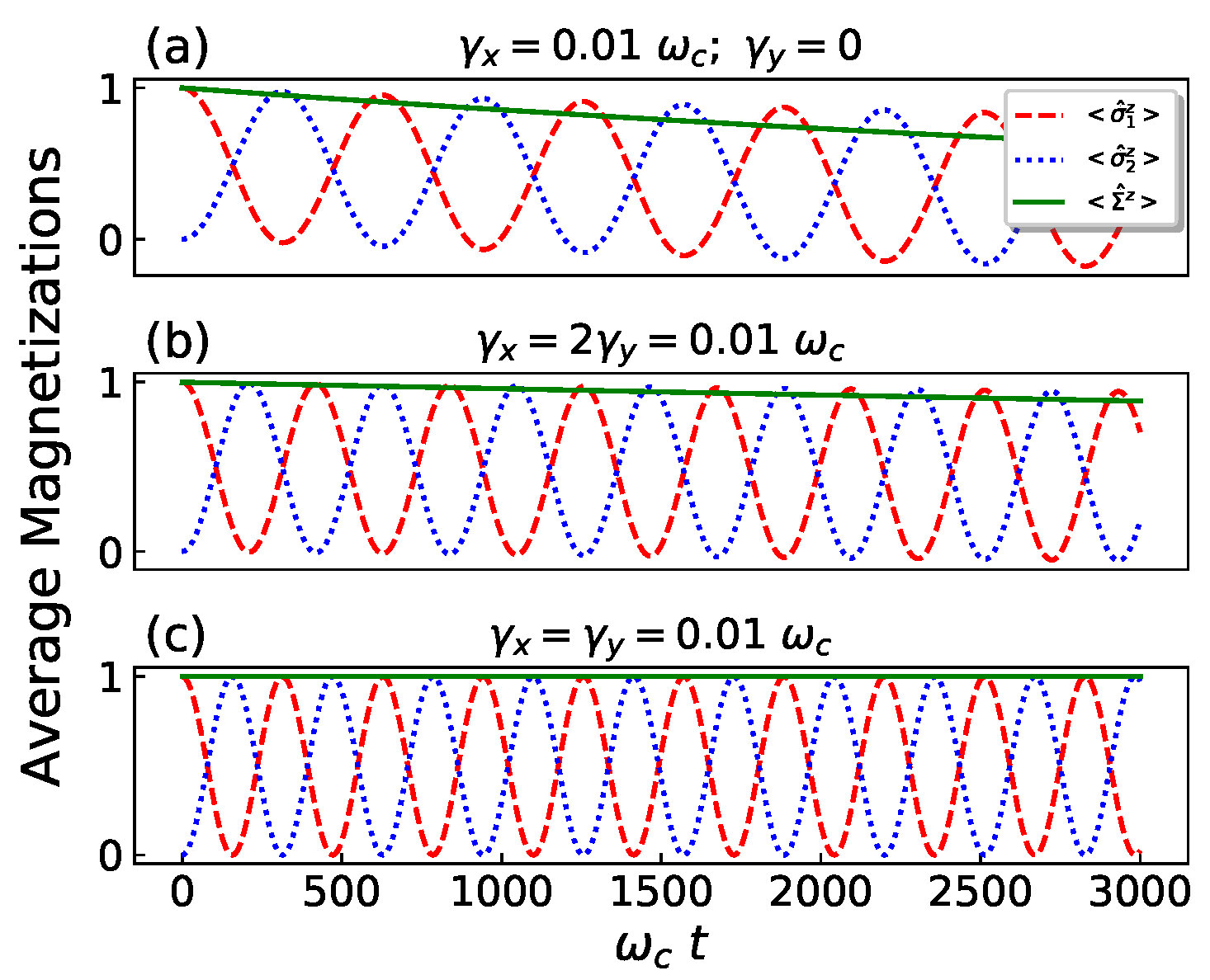
Figure 2.
Dependence of on for: (a) and ; (b) and ; (c) and ; with (solid red line), (dashed green line), (dotted blue line), (dot-dashed cyan line). The horizontal black line represents .
Figure 2.
Dependence of on for: (a) and ; (b) and ; (c) and ; with (solid red line), (dashed green line), (dotted blue line), (dot-dashed cyan line). The horizontal black line represents .
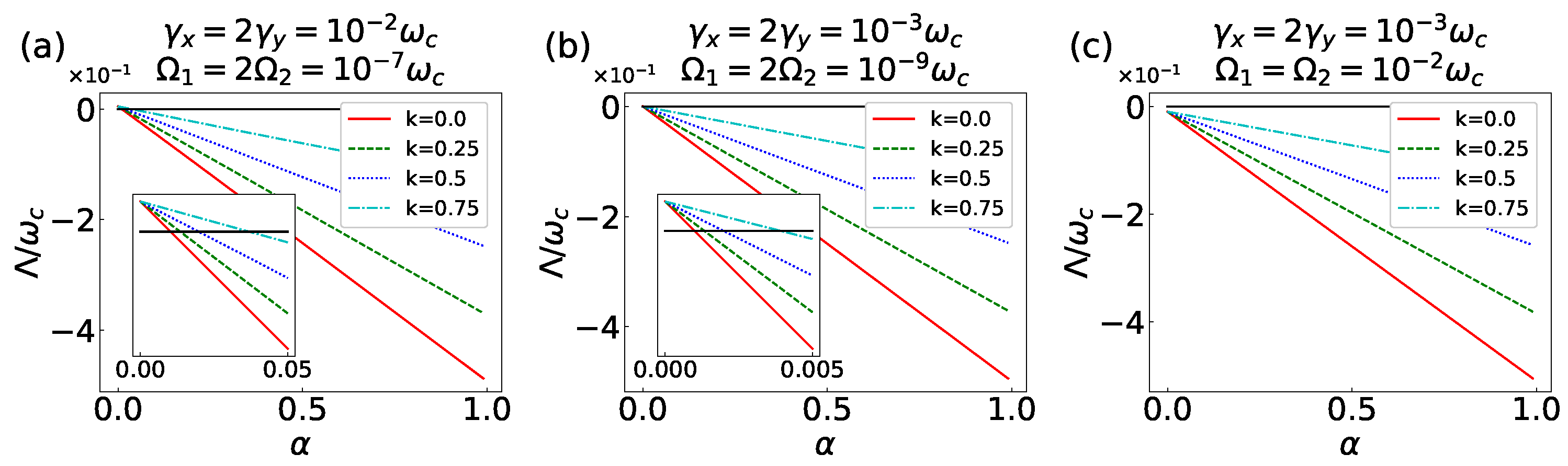
Figure 3.
Dependence of on and k for and . The white strip identifies the critical points where the level crossing occurs. As explicitly shown in the figure, the red (blue) phase corresponds to the GS ().
Figure 3.
Dependence of on and k for and . The white strip identifies the critical points where the level crossing occurs. As explicitly shown in the figure, the red (blue) phase corresponds to the GS ().

Disclaimer/Publisher’s Note: The statements, opinions and data contained in all publications are solely those of the individual author(s) and contributor(s) and not of MDPI and/or the editor(s). MDPI and/or the editor(s) disclaim responsibility for any injury to people or property resulting from any ideas, methods, instructions or products referred to in the content. |
© 2023 by the authors. Licensee MDPI, Basel, Switzerland. This article is an open access article distributed under the terms and conditions of the Creative Commons Attribution (CC BY) license (https://creativecommons.org/licenses/by/4.0/).
Share and Cite
MDPI and ACS Style
Grimaudo, R.; Messina, A.; Nakazato, H.; Sergi, A.; Valenti, D. Characterization of Quantum and Classical Critical Points for an Integrable Two-Qubit Spin–Boson Model. Symmetry 2023, 15, 2174. https://doi.org/10.3390/sym15122174
AMA Style
Grimaudo R, Messina A, Nakazato H, Sergi A, Valenti D. Characterization of Quantum and Classical Critical Points for an Integrable Two-Qubit Spin–Boson Model. Symmetry. 2023; 15(12):2174. https://doi.org/10.3390/sym15122174
Chicago/Turabian StyleGrimaudo, Roberto, Antonino Messina, Hiromichi Nakazato, Alessandro Sergi, and Davide Valenti. 2023. "Characterization of Quantum and Classical Critical Points for an Integrable Two-Qubit Spin–Boson Model" Symmetry 15, no. 12: 2174. https://doi.org/10.3390/sym15122174
Note that from the first issue of 2016, this journal uses article numbers instead of page numbers. See further details here.