Covariant Cubic Interacting Vertices for Massless and Massive Integer Higher Spin Fields

Abstract

We develop the BRST approach to construct the general off-shell local Lorentz covariant cubic interaction vertices for irreducible massless and massive higher spin fields on d-dimensional Minkowski space. We consider two different cases for interacting higher spin fields: with one massive and two massless; two massive, both with coinciding and with different masses and one massless field of spins $s_1,s_2,s_3$. Unlike the previous results on cubic vertices we extend our earlier result in (Buchbinder, I.L.; et al. Phys. Lett. B 2021, 820, 136470) for massless fields and employ the complete BRST operator, including the trace constraints, which is used to formulate an irreducible representation with definite integer spin. We generalize the cubic vertices proposed for reducible higher spin fields in (Metsaev, R.R. Phys. Lett. B 2013, 720, 237) in the form of multiplicative and non-multiplicative BRST-closed constituents and calculate the new contributions to the vertex, which contains the additional terms with a smaller number of space-time derivatives. We prove that without traceless conditions for the cubic vertices in (Metsaev, R.R. Phys. Lett. B 2013, 720, 237) it is impossible to provide the noncontradictory Lagrangian dynamics and find explicit traceless solution for these vertices. As the examples, we explicitly construct the interacting Lagrangians for the massive spin of the s field and the massless scalars, both with and without auxiliary fields. The interacting models with different combinations of triples higher spin fields: massive spin s with massless scalar and vector fields and with two vector fields; massless helicity $\lambda$ with massless scalar and massive vector fields; two massive fields of spins $s, 0$ and massless scalar is also considered.

1. Introduction

The construction of interacting higher spin field theory attracts significant attention both from a general theoretical point of view and in connection with the possibilities of discovering new approaches to describe gravity at the quantum level (see for a review, e.g., [1,2,3,4,5,6,7] and the references therein). The extension of General Relativity on a base of local supersymmetry principle up to the supergravity models [8] with improved quantum properties and a connection with (Super)string Field Theory permits one to include massless fields of spins $s>2$ in Higher Spin Gravity (see [9] and references therein) with respecting the string field theory properties, asymptotic safety and some others. The AdS/CFT correspondence gives strong indications that higher spin excitations can be significant to elaborate the quantum gravity challenges [10]. Interacting massive and massless higher spin fields in constant-curvature spaces provide another possible insight into the origin of Dark Matter and Dark Energy [11,12] beyond the models with vector massive fields [13] and sterile neutrinos [14] to be by reasonable candidates for Dark Matter, see for reviews [15,16,17].

The simplest of higher spin interactions, the cubic vertex for various fields with higher spins, has been studied by many authors with the use of different approaches (see, e.g., the recent papers [18,19,20,21,22,23,24,25,26,27,28,29,30,31] and the references therein) (A complete list of papers on a cubic vertex on constant curvature spaces contains dozens of papers. Here, we cite only the recent papers containing a full list of references). Note, the results on the structure of cubic vertices obtained in terms of physical degrees of freedom in a concise form in the light-cone approach in [31,32]. In the covariant metric-like form, the list of cubic vertices for reducible representations of the Poincare group with discrete spins (being consistent with [32]) are contained in [18], where the cubic vertices were derived using the constrained BRST approach, but without imposing on the vertex the algebraic constraints. The latter peculiarity leads to the violation of the irreducibility of the representation for interacting higher spin fields and, hence, to a possible change of the number of physical degrees of freedom (Without finding the solution for the vertex respecting the algebraic constraints, the number of physical degrees of freedom, which is determined by one of the independent initial data for the equations of motion for the interacting model is different (less) than as one from that for the undeformed model with vanishing algebraic constraints evaluated on respecting equations of motion, but with the deformed gauge symmetry not respecting these constraints). Also, we point out the constructions of cubic vertices within the BRST approach without the use of constraints responsible for trace conditions in the BRST charge (see e.g., [30] and the references therein). It means, in fact, that the vertex is obtained in terms of reducible higher spin fields (To avoid various misunderstandings, we emphasize that we use the term “unconstrained formulation” in the sense that all possible constraints are consequences of the Lagrangian equations of motion. No additional restrictions, separate from the equations of motion, are imposed).

In this paper, we derive the cubic vertices for irreducible massless and massive higher spin fields focusing on the manifest Lorentz covariance. The analysis is carried out within the BRST approach with complete BRST operator that extends our earlier approaches [33,34,35] and involves a converted set of operator constraints forming a first-class gauge algebra. The set of constraints includes on equal-footing the on-shell condition $l_0$ and constraints $l_1,l_{11}$, responsible for divergences and traces. Unlike our consideration, in the constrained BRST approach, the operator $l_{11}$ is imposed as a constraint on the set of fields and gauge parameters outside of the Lagrangian formulation for simplicity of calculations. Such an approach inherits the way of obtaining the Lagrangian formulation for higher spin fields from the tensionless limit [36] for (super)string theory with resulting in a BRST charge without the presence of the algebraic (e.g., trace) constraints. We have already noted [33] that this way of consideration is correct but the actual Lagrangian description of irreducible fields is achieved only after additional imposing the subsidiary conditions which are not derived from the Lagrangian. Of course, the Lagrangian formulations for the same free irreducible higher spin field in Minkowski space obtained in constrained and unconstrained BRST approaches are equivalent [37] (For irreducible massless and massive field representations with half-integer spin the Lagrangians with reducible gauge symmetries and compatible holonomic constraints, were firstly obtained therein). However, the corresponding equivalence has not yet been proved for interacting irreducible higher-spin fields as it was recently demonstrated for massless case [33,34] for cubic vertices. Aspects of the BRST approach with complete BRST operator for a Lagrangian description of various free and interacting massive higher spin field models in Minkowski and AdS spaces were developed in many works (e.g., see the papers [38,39,40,41,42,43,44,45], and the review [3]).

As a result, we face the problem when constructing the cubic vertex for irreducible massless and massive higher integer spin fields on d-dimensional flat space-time within metric-like formalism on the base of the complete BRST operator. It is exactly the problem that we intend to consider in the paper. We expect that the final cubic vertices will contain new terms (as compared with [18]) with the traces of the fields. Such new terms may evidently have significance when gauging away auxiliary gauge symmetry and fields to obtain a component Lagrangian formulation.

The aim of the paper is to present a complete solution of the above problem for the cubic vertices for unconstrained irreducible massless and massive higher spin fields within BRST approach and to obtain from general oscillator-like vertices explicit tensor representations for Lagrangian formulations with reducible gauge symmetry for some triples of interacting higher spin fields.

The paper has the following organization. Section 2 presents the basics of a BRST Lagrangian construction for a free massive higher spin field, with all constraints $l_0,l_1,l_{11}$ taken into account. In Section 3, we deduce a system of equations for a cubic (linear) deformation in fields of the free action (free gauge transformations). A solution for the deformed cubic vertices and gauge transformation is given in a Section 4 for one massive and two massless fields; for two massive with different and coinciding masses and one massless field. The number of examples for the fields with a special set of spins are presented in the Section 5. The main result of the work is that the cubic vertices and deformed reducible gauge transformations include both types of constraints: with derivative $l_1$ and one with trace $l_{11}$. In conclusion, a final summary with comments is given. A derivation of Singh–Hagen Lagrangian from free BRST Lagrangian formulation for the massive field of spin s presented in Appendix A. Appendix B and Appendix C contain results of calculations for component interacting Lagrangian and gauge transformations for massive field of spin s with massless scalars and with massless vector and scalar. In Appendix D we formulate conditions for the incomplete BRST operator, traceless constraints and cubic vertices to obtain non-contradictory Lagrangian dynamics for a model with interacting fields with given spins. We find the form of projectors ${\prod }_{j=1}^3{P}_{0|11}^{\left(j\right)}$ for .respective cubic vertices $|V_c^{\left(3\right)}{\rangle }_{{\left(s\right)}_3}^{{\left(m\right)}_3}$ from [18] to have the cubic vertices $|\overline{V}{}_c^{\left(3\right)}{\rangle }_{{\left(s\right)}_3}^{{\left(m\right)}_3}$, firstly determined by (A66) and (A68) for irreducible interacting fields. We use the usual definitions and notations from the work [33] for a metric tensor ${\eta }_{\mu \nu }=diag(+,-,\dots ,-)$ with Lorentz indices $\mu ,\nu =0,1,\dots ,d-1$ and the respective notation $ϵ\left(F\right)$, $gh\left(F\right)$, $[F,G\}$, $\left[x\right]$, ${\left(s\right)}_3$ for the values of Grassmann parity and ghost number of a homogeneous quantity F, as well as the supercommutator, the integer part of a real-valued x and for the triple $(s_1,s_2,s_3)$.

2. Lagrangian Formulation for Free Massive Higher Spin Fields

Here, we present the basics of the BRST approach to free massive higher integer spin field theory for its following use to construct a general cubic interacting vertex.

The unitary massive irreducible representations of Poincare $ISO(1,d-1)$ group with integer spins s can be realized using the real-valued totally symmetric tensor fields ${\varphi }_{{\mu }_1\dots {\mu }_s}\left(x\right)\equiv {\varphi }_{\mu \left(s\right)}$ subject to the conditions

$$\begin{array}{ccc}\hfill & & \left({\partial }^{\nu }{\partial }_{\nu }+m^2,{\partial }^{{\mu }_1},{\eta }^{{\mu }_1{\mu }_2}\right){\varphi }_{\mu \left(s\right)}=(0,0,0)⟺\hfill \\ & & \left(l_0,l_1,l_{11},g_0-d/2\right)|\varphi \rangle =(0,0,0,s)|\varphi \rangle .\hfill \end{array}$$

(1)

The basic vectors $|\varphi \rangle$ and the operators $l_0,l_1,l_{11},g_0-d/2$ above are defined in the Fock space $\mathcal{H}$ with the Grassmann-even oscillators $a_{\mu },a_{\nu }^{+}$, ($[a_{\mu },a_{\nu }^{+}]=-{\eta }_{\mu \nu }$) as follows

$$\begin{array}{ccc}\hfill & & |\varphi \rangle =\sum _{s\ge 0}\frac{{ı}^s}{s!}{\varphi }^{\mu \left(s\right)}\prod _{i=1}^s{a}_{{\mu }_i}^{+}|0\rangle ,\hfill \\ & & \left(l_0,l_1,l_{11},g_0\right)=({\partial }^{\nu }{\partial }_{\nu }+m^2,-ıa^{\nu }{\partial }_{\nu },\frac{1}{2}{a}^{\mu }{a}_{\mu },-\frac{1}{2}\left\{a_{\mu }^{+},a^{\mu }\right\}).\hfill \end{array}$$

(2)

The free dynamics of the field with definite spin s in the framework of the BRST approach is described by the first-stage reducible gauge theory with the gauge invariant action given on the configuration space $M_{cl}^{\left(s\right)}$ whose dimension grows with the growth of “s”, thus, including the basic field ${\varphi }_{\mu \left(s\right)}$ with many auxiliary fields ${\varphi }_{1\mu (s-1)},\dots$ of lesser than s ranks. All these fields are incorporated into the vector ${|\chi \rangle }_s$ and the dynamics is encoded by the action

$$\begin{array}{c}\hfill {\mathcal{S}}_{0|s}^m[\varphi ,{\varphi }_1,\dots ]={\mathcal{S}}_{0|s}^m{\left[\right|\chi \rangle }_s]=\int d{\eta }_0{}_s{\langle \chi \left|KQ\right|\chi \rangle }_s,\end{array}$$

(3)

where ${\eta }_0$ and K are, respectively, a zero-mode ghost field and an operator defining the inner product. The action (3) is invariant under the reducible gauge transformations

$$\begin{array}{c}\hfill {\delta |\chi \rangle }_s={Q|\mathrm{\Lambda }\rangle }_s{,\delta |\mathrm{\Lambda }\rangle }_s=Q|{\mathrm{\Lambda }}^1{\rangle }_s,\delta {|{\mathrm{\Lambda }}^1\rangle }_s=0,\end{array}$$

(4)

with ${|\mathrm{\Lambda }\rangle }_s$, $|{\mathrm{\Lambda }}^1{\rangle }_s$ to be the vectors of zero-level and first-level gauge parameters of the abelian gauge transformations (4). The quantity Q in (3) is the BRST operator having the same structure as one for massless case [33] constructed on the base of the constraints $l_0,l_1,l{}_1^{+},l{}_{11},l{}_{11}^{+}=\frac{1}{2}{a}^{+\nu }{a}_{\nu }^{+}$ with the Grassmann-odd ghost operators ${\eta }_0,{\eta }_1^{+},{\eta }_1,{\eta }_{11}^{+},{\eta }_{11}$, ${\mathcal{P}}_0$, ${\mathcal{P}}_1$, ${\mathcal{P}}_1^{+},$${\mathcal{P}}_{11},{\mathcal{P}}_{11}^{+},$

$$\begin{array}{ccc}& & Q={\eta }_0{l}_0+{\eta }_1^{+}{\check{l}}_1+{\check{l}}_1^{+}{\eta }_1+{\eta }_{11}^{+}{\widehat{L}}_{11}+{\widehat{L}}_{11}^{+}{\eta }_{11}+ı{\eta }_1^{+}{\eta }_1{\mathcal{P}}_0,\hfill \end{array}$$

(5)

where

$$\begin{array}{ccc}\hfill & & \left({\check{l}}_1,{\check{l}}_1^{+}\right)=\left(l_1+md,l_1^{+}+m{d}^{+}\right),\left({\widehat{L}}_{11},\widehat{L}{}_{11}^{+}\right)=\left({\check{L}}_{11}+{\eta }_1{\mathcal{P}}_1,\check{L}{}_{11}^{+}+{\mathcal{P}}_1^{+}{\eta }_1^{+}\right).\hfill \end{array}$$

(6)

Here

$$\begin{array}{c}\hfill {\check{L}}_{11}=l_{11}-(1/2){\left(d\right)}^2+(b^{+}b+h)b,\check{L}{}_{11}^{+}=l_{11}^{+}-(1/2){\left(d^{+}\right)}^2+b^{+}\end{array}$$

(7)

and $(ϵ,gh)Q=(1,1).$ The algebra of the operators $l_0$, $l_1$, $l_1^{+},{\check{L}}_{11},{\check{L}}_{11}^{+},G_0$ looks like

$$[l_0,l_1^{(+)}]=0,[l_1,l_1^{+}]=l_0-m^2\mathrm{and}[{\check{L}}_{11},{\check{L}}_{11}^{+}]=G_0,[G_0,{\check{L}}_{11}^{+}]=2{\check{L}}_{11}^{+}$$

(8)

and their independent non-vanishing cross-commutators are $[l_1,{\check{L}}_{11}^{+}]=-l_1^{+}$, $[l_1,G_0]=l_1$.

The ghost operators satisfy the non-zero anticommuting relations

$$\{{\eta }_0,{\mathcal{P}}_0\}=ı,\{{\eta }_1,{\mathcal{P}}_1^{+}\}=\{{\eta }_1^{+},{\mathcal{P}}_1\}=\{{\eta }_{11},{\mathcal{P}}_{11}^{+}\}=\{{\eta }_{11}^{+},{\mathcal{P}}_{11}\}=1.$$

(9)

The theory is characterized by the spin operator $\sigma$, which is defined according to

$$\begin{array}{ccc}\hfill & & \sigma =G_0+{\eta }_1^{+}{\mathcal{P}}_1-{\eta }_1{\mathcal{P}}_1^{+}+2({\eta }_{11}^{+}{\mathcal{P}}_{11}-{\eta }_{11}{\mathcal{P}}_{11}^{+})\hfill \\ \hfill & & G_0=g_0+d^{+}d+2b^{+}b+\frac{1}{2}+h.\hfill \end{array}$$

(10)

Here, $d,d^{+}$, $b,b^{+}$ ($[d,d^{+}]=1$, $[b,b^{+}]=1$) are two pairs of auxiliary Grassmann-even oscillators. The operator $\sigma$ selects the vectors with definite spin value s

$$\begin{array}{ccc}\hfill & & \sigma {\left(\right|\chi \rangle }_s{,|\mathrm{\Lambda }\rangle }_s,|{\mathrm{\Lambda }}^1{\rangle }_s)=(0,0,0),\hfill \end{array}$$

(11)

where the standard distribution for Grassmann parities and the ghost numbers of these vectors are $(0,0)$, $(1,-1),$$(0,-2)$, respectively.

All the operators above act in a total Hilbert space with the scalar product of the vectors depending on all oscillators $(A;A^{+})$ = $(a^{\mu },b,d;a^{\mu +},b^{+},d^{+})$ and ghosts

$$\begin{array}{ccc}& & \langle \chi |\psi \rangle =\int d^{d}x\langle 0|{\chi }^{*}\left(A;{\eta }_0,{\eta }_1,{\mathcal{P}}_1,{\eta }_{11},{\mathcal{P}}_{11}\right)\psi \left(A^{+};{\eta }_0,{\eta }_1^{+},{\mathcal{P}}_1^{+},{\eta }_{11}^{+},{\mathcal{P}}_{11}^{+}\right)|0\rangle .\hfill \end{array}$$

(12)

The operators $Q, \sigma$ are supercommuting and Hermitian with respect to the scalar product (12) including the operator K (see e.g., [37,39,45]) being equal to 1 on Hilbert subspace not depending on auxiliary $b,b^{+}$ operators

$$\begin{array}{cc}{Q}^2={\eta }_{11}^{+}{\eta }_{11}\sigma ,\hfill & [Q,\sigma \}=0;\hfill \end{array}$$

(13)

$$\begin{array}{cc}{Q}^{+}K=KQ,\hfill & {\sigma }^{+}K=K\sigma ,\hfill \end{array}$$

(14)

$$\begin{array}{cc}K=1\otimes \sum _{n=0}^{\infty }\frac{1}{n!}\left(b^{+}\right)n|0\rangle \langle 0|b^{n}C(n,h\left(s\right)),\hfill & C(n,h\left(s\right))\equiv \prod _{i=0}^{n-1}(i+h\left(s\right))\hfill \end{array}$$

(15)

The BRST operator Q is nilpotent on the subspace with zero eigenvectors for the spin operator $\sigma$ (11).

The field ${|\chi \rangle }_s$, the zero ${|\mathrm{\Lambda }\rangle }_s$ and the first $|{\mathrm{\Lambda }}^1{\rangle }_s$ level gauge parameters labeled by the symbol $“s”$ as eigenvectors of the spin condition in (11) has the same decomposition as ones in [33] but with ghost-independent vectors $|{\mathrm{\Phi }}_{\dots }{\rangle }_{s-\dots }$, $|{\mathrm{\Xi }}_{\dots }{\rangle }_{s-\dots }$ instead of $|{\varphi }_{\dots }{\rangle }_{s-\dots }$, $|{\mathrm{\Xi }}_{\dots }{\rangle }_{s-\dots }$

$$\begin{array}{ccc}\hfill & & {|\chi \rangle }_s={|\mathrm{\Phi }\rangle }_s+{\eta }_1^{+}\left({\mathcal{P}}_1^{+}|{\mathrm{\Phi }}_2{\rangle }_{s-2}+{\mathcal{P}}_{11}^{+}|{\mathrm{\Phi }}_{21}{\rangle }_{s-3}+{\eta }_{11}^{+}{\mathcal{P}}_1^{+}{\mathcal{P}}_{11}^{+}{|{\mathrm{\Phi }}_{22}\rangle }_{s-6}\right)\hfill \\ \hfill & & \phantom{|{\chi }_c^0{\rangle }_s}+{\eta }_{11}^{+}\left({\mathcal{P}}_1^{+}|{\mathrm{\Phi }}_{31}{\rangle }_{s-3}+{\mathcal{P}}_{11}^{+}{|{\mathrm{\Phi }}_{32}\rangle }_{s-4}\right)+{\eta }_0({\mathcal{P}}_1^{+}|{\mathrm{\Phi }}_1{\rangle }_{s-1}+{\mathcal{P}}_{11}^{+}{|{\mathrm{\Phi }}_{11}\rangle }_{s-2}\hfill \\ \hfill & & \phantom{|{\chi }_c^0{\rangle }_s}+{\mathcal{P}}_1^{+}{\mathcal{P}}_{11}^{+}\left[{\eta }_1^{+}|{\mathrm{\Phi }}_{12}{\rangle }_{s-4}+{\eta }_{11}^{+}{|{\mathrm{\Phi }}_{13}\rangle }_{s-5}\right]),\hfill \end{array}$$

(16)

$$\begin{array}{ccc}\hfill & & {|\mathrm{\Lambda }\rangle }_s={\mathcal{P}}_1^{+}{|\mathrm{\Xi }\rangle }_{s-1}+{\mathcal{P}}_{11}^{+}|{\mathrm{\Xi }}_1{\rangle }_{s-2}+{\mathcal{P}}_1^{+}{\mathcal{P}}_{11}^{+}({\eta }_1^{+}{|{\mathrm{\Xi }}_{11}\rangle }_{s-4}\hfill \\ \hfill & & \phantom{|{\chi }^1{\rangle }_s}+{\eta }_{11}^{+}|{\mathrm{\Xi }}_{12}{\rangle }_{s-5})+{\eta }_0{\mathcal{P}}_1^{+}{\mathcal{P}}_{11}^{+}{|{\mathrm{\Xi }}_{01}\rangle }_{s-3},\hfill \end{array}$$

(17)

$$\begin{array}{ccc}\hfill & & |{\mathrm{\Lambda }}^1{\rangle }_s={\mathcal{P}}_1^{+}{\mathcal{P}}_{11}^{+}{|{\mathrm{\Xi }}^1\rangle }_{s-3}.\hfill \end{array}$$

(18)

Here,

$$\begin{array}{ccc}\hfill |{\mathrm{\Phi }}_{\dots }{\rangle }_{s-\dots }& =& \sum _{l=0}^{[s-../2]-l}\frac{{\left(b^{+}\right)}^l}{l!}\sum _{k=0}^{s-2l\dots }\frac{{\left(d^{+}\right)}^k}{k!}|{\varphi }_{\dots |l,k}\left(a^{+}\right){\rangle }_{s-k-2l\dots },\mathrm{for}|{\varphi }_{|0,0}\left(a^{+}\right){\rangle }_s\equiv {|\varphi \rangle }_s,\hfill \end{array}$$

(19)

$$\begin{array}{ccc}\hfill |{\mathrm{\Xi }}_{\dots }{\rangle }_{s-\dots }& =& \sum _{l=0}^{[s-\dots /2]-l}\frac{{\left(b^{+}\right)}^l}{l!}\sum _{k=0}^{s-2l\dots }\frac{{\left(d^{+}\right)}^k}{k!}{|{\mathrm{\Xi }}_{\dots |l,k}\left(a^{+}\right)\rangle }_{s-k-2l\dots }.\hfill \end{array}$$

(20)

We prove in the Appendix A that after imposing the appropriate gauge conditions and eliminating the auxiliary fields with help of the equations of motion, the theory under consideration is reduced to Singh–Hagen ungauged form [46] in terms of a totally symmetric double traceless tensor field ${\varphi }^{\mu \left(s\right)}$ and auxiliary traceless ${\varphi }_3^{\mu (s-3)}$.

Now we turn to the interacting theory.

3. System of Equations for Cubic Vertex

Here, we follow the general scheme developed for massless case in [33] to find the cubic interaction vertices for the models with one massive and two massless higher spin fields, two massive and one massless higher spin field with different mass value distributions and derive the equations for these vertices.

To include the cubic interaction we introduce three vectors $|{\chi }^{\left(i\right)}{\rangle }_{s_i}$, gauge parameters $|{\mathrm{\Lambda }}^{\left(i\right)}{\rangle }_{s_i}$, $|{\mathrm{\Lambda }}^{\left(i\right)1}{\rangle }_{s_i}$ with corresponding vacuum vectors ${|0\rangle }^i$ and oscillators, where $i=1,2,3$. It permits to define the deformed action and the deformed gauge transformations as follows

$$\begin{array}{ccc}\hfill & & S_{{\left[1\right]|\left(s\right)}_3}^{{\left(m\right)}_3}[{\chi }^{\left(1\right)},{\chi }^{\left(2\right)},{\chi }^{\left(3\right)}]=\sum _{i=1}^3{\mathcal{S}}_{0|s_i}^{m_i}+g\int \prod _{e=1}^{3}d{\eta }_0^{\left(e\right)}\left({}_{s_e}{\langle {\chi }^{\left(e\right)}{K}^{\left(e\right)}|V^{\left(3\right)}\rangle }_{{\left(s\right)}_3}^{{\left(m\right)}_3}+h.c.\right),\hfill \end{array}$$

(21)

$$\begin{array}{ccc}& & {\delta }_{\left[1\right]}|{\chi }^{\left(i\right)}{\rangle }_{s_i}=Q^{\left(i\right)}|{\mathrm{\Lambda }}^{\left(i\right)}{\rangle }_{s_i}-g\int \prod _{e=1}^{2}d{\eta }_0^{(i+e)}({}_{s_{i+1}}\langle {\mathrm{\Lambda }}^{\left(i+1\right)}{K}^{(i+1)}|{}_{s_{i+2}}\langle {\chi }^{\left(i+2\right)}{K}^{(i+1)}|\hfill \\ & & \phantom{{\delta }_{\left[1\right]}|{\chi }^{\left(i\right)}{\rangle }_{s_i}}+(i+1\leftrightarrow i+2)\left)\right|\tilde{V}{}^{\left(3\right)}{\rangle }_{{\left(s\right)}_3}^{{\left(m\right)}_3},\hfill \end{array}$$

(22)

$$\begin{array}{ccc}& & {\delta }_{\left[1\right]}|{\mathrm{\Lambda }}^{\left(i\right)}{\rangle }_{s_i}=Q^{\left(i\right)}|{\mathrm{\Lambda }}^{\left(i\right)1}{\rangle }_{s_i}-g\int \prod _{e=1}^{2}d{\eta }_0^{(i+e)}({}_{s_{i+1}}\langle {\mathrm{\Lambda }}^{(i+1)1}{K}^{(i+1)}|{}_{s_{i+2}}\langle {\chi }^{\left(i+2\right)}{K}^{(i+1)}|\hfill \\ & & \phantom{{\delta }_{\left[1\right]}|{\chi }^{\left(i\right)}{\rangle }_{s_i}}+(i+1\leftrightarrow i+2))|\widehat{V}{}^{\left(3\right)}{\rangle }_{{\left(s\right)}_3}^{{\left(m\right)}_3}\hfill \end{array}$$

(23)

with some unknown three-vectors $|V^{\left(3\right)}{\rangle }_{{\left(s\right)}_3}^{{\left(m\right)}_3},|\tilde{V}{}^{\left(3\right)}{{\rangle }_{{\left(s\right)}_3}^{{\left(m\right)}_3},|\widehat{V}{}^{\left(3\right)}\rangle }_{{\left(s\right)}_3}^{{\left(m\right)}_3}.$ Here, ${\mathcal{S}}_{0|s_i}^{m_i}$ is the free action (3) for the field $|{\chi }^{\left(i\right)}{\rangle }_{s_i}$, $Q^{\left(i\right)}$ is the BRST charge corresponding to spin $s_i,i=1,2,3$, $K^{\left(i\right)}$ is the operator K (15) corresponding to spin $s_i,i=1,2,3$ for massive and with change $h\left(s\right)\to h\left(s\right)+1/2$ for massless field and g is a deformation parameter (called usually as a coupling constant). Also, we use the notation ${\left(m\right)}_3\equiv (m_1,m_2,m_3)$ and convention $[i+3\simeq i]$.

The concrete construction of the cubic interaction means finding the concrete vectors $|V^{\left(3\right)}{\rangle }_{{\left(s\right)}_3}^{{\left(m\right)}_3}$, $|\tilde{V}{}^{\left(3\right)}{\rangle }_{{\left(s\right)}_3}^{{\left(m\right)}_3}$, $|\widehat{V}{}^{\left(3\right)}{\rangle }_{{\left(s\right)}_3}^{{\left(m\right)}_3}$. For this purpose, we can involve the set of fields, the constraints, and ghost operators related with spins $s_1,s_2,s_3$ and the respective conditions of gauge invariance of the deformed action under the deformed gauge transformations as well as the conservation of the form of the gauge transformations for the fields $|{\chi }^{\left(i\right)}{\rangle }_{s_i}$ under the gauge transformations ${\delta }_{\left[1\right]}|{\mathrm{\Lambda }}^{\left(i\right)}{\rangle }_{s_i}$ at the first power in g (In this connection, note also the results of recent works [47,48,49,50] obtained on the base of the deformation of general gauge theory [51,52,53,54]).

$$\begin{array}{ccc}& & g\int \prod _{e=1}^{3}d{\eta }_0^{\left(e\right)}{}_{s_j}\langle {\mathrm{\Lambda }}^{\left(j\right)}{K}^{\left(j\right)}|{}_{s_{j+1}}\langle {\chi }^{(j+1)}{K}^{(j+1)}|{}_{s_{j+2}}\langle {\chi }^{(j+2)}{K}^{(j+2)}|\mathcal{Q}(V^3,{\tilde{V}}^3)=0,\hfill \end{array}$$

(24)

$$\begin{array}{ccc}& & g\int \prod _{e=1}^{2}d{\eta }_0^{\left(e\right)}{}_{s_{j+1}}\langle {\mathrm{\Lambda }}^{(j+1)1}{K}^{(j+1)}|{}_{s_{j+2}}\langle {\chi }^{(j+2)}{K}^{(j+2)}|\left(\mathcal{Q}({\tilde{V}}^3,{\widehat{V}}^3)-Q^{(j+2)}|\widehat{V}{}^{\left(3\right)}\rangle \right)=0,\hfill \end{array}$$

(25)

where

$$\begin{array}{ccc}\hfill \phantom{g^1:}& & \mathcal{Q}(V^3,{\tilde{V}}^3)=\sum _{k=1}^3{Q}^{\left(k\right)}|\tilde{V}{}^{\left(3\right)}{\rangle }_{{\left(s\right)}_3}^{{\left(m\right)}_3}+Q^{\left(j\right)}\left(|V{}^{\left(3\right)}{{\rangle }_{{\left(s\right)}_3}^{{\left(m\right)}_3}-|\tilde{V}{}^{\left(3\right)}\rangle }_{{\left(s\right)}_3}^{{\left(m\right)}_3}\right),j=1,2,3.\hfill \end{array}$$

(26)

Following our results, [33,34] we choose coincidence for the vertices: $|\tilde{V}{}^{\left(3\right)}\rangle$ = $|V{}^{\left(3\right)}\rangle$ = $|\widehat{V}{}^{\left(3\right)}\rangle$, which provides the validity of the operator equations at the first order in g (the highest orders are necessary for finding the quartic and higher vertices)

$$Q^{tot}|V{}^{\left(3\right)}{{\rangle }_{{\left(s\right)}_3}^{{\left(m\right)}_3}=0,{\sigma }^{\left(i\right)}|V{}^{\left(3\right)}\rangle }_{{\left(s\right)}_3}^{{\left(m\right)}_3}=0,$$

(27)

jointly with the spin conditions as the consequence of the spin Equation (11) for each sample (with $|{\chi }^{\left(i\right)}{\rangle }_{s_i},|{\mathrm{\Lambda }}^{\left(i\right)}{\rangle }_{s_i},{|{\mathrm{\Lambda }}^{\left(i\right)1}\rangle }_{s_i}$) providing the nilpotency of total BRST operator $Q^{tot}\equiv {\sum }_i{Q}^{\left(i\right)}$ when evaluated on the vertex due to the Equations (13) and $\{Q^{\left(i\right)},Q^{\left(j\right)}\}=0$ for $i\ne j$.

A local dependence on space-time coordinates in the vertices $|V^{\left(3\right)}\rangle$, $|\tilde{V}{}^{\left(3\right)}\rangle$, $|\widehat{V}{}^{\left(3\right)}\rangle$ means

$$|V^{\left(3\right)}{\rangle }_{{\left(s\right)}_3}^{{\left(m\right)}_3}=\prod _{i=2}^3{\delta }^{\left(d\right)}\left(x_1-x_i\right)V^{\left(3\right)|}{}_{{\left(s\right)}_3}^{{\left(m\right)}_3}\prod _{j=1}^3{\eta }_0^{\left(j\right)}|0\rangle ,|0\rangle \equiv {\otimes }_{e=1}^3{|0\rangle }^e$$

(28)

(for $(ϵ,gh)V^{\left(3\right)|}{}_{{\left(s\right)}_3}^{{\left(m\right)}_3}=(0,0)$). We have the conservation law: ${\sum }_{i=1}^3{p}_{\mu }^{\left(i\right)}=0$, for the momenta associated with all vertices. Again as for the massless case [33], the deformed gauge transformations still form the closed algebra, that means after the simple calculations

$$\begin{array}{ccc}& & \left[{\delta }_{\left[1\right]}^{{\mathrm{\Lambda }}_1},{\delta }_{\left[1\right]}^{{\mathrm{\Lambda }}_2}\right]|{\chi }^{\left(i\right)}\rangle =-g{\delta }_{\left[1\right]}^{{\mathrm{\Lambda }}_3}|{\chi }^{\left(i\right)}\rangle ,\hfill \\ & & |{\mathrm{\Lambda }}_3\rangle \sim \int \prod _{e=1}^{2}d{\eta }_0^{(i+e)}\left(\langle {\mathrm{\Lambda }}_2^{(i+1)}K|\langle {\mathrm{\Lambda }}_1^{(i+2)}|K+\left(i+1\leftrightarrow i+2\right)\right)-\left({\mathrm{\Lambda }}_1\leftrightarrow {\mathrm{\Lambda }}_2\right)\}|V{}^{\left(3\right)}\rangle \hfill \end{array}$$

(29)

with the Grassmann-odd gauge parameter ${\mathrm{\Lambda }}_3$ being a function of the parameters ${\mathrm{\Lambda }}_1,{\mathrm{\Lambda }}_2,$${\mathrm{\Lambda }}_3={\mathrm{\Lambda }}_3({\mathrm{\Lambda }}_1,{\mathrm{\Lambda }}_2)$.

The Equations (27) (for coinciding vertices $V{}^{\left(3\right)}=\tilde{V}{}^{\left(3\right)}=\widehat{V}{}^{\left(3\right)}$) together with the form of the commutator of the gauge transformations (29) determine the cubic interacting vertices for irreducible massive and massless totally symmetric higher spin fields.

4. Solution for Cubic Vertices

In this section, we will construct the general solution for the cubic vertices in the following cases for interacting higher spin fields: with one massive and two massless; with two massive and one massless of spins $s_1,s_2,s_3$ according to [18,31]: we introduce fourth order polynomial $D\equiv D(m_1,m_2,m_3)$ and quantity $P_{ϵm}\equiv P(m_1,m_2,m_3)$:

$$\begin{array}{ccc}\hfill & & D=(m_1+m_2+m_3)(m_1-m_2+m_3)(m_1+m_2-m_3)(m_1-m_2-m_3),\hfill \end{array}$$

(30)

$$\begin{array}{ccc}& & P_{ϵm}={ϵ}_1{m}_1+{ϵ}_2{m}_2+{ϵ}_3{m}_3,{ϵ}_i^2=1,i=1,2,3.\hfill \end{array}$$

(31)

With the help of these quantities, we have the classification

$$\begin{array}{cccccc}\hfill & m_1=m_2=0,m_3\ne 0\hfill & \hfill & \Rightarrow \hfill & \hfill & D(0,0,m_3)>0,\hfill \end{array}$$

(32)

$$\begin{array}{cccccc}\hfill & m_1=0,m_2=m_3=m\ne 0\hfill & \hfill & \Rightarrow \hfill & \hfill & D(0,m,m)=0,P_{ϵm}=0\hfill \end{array}$$

(33)

$$\begin{array}{cccccc}\hfill & m_1=0,m_2\ne 0,m_3\ne 0,m_3\ne m_2\hfill & \hfill & \Rightarrow \hfill & \hfill & D(0,m_2,m_3)>0,\hfill \end{array}$$

(34)

$$\begin{array}{cccccc}\hfill & m_1\ne 0,m_2\ne 0,m_3\ne 0\hfill & \hfill & \Rightarrow \hfill & \hfill & D(m_1,m_2,m_3)>0,\hfill \end{array}$$

(35)

$$\begin{array}{cccccc}\hfill & m_1\ne 0,m_2\ne 0,m_3\ne 0,\hfill & \hfill & \Rightarrow \hfill & \hfill & D(m_1,m_2,m_3)<0,\hfill \end{array}$$

(36)

$$\begin{array}{cccccc}\hfill & m_1\ne 0,m_2\ne 0,m_3\ne 0,\hfill & \hfill & \Rightarrow \hfill & \hfill & D(m_1,m_2,m_3)=0,P_{ϵm}=0.\hfill \end{array}$$

(37)

Cases (33)–(37) correspond to critical masses described in [31,55], respectively, for $d=4$ and $d=3$, on a base of use the conservation law for the momenta associated with vertices

$$\sum _{i=1}^3{p}_{\mu }^{\left(i\right)}=0.$$

(38)

and the process of decay of the massive particle ($i=1$) into the two massive particles ($i=2,3$) in the rest frame of the first particle

$$p_{\mu }^{\left(1\right)}=(m_1,\mathbf{0}).p_{\mu }^{\left(i\right)}=(E_i,{(-1)}^i\mathbf{p})\mathrm{with}{E}_i=\sqrt{m_i^2+{\mathbf{p}}^2},$$

(39)

from which it follows the well-known restrictions on masses and $(d-1)$-space momentum $\mathbf{p}$

$$\begin{array}{ccc}\hfill m_1>(=)m_2+m_3,\mathrm{for}\mathbf{p}\ne (=)0,& \hfill & \hfill {\mathbf{p}}^2=D/\left(4m_1^2\right).\end{array}$$

(40)

Note, the case of equal masses $m_1=m_2=m_3$ corresponds to (36) with $D(m,m,m)=-3m_1^4$, whereas the case of $m_i=m_{i+1}\ne m_3$ may satisfy to any from the relations (35)–(37). The latter cases related to real ($D>0$), virtual ($D<0$) processes, and real process ($D=0$) with vanishing transfer of momentum (Note, for the case (37) when ${ϵ}_i=1$: $P_{ϵm}=m_1+m_2+m_3=0$, a consistent Lagrangian theory with reducible massive higher spin fields in $d=3$ flat space-time was derived in [56] in the light-cone approach).

4.1. Cubic Vertices for Two Massless Fields and One Massive Field

For the case (32) with $D>0$ we look for a general solution of the Equations (27) in the form of products of specific operators, homogenous in oscillators. As suggested in [18] two ways of vertex derivation known from the light-cone approach [32] as Minimal derivative scheme and Massive field strength scheme (however, due to the uniqueness of the interaction vertex with given order k of derivatives, we expect the vertex obtained by one scheme should differ from the vertex obtained by another scheme on BRST-exact terms) we will consider the first one.

With the use of the notations

$$\widehat{p}{}_{\mu }^{\left(i\right)}=p_{\mu }^{(i+1)}-p_{\mu }^{(i+2)},\widehat{\mathcal{P}}{}_0^{\left(i\right)}={\mathcal{P}}_0^{(i+1)}-{\mathcal{P}}_0^{(i+2)},\mathrm{a}{}_{\mu }^{\left(3\right)+}=a_{\mu }^{\left(3\right)+}-\frac{p_{\mu }^{\left(3\right)}}{m_3}{d}^{\left(3\right)+}$$

(41)

the massive field strength scheme corresponds to the set of monomials given on the constrained Fock space ${\mathcal{H}}_{tot|c}$

$$\begin{array}{ccc}\hfill & & L^{\left(i\right)}=\widehat{p}{}_{\mu }^{\left(i\right)}{a}^{\left(i\right)\mu +}-ı\widehat{\mathcal{P}}{}_0^{\left(i\right)}{\eta }_1^{\left(i\right)+},i=1,2;L^{\left(3\right)}=\widehat{p}{}_{\mu }^{\left(3\right)}\mathrm{a}{}^{\left(3\right)\mu +},\hfill \end{array}$$

(42)

$$\begin{array}{ccc}& & L_{11}^{\left(12\right)+}=a^{\left(1\right)\mu +}{a}_{\mu }^{\left(2\right)+}+\frac{1}{2m_3^2}{L}^{\left(1\right)}{L}^{\left(2\right)}-\frac{1}{2}{\mathcal{P}}_1^{\left(1\right)+}{\eta }_1^{\left(2\right)+}-\frac{1}{2}{\mathcal{P}}_1^{\left(2\right)+}{\eta }_1^{\left(1\right)+}\hfill \end{array}$$

(43)

$$\begin{array}{ccc}& & L_{11}^{\left(i3\right)+}=a^{\left(i\right)\mu +}{\mathrm{a}}_{\mu }^{\left(3\right)+}+{(-1)}^i\frac{1}{m_3^2}{L}^{\left(i\right)}p{}_{\mu }^{\left(i\right)}\mathrm{a}{}^{\left(3\right)\mu +},i=1,2.\hfill \end{array}$$

(44)

In turn, the minimal derivative scheme contains the monomials

$$\begin{array}{ccc}\hfill & & L^{\left(i\right)}=\widehat{p}{}_{\mu }^{\left(i\right)}{a}^{\left(i\right)\mu +}-ı\widehat{\mathcal{P}}{}_0^{\left(i\right)}{\eta }_1^{\left(i\right)+},i=1,2,3;\hfill \end{array}$$

(45)

$$\begin{array}{ccc}& & L_{11}^{\left(12\right)+}=a^{\left(1\right)\mu +}{a}_{\mu }^{\left(2\right)+}+\frac{1}{2m_3^2}{L}^{\left(1\right)}{L}^{\left(2\right)}-\frac{1}{2}{\mathcal{P}}_1^{\left(1\right)+}{\eta }_1^{\left(2\right)+}-\frac{1}{2}{\mathcal{P}}_1^{\left(2\right)+}{\eta }_1^{\left(1\right)+};\hfill \end{array}$$

(46)

$$\begin{array}{ccc}& & L_{11}^{\left(23\right)+}=a^{\left(2\right)\mu +}{a}_{\mu }^{\left(3\right)+}-\frac{1}{2m_3^2}{L}^{\left(2\right)}{L}^{\left(3\right)}+\frac{1}{2m_3}{L}^{\left(2\right)}{d}^{\left(3\right)+}-\frac{1}{2}{\mathcal{P}}_1^{\left(2\right)+}{\eta }_1^{\left(3\right)+}-\frac{1}{2}{\mathcal{P}}_1^{\left(3\right)+}{\eta }_1^{\left(2\right)+};\hfill \end{array}$$

(47)

$$\begin{array}{ccc}& & L_{11}^{\left(31\right)+}=a^{\left(3\right)\mu +}{a}_{\mu }^{\left(1\right)+}-\frac{1}{2m_3^2}{L}^{\left(3\right)}{L}^{\left(1\right)}-\frac{1}{2m_3}{d}^{\left(3\right)+}{L}^{\left(1\right)}-\frac{1}{2}{\mathcal{P}}_1^{\left(1\right)+}{\eta }_1^{\left(3\right)+}-\frac{1}{2}{\mathcal{P}}_1^{\left(3\right)+}{\eta }_1^{\left(1\right)+};\hfill \end{array}$$

(48)

$$\begin{array}{ccc}& & Z=L_{11}^{\left(12\right)+}{L}^{\left(3\right)}+L_{11}^{\left(23\right)+}{L}^{\left(1\right)}+L_{11}^{\left(31\right)+}{L}^{\left(2\right)}.\hfill \end{array}$$

(49)

The operators above do not introduce the divergences into the vertices, are Grassmann-even with vanishing ghost number and have the distributions in powers of creation oscillators $A^{\left(i\right)+}$ and momenta

	$L^{\left(i\right)}$	$L_{11}^{\left(12\right)+}$	$L_{11}^{\left(23\right)+}$	$L_{11}^{\left(31\right)+}$	$\widehat{L}{}_{11}^{\left(i\right)+}$	$Z$
${\mathrm{deg}}_{A^{\left(j\right)+}}$	${\delta }_{ij}$	$\left(1,1,0\right)$	$\left(0,1,1\right)$	$\left(1,0,1\right)$	$2{\delta }_{ij}$	$(1,1,1)$
${\mathrm{deg}}_p$	1	$\le 2$	$\le 2$	$\le 2$	0	$\le 3$

Note, first, that for massless case the latter row (${\mathrm{deg}}_p$) for massless analogs of operators is filled as: $\left(1,0,0,0,0,1\right)$. Second, the operators (42) $L^{\left(i\right)}$ for $i=1,2$ are not BRST-closed with respect to the constrained BRST operator $Q_c^{tot}\equiv Q^{tot}{|}_{{\eta }_{11}^{(+)i}=0}$ as compared to $L^{\left(3\right)}$, $Q_c^{tot}{L}^{\left(3\right)}|0\rangle =0$. Namely, we have:

$$\begin{array}{ccc}& & Q_c^{tot}{L}^{\left(i\right)}|0\rangle ={(-1)}^i{m}_3^2{\eta }_1^{\left(i\right)+}|0\rangle \ne 0,i=1,2.\hfill \end{array}$$

(50)

and, therefore, the operator Z (49) is not $Q_c^{tot}$- BRST-closed

$$\begin{array}{ccc}\hfill & & Q_c^{tot}Z|0\rangle \ne 0\Rightarrow Q^{tot}Z|0\rangle \ne 0\hfill \end{array}$$

(51)

In turn, the operators $L_{11}^{(ii+1)+}$, $\widehat{L}{}_{11}^{\left(i\right)+}$ are $Q_c^{tot}$- BRST-closed, but not $Q^{tot}$- BRST-closed due to

$$\begin{array}{ccc}& & \widehat{L}{}_{11}^{\left(i\right)}{L}_{11}^{\left(ij\right)+}|0\rangle =0,i,j=1,2,3\hfill \end{array}$$

(52)

$$\begin{array}{ccc}& & \widehat{L}{}_{11}^{\left(i\right)}{\left(L_{11}^{\left(ij\right)+}\right)}^2|0\rangle \ne 0\hfill \end{array}$$

(53)

Then, following [33] we have the respective trace operators (massless for $i=1,2$ and massive $i=3$)

$$U_{j_i}^{\left(s_i\right)}\left({\eta }_{11}^{\left(i\right)+},{\mathcal{P}}_{11}^{\left(i\right)+}\right):={\left(\widehat{L}{}_{11}^{\left(i\right)+}\right)}^{(j_i-2)}\left\{{\left(\widehat{L}{}_{11}^{+\left(i\right)}\right)}^2-j_i(j_i-1){\eta }_{11}^{\left(i\right)+}{\mathcal{P}}_{11}^{\left(i\right)+}\right\},i=1,2,3.$$

(54)

Indeed, the $Q^{tot}$- BRST closeness for the operator $L^{\left(3\right)}$ is reduced to the fulfillment of the equations at the terms linear in ${\eta }_{11}^{\left(3\right)+}$

$$\begin{array}{ccc}\hfill & & \widehat{L}{}_{11}^{\left(i\right)}{\left(L^{(i+j)}\right)}^k|0\rangle \equiv 0,j=1,2,\forall k\in \mathbb{N},\hfill \end{array}$$

(55)

$$\begin{array}{ccc}& & \widehat{L}{}_{11}^{\left(i\right)}{L}^{\left(i\right)}|0\rangle =\left(-\widehat{p}{}_{\mu }^{\left(i\right)}{a}^{\left(i\right)\mu }+ı{\widehat{\mathcal{P}}}_0^{\left(i\right)}{\eta }_1^{\left(i\right)}+L^{\left(i\right)}\widehat{L}{}_{11}^{\left(i\right)}\right)|0\rangle =0,\hfill \end{array}$$

(56)

$$\begin{array}{ccc}& & \widehat{L}{}_{11}^{\left(i\right)}{\left(L^{\left(i\right)}\right)}^2|0\rangle ={\eta }^{\mu \nu }\widehat{p}{}_{\mu }^{\left(i\right)}{\widehat{p}}_{\nu }^{\left(i\right)}|0\rangle ={\left(\widehat{p}{}^{\left(i\right)}\right)}^2|0\rangle \ne 0,i=1,2,3.\hfill \end{array}$$

(57)

The last relations and ones for ${\left(L^{\left(3\right)}\right)}^k$ do not vanish under the sign of inner products and justify the introduction of the BRST-closed forms, first for $k\le 5$

$$\begin{array}{ccc}\hfill & & {\mathcal{L}}_1^{\left(3\right)}=L^{\left(3\right)}-[\widehat{L}{}_{11}^{\left(3\right)},L^{\left(3\right)}\}\frac{b^{\left(3\right)+}}{h^{\left(3\right)}},{\mathcal{L}}_2^{\left(3\right)}={\left(L^{\left(3\right)}\right)}^2-{\left({\widehat{p}}^{\left(3\right)}\right)}^2\frac{b^{\left(3\right)+}}{h^{\left(3\right)}},\hfill \end{array}$$

(58)

$$\begin{array}{ccc}\hfill & & {\mathcal{L}}_3^{\left(3\right)}=L^{\left(i\right)}\left({\left(L^{\left(3\right)}\right)}^2-3{\left({\widehat{p}}^{\left(3\right)}\right)}^2\frac{b^{\left(3\right)+}}{h^{\left(3\right)}}\right),\hfill \end{array}$$

(59)

$$\begin{array}{ccc}& & {\mathcal{L}}_4^{3)}={\left(L^{\left(3\right)}\right)}^2\left({\left(L^{\left(3\right)}\right)}^2-6{\left({\widehat{p}}^{\left(3\right)}\right)}^2\frac{b^{\left(3\right)+}}{h^{\left(3\right)}}\right)+3{\left({\widehat{p}}^{\left(3\right)}\right)}^4\frac{{\left(b^{\left(3\right)+}\right)}^2}{h^{\left(3\right)}(h^{\left(3\right)}+1)},\hfill \end{array}$$

(60)

$$\begin{array}{ccc}& & {\mathcal{L}}_5^{\left(3\right)}={\left(L^{\left(3\right)}\right)}^3\left({\left(L^{\left(3\right)}\right)}^2-10{\left({\widehat{p}}^{\left(3\right)}\right)}^2\frac{b^{\left(3\right)+}}{h^{\left(3\right)}}\right)+\frac{3·10}{2}{L}^{\left(3\right)}{\left({\widehat{p}}^{\left(3\right)}\right)}^4\frac{{\left(b^{\left(3\right)+}\right)}^2}{h^{\left(3\right)}(h^{\left(3\right)}+1)},\hfill \end{array}$$

(61)

then, by induction for arbitrary $k\in \mathbb{N}$

$$\begin{array}{ccc}& & {\mathcal{L}}_k^{\left(3\right)}=\sum _{j=0}^{[k/2]}{(-1)}^j{\left(L^{\left(3\right)}\right)}^{k-2j}{\left({\widehat{p}}^{\left(3\right)}\right)}^{2j}\frac{k!}{j!2^j(k-2j))!}\frac{{\left(b^{\left(3\right)+}\right)}^j}{C(j,h^{\left(3\right)}\left(s\right))}.\hfill \end{array}$$

(62)

(the equivalent polynomial representation for BRST-closed operator ${\mathcal{L}}_k^{\left(3\right)}$ is also found, see Section 4.1). For the same reason, any power of the forms $L_{11}^{(ii+1)+}$, (hence ${\left(L_{11}^{(ii+1)+}\right)}^k$, $k>1$) are not BRST-closed as well due to Equation (65),

$$\begin{array}{ccc}\hfill & & {\eta }_{11}^{\left(i\right)+}\widehat{L}{}_{11}^{\left(i\right)}{\left(L_{11}^{(i+1i+2)+}\right)}^k|0\rangle \equiv 0,\forall k\in \mathbb{N},\hfill \end{array}$$

(63)

$$\begin{array}{ccc}& & \sum _i{\eta }_{11}^{\left(i\right)+}\widehat{L}{}_{11}^{\left(i\right)}{L}_{11}^{\left(12\right)+}|0\rangle =\sum _i{\eta }_{11}^{\left(i\right)+}(-a^{\left(2\right)\mu +}{a}_{\mu }^{\left(i\right)}+\frac{1}{2m_3^2}\left(-{\widehat{p}}^{\left(i\right)}{a}_{\mu }^{\left(i\right)}-ı\widehat{\mathcal{P}}{}_0^{\left(i\right)}{\eta }_1^{\left(i\right)}\right)L^{\left(2\right)}\hfill \\ & & -\frac{1}{2}{\mathcal{P}}_1^{\left(2\right)+}{\eta }_1^{\left(i\right)}-\frac{1}{2}{\eta }_1^{\left(2\right)+}{\mathcal{P}}_1^{\left(i\right)})|0\rangle =0,\hfill \end{array}$$

(64)

$$\begin{array}{ccc}& & \sum _i{\eta }_{11}^{\left(i\right)+}\widehat{L}{}_{11}^{\left(i\right)}{\left(L_{11}^{\left(12\right)+}\right)}^2|0\rangle =\sum _i{\eta }_{11}^{\left(i\right)+}[[\widehat{L}{}_{11}^{\left(i\right)},L_{11}^{\left(12\right)+}\},L_{11}^{\left(12\right)+}\}|0\rangle \ne 0,\hfill \\ & & \sum _{i=1}^2{\eta }_{11}^{\left(i\right)+}[[\widehat{L}{}_{11}^{\left(i\right)},L_{11}^{\left(12\right)+}\},L_{11}^{\left(12\right)+}\}=\left[{\eta }_{11}^{\left(1\right)+}\right(a^{\left(2\right)\mu +}{a}_{\mu }^{\left(2\right)+}+\frac{1}{2m_3^2}\left({\widehat{p}}^{\left(1\right)}{a}_{\mu }^{\left(2\right)+}+\frac{ı}{2}\widehat{\mathcal{P}}{}_0^{\left(1\right)}{\eta }_1^{\left(2\right)+}\right)L^{\left(2\right)}\hfill \\ & & +\frac{1}{2}{\mathcal{P}}_1^{\left(2\right)+}{\eta }_1^{\left(2\right)+})+{\eta }_{11}^{\left(2\right)+}\left(a^{\left(1\right)\mu +}{a}_{\mu }^{\left(1\right)+}+\frac{1}{2m_3^2}\left({\widehat{p}}^{\left(2\right)}{a}_{\mu }^{\left(1\right)+}+\frac{ı}{2}\widehat{\mathcal{P}}{}_0^{\left(2\right)}{\eta }_1^{\left(1\right)+}\right)L^{\left(1\right)}+\frac{1}{2}{\mathcal{P}}_1^{\left(1\right)+}{\eta }_1^{\left(1\right)+}\right)],\hfill \end{array}$$

(65)

To compensate for this term in $L_{11}^{\left(12\right)+}$ we add the modified summand for it and find BRST-closed completion in the form

$$\begin{array}{ccc}\hfill & & {\mathcal{L}}_{11|1}^{\left(12\right)+}=L_{11}^{\left(12\right)+}-\sum _{i_0}{W}_{\left(12\right)|0}^{\left(i_0\right)}\frac{b^{\left(i_0\right)+}}{h^{\left(i_0\right)}}+\frac{1}{2}(\sum _{i_0\ne j_0}[\widehat{L}{}_{11}^{\left(j_0\right)},W_{\left(12\right)|0}^{\left(i_0\right)}\}\frac{b^{\left(i_0\right)+}}{h^{\left(i_0\right)}}\frac{b^{\left(j_0\right)+}}{h^{\left(j_0\right)}}\hfill \\ & & +\sum _{i_0}[\widehat{L}{}_{11}^{\left(i_0\right)},W_{\left(12\right)|0}^{\left(i_0\right)}\}\frac{{\left(b^{\left(i_0\right)+}\right)}^2}{h^{\left(i_0\right)}(h^{\left(i_0\right)}+1)}),\hfill \end{array}$$

(66)

for ${\left(L_{11}^{\left(12\right)+}\right)}^2$

$$\begin{array}{ccc}\hfill & & {\mathcal{L}}_{11|2}^{\left(12\right)+}=L_{11}^{\left(12\right)+}{\mathcal{L}}_{11|1}^{\left(12\right)+}-\sum _{i_1}{W}_{\left(12\right)|1}^{\left(i_1\right)}\frac{b^{\left(i_1\right)+}}{h^{\left(i_1\right)}}+\frac{1}{2}(\sum _{i_1\ne j_1}[\widehat{L}{}_{11}^{\left(j_1\right)},W_{\left(12\right)|1}^{\left(i_1\right)}\}\frac{b^{\left(i_1\right)+}}{h^{\left(i_1\right)}}\frac{b^{\left(j_1\right)+}}{h^{\left(j_1\right)}}\hfill \\ & & +\sum _{i_1}[\widehat{L}{}_{11}^{\left(i_1\right)},W_{\left(12\right)|1}^{\left(i_1\right)}\}\frac{{\left(b^{\left(i_1\right)+}\right)}^2}{h^{\left(i_1\right)}(h^{\left(i_1\right)}+1)})-\frac{1}{6}(3\sum _{i_1\ne j_0}[\widehat{L}{}_{11}^{\left(j_1\right)},[\widehat{L}{}_{11}^{\left(i_1\right)},W_{\left(12\right)|1}^{\left(i_1\right)}\}\}\times \hfill \\ & & \times \frac{b^{\left(j_1\right)+}}{h^{\left(j_1\right)}}\frac{(b^{\left(i_1\right){+)}^2}}{h^{\left(i_1\right)}(h^{\left(i_1\right)}+1)}+\sum _{i_1}[\widehat{L}{}_{11}^{\left(i_1\right)},[\widehat{L}{}_{11}^{\left(i_1\right)},W_{\left(12\right)|2}^{\left(i_1\right)}\}\}\frac{{\left(b^{\left(i_1\right)+}\right)}^3}{C(3,h^{\left(i_1\right)}\left(s\right))}),\hfill \end{array}$$

(67)

then for ${\left(L_{11}^{\left(12\right)+}\right)}^3$

$$\begin{array}{ccc}\hfill & & {\mathcal{L}}_{11|3}^{\left(12\right)+}=L_{11}^{\left(12\right)+}{\mathcal{L}}_{11|2}^{\left(12\right)+}-\sum _{i_2}{W}_{\left(12\right)|2}^{\left(i_2\right)}\frac{b^{\left(i_2\right)+}}{h^{\left(i_2\right)}}+\frac{1}{2}(\sum _{i_2\ne j_1}[\widehat{L}{}_{11}^{\left(j_2\right)},W_{\left(12\right)|2}^{\left(i_2\right)}\}\frac{b^{\left(i_2\right)+}}{h^{\left(i_2\right)}}\frac{b^{\left(j_2\right)+}}{h^{\left(j_2\right)}}\hfill \\ & & +\sum _{i_2}[\widehat{L}{}_{11}^{\left(i_2\right)},W_{\left(12\right)|2}^{\left(i_2\right)}\}\frac{{\left(b^{\left(i_2\right)+}\right)}^2}{h^{\left(i_2\right)}(h^{\left(i_2\right)}+1)})-\frac{1}{6}(3\sum _{i_2\ne j_2}[\widehat{L}{}_{11}^{\left(j_2\right)},[\widehat{L}{}_{11}^{\left(i_2\right)},W_{\left(12\right)|2}^{\left(i_2\right)}\}\}\hfill \\ & & \times \frac{b^{\left(j_2\right)+}}{h^{\left(j_2\right)}}\frac{(b^{\left(i_2\right){+)}^2}}{h^{\left(i_2\right)}(h^{\left(i_2\right)}+1)}+\sum _{i_2}[\widehat{L}{}_{11}^{\left(i_2\right)},[\widehat{L}{}_{11}^{\left(i_2\right)},W_{\left(12\right)|2}^{\left(i_2\right)}\}\}\frac{{\left(b^{\left(i_2\right)+}\right)}^3}{{\prod }_{p=0}^2(h^{\left(i_2\right)}+p)})\hfill \\ & & +\frac{1}{4!}(4\sum _{i_2\ne j_2}{\mathrm{ad}}_{\widehat{L}{}_{11}^{\left(j_2\right)}}{\mathrm{ad}}_{\widehat{L}{}_{11}^{\left(i_2\right)}}^2{W}_{\left(12\right)|2}^{\left(i_2\right)}\frac{b^{\left(j_2\right)+}}{h^{\left(j_2\right)}}\frac{{\left(b^{\left(i_2\right)+}\right)}^3}{C(3,h^{\left(i_2\right)})}+3\sum _{i_2\ne j_2}{\mathrm{ad}}_{\widehat{L}{}_{11}^{\left(j_2\right)}}^2{\mathrm{ad}}_{\widehat{L}{}_{11}^{\left(i_2\right)}}{W}_{\left(12\right)|2}^{\left(i_2\right)}\hfill \\ & & \times \frac{{\left(b^{\left(j_2\right)+}\right)}^2}{C(2,h^{j_2)})}\frac{{\left(b^{\left(i_2\right)+}\right)}^2}{C(2,h^{\left(i_2\right)})}+\sum _{i_2}{\mathrm{ad}}_{\widehat{L}{}_{11}^{\left(i_2\right)}}^3{W}_{\left(12\right)|2}^{\left(i_2\right)}\frac{{\left(b^{\left(i_2\right)+}\right)}^4}{C(4,h^{\left(i_2\right)})}),\hfill \end{array}$$

(68)

and by induction for ${\left(L_{11}^{\left(12\right)+}\right)}^{k+1}$ at $k=1,\dots ,min(s_1,s_2)-1$:

$$\begin{array}{ccc}\hfill & & {\mathcal{L}}_{11|k+1}^{\left(12\right)+}=L_{11}^{\left(12\right)+}{\mathcal{L}}_{11|k}^{\left(12\right)+}-\sum _{i_k}{W}_{\left(12\right)|k}^{\left(i_k\right)}\frac{b^{\left(i_k\right)+}}{h^{\left(i_k\right)}}+\frac{1}{2}(\sum _{i_k\ne j_k}[\widehat{L}{}_{11}^{\left(j_k\right)},W_{\left(12\right)|k}^{\left(i_k\right)}\}\frac{b^{\left(i_k\right)+}}{h^{\left(j_k\right)}}\frac{b^{\left(j_k\right)+}}{h^{\left(j_k\right)}}\hfill \\ & & +\sum _{i_k}[\widehat{L}{}_{11}^{\left(i_k\right)},W_{\left(12\right)|k}^{\left(i_k\right)}\}\frac{{\left(b^{\left(i_k\right)+}\right)}^2}{{\prod }_{p=0}^1(h^{\left(i_k\right)}+p)})+\sum _{e=3}^{k+2}\frac{{(-1)}^e}{e!}\sum _{l=0,j\ne i}^{[e/2]}\frac{e!}{[e/(e-l\left)\right](e-l)!l!}\times \hfill \\ & & \times {\mathrm{ad}}_{\widehat{L}{}_{11}^{\left(j_k\right)}}^l{\mathrm{ad}}_{\widehat{L}{}_{11}^{\left(i_k\right)}}^{e-l-1}{W}_{\left(12\right)|k}^{\left(i_k\right)}\frac{{\left(b^{\left(j_k\right)+}\right)}^l}{C(l,h^{\left(j_k\right)})}\frac{{\left(b^{\left(i_k\right)+}\right)}^{e-l}}{C(e-l,h^{\left(i_k\right)})}.\hfill \end{array}$$

(69)

In (66)–(69) the indices $i_0,\dots ,i_k$ are running two values: $1,2$; and we have used the notations

$$\begin{array}{ccc}& & [\widehat{L}{}_{11}^{\left(i_0\right)},L_{11}^{\left(12\right)+}\}\equiv W_{\left(12\right)|0}^{\left(i_0\right)},[\widehat{L}{}_{11}^{\left(i_k\right)},L_{11}^{\left(12\right)+}{\mathcal{L}}_{11|k}^{\left(12\right)+}\}\equiv W_{\left(12\right)|k}^{\left(i_k\right)},k=1,2,\dots ,\hfill \\ & & {\mathrm{ad}}_{\widehat{L}{}_{11}^{\left(j_k\right)}}^{l+1}B\equiv [\widehat{L}{}_{11}^{\left(j_k\right)},\stackrel{l\mathrm{times}}{\overbrace{\left[\widehat{L}{}_{11}^{\left(j_k\right)},\dots ,\left[\widehat{L}{}_{11}^{\left(j_k\right)},B\right\}\right\}}}\}.\hfill \end{array}$$

(70)

By construction the calligraphic operators are traceless

$$\begin{array}{ccc}& & [\widehat{L}{}_{11}^{\left(i\right)},{\mathcal{L}}_{11|k+1}^{\left(12\right)+}\}=0,k=0,1,\dots ,min(s_1,s_2)-1,\hfill \end{array}$$

(71)

because of the last terms in (66)–(69) in front of the maximal power in $b^{\left(i\right)+}$, i.e., $[\widehat{L}{}_{11}^{\left(j_0\right)},W_{\left(12\right)|0}^{\left(i_0\right)}\}$, …, ${\mathrm{ad}}_{\widehat{L}{}_{11}^{\left(j_k\right)}}^l{\mathrm{ad}}_{\widehat{L}{}_{11}^{\left(i_k\right)}}^{k-l+1}{W}_{\left(12\right)|k}^{\left(i_k\right)}$ depend on only $a_{\mu }^{\left(i\right)},d^{\left(i\right)},\eta {/}_1^{\left(i\right)},{\mathcal{P}}_1^{\left(i\right)}$ (annihilation) oscillators, and therefore, the compensation procedure is finalized.

In deriving (66)–(69) we have used the permutation properties

$$\begin{array}{ccc}\hfill & & [\widehat{L}{}_{11}^{\left(i_3\right)},W_{\left(12\right)|k}^{\left(j_3\right)}\}=[\widehat{L}{}_{11}^{\left(j_3\right)},W_{\left(12\right)|k}^{\left(i_3\right)}\},\hfill \end{array}$$

(72)

$$\begin{array}{ccc}& & [\widehat{L}{}_{11}^{\left(i_3\right)},[\widehat{L}{}_{11}^{\left(j_3\right)},W_{\left(12\right)|k}^{\left(i_3\right)}\}\}=[\widehat{L}{}_{11}^{\left(j_3\right)},[\widehat{L}{}_{11}^{\left(i_3\right)},W_{\left(12\right)|k}^{\left(i_3\right)}\}\}=[\widehat{L}{}_{11}^{\left(i_3\right)},[\widehat{L}{}_{11}^{\left(i_3\right)},W_{\left(12\right)|k}^{\left(j_3\right)}\}\},\hfill \end{array}$$

(73)

$$\begin{array}{ccc}& & {\mathrm{ad}}_{\widehat{L}{}_{11}^{\left(i_{k-1}\right)}}^p{\mathrm{ad}}_{\widehat{L}{}_{11}^{\left(j_{k-1}\right)}}^l{\mathrm{ad}}_{\widehat{L}{}_{11}^{\left(i_{k-1}\right)}}^e{W}_{\left(12\right)|k}^{\left(i_{k-1}\right)}={\mathrm{ad}}_{\widehat{L}{}_{11}^{\left(j_{k-1}\right)}}^l{\mathrm{ad}}_{\widehat{L}{}_{11}^{\left(i_{k-1}\right)}}^{e+p}{W}_{\left(12\right)|k}^{\left(i_{k-1}\right)},\hfill \end{array}$$

(74)

which follow from the Jacobi identity, first, for triple $\widehat{L}{}_{11}^{\left(i_3\right)}$, $\widehat{L}{}_{11}^{\left(j_3\right)}$, $W_{\left(12\right)|k}^{\left(i_3\right)}$, second, of its repeated application for $\widehat{L}{}_{11}^{\left(i_3\right)}$, $\widehat{L}{}_{11}^{\left(j_3\right)}$, ${\mathrm{ad}}_{\widehat{L}{}_{11}^{\left(i_{k-1}\right)}}^p{W}_{\left(12\right)|k}^{\left(i_{k-1}\right)}$ with account for commuting of two first trace operators, e.g.,

$${\mathrm{ad}}_{\widehat{L}{}_{11}^{\left(i_{k-1}\right)}}{\mathrm{ad}}_{\widehat{L}{}_{11}^{\left(j_{k-1}\right)}}{\mathrm{ad}}_{\widehat{L}{}_{11}^{\left(i_{k-1}\right)}}^e{W}_{\left(12\right)|k}^{\left(i_{k-1}\right)}={\mathrm{ad}}_{\widehat{L}{}_{11}^{\left(j_{k-1}\right)}}{\mathrm{ad}}_{\widehat{L}{}_{11}^{\left(i_{k-1}\right)}}^{e+1}{W}_{\left(12\right)|k}^{\left(i_{k-1}\right)}.$$

(75)

Thus, all calligraphic operators ${\mathcal{L}}_{11|k+1}^{\left(12\right)+}$ are BRST-closed.

Analogously, we have the same BRST-closed completions for ${\mathcal{L}}_{11|1}^{\left(23\right)+}$ and ${\mathcal{L}}_{11|1}^{\left(31\right)+}$, and respective BRST-closed forms ${\mathcal{L}}_{11|k+1}^{\left(23\right)+}$, ${\mathcal{L}}_{11|k+1}^{\left(31\right)+}$ to be uniquely written as follows, for $i=2,3$:

$$\begin{array}{ccc}\hfill & & {\mathcal{L}}_{11|1}^{(ii+1)+}=L_{11}^{(ii+1)+}-\sum _{i_0=2}^3{W}_{(ii+1)|0}^{\left(i_0\right)}\frac{b^{\left(i_0\right)+}}{h^{\left(i_0\right)}}+\frac{1}{2}(\sum _{i_0\ne j_0}[\widehat{L}{}_{11}^{\left(j_0\right)},W_{(ii+1)|0}^{\left(i_0\right)}\}\frac{b^{\left(i_0\right)+}}{h^{\left(i_0\right)}}\frac{b^{\left(j_0\right)+}}{h^{\left(j_0\right)}}\hfill \\ & & +\sum _{i_0}[\widehat{L}{}_{11}^{\left(i_0\right)},W_{(ii+1)|0}^{\left(i_0\right)}\}\frac{{\left(b^{\left(i_0\right)+}\right)}^2}{h^{\left(i_0\right)}(h^{\left(i_0\right)}+1)}),\hfill \end{array}$$

(76)

$$\begin{array}{ccc}& & {\mathcal{L}}_{11|k+1}^{(ii+1)+}=L_{11}^{(ii+1)+}{\mathcal{L}}_{11|k}^{(ii+1)+}-\sum _{i_k}{W}_{(ii+1)|k}^{\left(i_k\right)}\frac{b^{\left(i_k\right)+}}{h^{\left(i_k\right)}}+\frac{1}{2}(\sum _{i_k\ne j_k}[\widehat{L}{}_{11}^{\left(j_k\right)},W_{(ii+1)|k}^{\left(i_k\right)}\}\hfill \\ & & \times \frac{b^{\left(i_k\right)+}}{h^{\left(j_k\right)}}\frac{b^{\left(j_k\right)+}}{h^{\left(j_k\right)}}+\sum _{i_k}[\widehat{L}{}_{11}^{\left(i_k\right)},W_{(ii+1)|k}^{\left(i_k\right)}\}\frac{{\left(b^{\left(i_k\right)+}\right)}^2}{{\prod }_{p=0}^1(h^{\left(i_k\right)}+p)})+\sum _{e=3}^{k+2}\frac{{(-1)}^e}{e!}\times \hfill \\ & & \times \sum _{l=0,j\ne i}^{[e/2]}\frac{e!}{[e/(e-l\left)\right](e-l)!l!}{\mathrm{ad}}_{\widehat{L}{}_{11}^{\left(j_k\right)}}^l{\mathrm{ad}}_{\widehat{L}{}_{11}^{\left(i_k\right)}}^{e-l-1}{W}_{(ii+1)|k}^{\left(i_k\right)}\frac{{\left(b^{\left(j_k\right)+}\right)}^l}{C(l,h^{\left(j_k\right)})}\frac{{\left(b^{\left(i_k\right)+}\right)}^{e-l}}{C(e-l,h^{\left(i_k\right)})}\hfill \end{array}$$

(77)

(for $k=1,\dots ,min(s_i,s_{i+1})-1$). Note, in the expressions for BRST-closed forms ${\mathcal{L}}_{11|k}^{\left(23\right)+}$, ${\mathcal{L}}_{11|k}^{\left(31\right)+}$ indices $i_0,j_0,\dots ,i_{k-1},j_{k-1}$ are ranging, respectively, from $\{2,3\}$ and $\{3,1\}$.

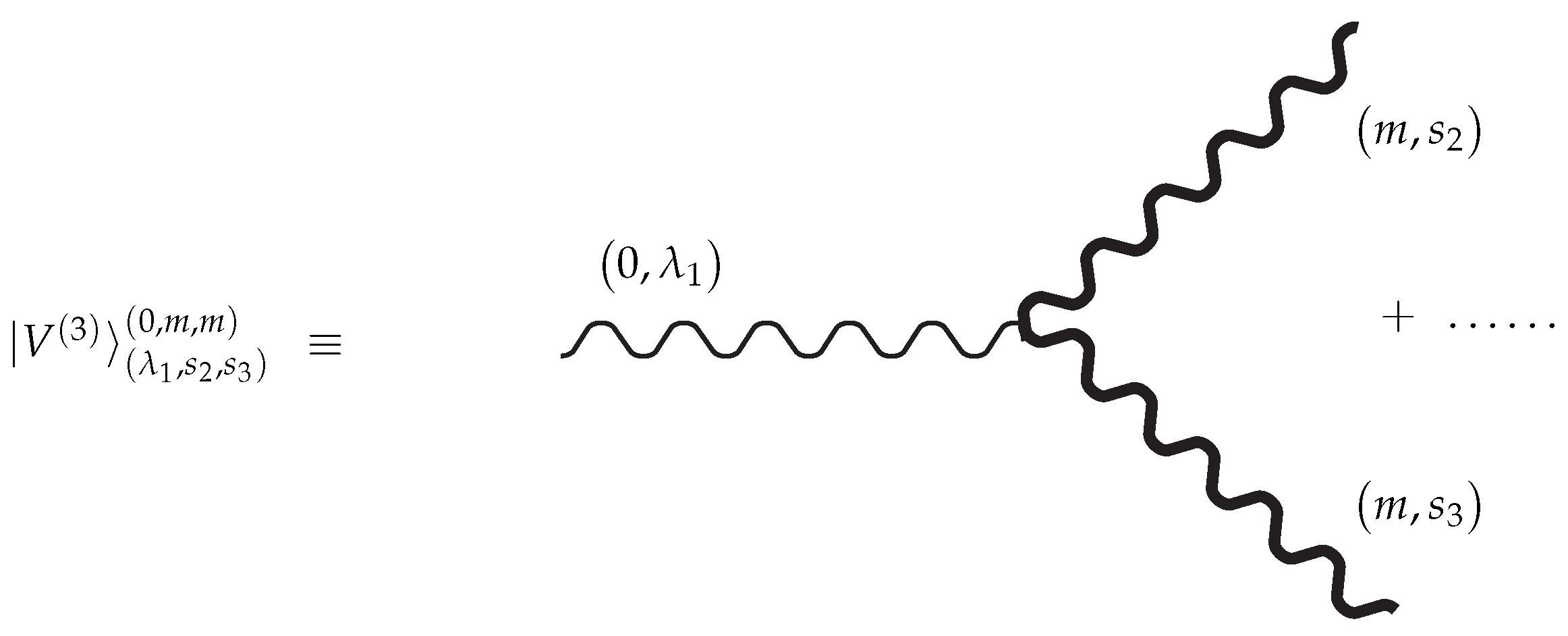
As a result, the solution for the parity invariant vertex (given by Figure 1), has the form

$$\begin{array}{ccc}\hfill |V{}^{\left(3\right)}{\rangle }_{{\left(s\right)}_3}^m& =& |V{}^{M\left(3\right)}{\rangle }_{{\left(s\right)}_3}^m+\sum _{(j_1,j_2,j_3)>0}^{([s_1/2],[s_2/2],[s_3/2])}{U}_{j_3}^{\left(s_1\right)}{U}_{j_3}^{\left(s_2\right)}{U}_{j_3}^{\left(s_3\right)}{|V{}^{M\left(3\right)}\rangle }_{{\left(s\right)}_3-2{\left(j\right)}_3}^m,\hfill \end{array}$$

(78)

where the vertex $|V{}^{M\left(3\right)}{\rangle }_{{\left(s\right)}_3-2{\left(j\right)}_3}^m$ was defined in Metsaev’s paper [18] with account for (28) but with modified forms ${\mathcal{L}}_k^{\left(3\right)}$, (62) and ${\mathcal{L}}_{11|{\sigma }^{(i+2)}}^{(ii+1)+}$ instead of ${\left(L_{11}^{(ii+1)+}\right)}^{{\sigma }^{(i+2)}}$ (46)–(48)

$$\begin{array}{ccc}\hfill V{}_{{\left(s\right)}_3-2{\left(j\right)}_3}^{M\left(3\right)|m}& =& \sum _k{\mathcal{L}}_k^{\left(3\right)}\prod _{i=1}^3{\mathcal{L}}_{11|{\sigma }_{i+2}}^{(ii+1)+},(s,J)=\sum _i\left(s_i,j_i\right),\hfill \end{array}$$

(79)

and is $(3+1)$-parameters family to be enumerated by the natural parameters ${\left(j\right)}_3$, and k subject to the relations

$$\begin{array}{ccc}& & {\sigma }_i=\frac{1}{2}(s-2J-k)-s_i,i=1,2;{\sigma }_3=\frac{1}{2}(s+k)-s_3,\hfill \end{array}$$

(80)

$$\begin{array}{ccc}& & max(0,(s_3-2j_3)-\sum _{i=1}^2(s_i-2j_i))\le k\le s_3-2j_3-|s_1-2j_1-(s_2-2j_2)|,\hfill \end{array}$$

(81)

$$\begin{array}{ccc}& & 0\le 2j_i\le 2[s_i/2],s-2J-k=2p,p\in {\mathbb{N}}_0.\hfill \end{array}$$

(82)

Note, that the vertex in the unconstrained formulation depends on 3 additional parameters ${\left(j\right)}_3$ enumerated the number of traces in the respective set of fields and usual one k respecting the minimal order of derivatives in $V{}_{{\left(s\right)}_3-2{\left(j\right)}_3}^{M\left(3\right)|m}$. For vanishing ${\left(j\right)}_3$, the remaining parameters correspond to one in the constrained BRST formulation [18].

Trace-Deformed Vertex Generalization

The standard trace restriction $\widehat{L}{}_{11}^{\left(i\right)}|{\chi }^{\left(i\right)}\rangle =\widehat{L}{}_{11}^{\left(i\right)}|{\mathrm{\Lambda }}^{\left(i\right)}\rangle =0$ imposed off-shell in constrained BRST approach may be deformed (in the scheme with complete BRST operator) on the interacting level when deriving from resolution of deformed equations of motion and gauge transformations by following $Q^{tot}$-closed modification of the ${\mathcal{L}}_k^{\left(3\right)}$ as compared to (58)–(62)

$$\begin{array}{ccc}\hfill & & {\mathcal{L}}_1^{\left(3\right)}=L^{\left(3\right)}-[\widehat{L}{}_{11}^{\left(3\right)},L^{\left(3\right)}\}\frac{b^{\left(3\right)+}}{h^{\left(3\right)}},\hfill \end{array}$$

(83)

$$\begin{array}{ccc}\hfill & & \tilde{\mathcal{L}}{}_2^{\left(3\right)}={\left({\mathcal{L}}^{\left(3\right)}\right)}^2-i\widehat{\mathcal{P}}{}_0^{\left(3\right)}{\eta }_{11}^{\left(3\right)+}-\widehat{l}{}_0^{\left(3\right)}\frac{b^{\left(3\right)+}}{h^{\left(3\right)}},\hfill \end{array}$$

(84)

$$\begin{array}{ccc}\hfill & & \tilde{\mathcal{L}}{}_{2k}^{\left(3\right)}={\left({\tilde{\mathcal{L}}}_2^{\left(3\right)}\right)}^k,\tilde{\mathcal{L}}{}_{2k-1}^{\left(3\right)}={\left({\tilde{\mathcal{L}}}_2^{\left(3\right)}\right)}^{k-1}{\mathcal{L}}_1^{\left(3\right)},\hfill \end{array}$$

(85)

Note, the representation (83)–(85) contains the term linear in ${\eta }_{11}^{\left(3\right)+}$ without ${\mathcal{P}}_{11}^{\left(3\right)+}$. Thus, the other (more general) solution for the vertex $|V{}^{\left(3\right)}{\rangle }_{{\left(s\right)}_3}^m$ (78) is obtained after the substitution of new $\tilde{\mathcal{L}}{}_k^{\left(3\right)}$ instead of old ones ${\mathcal{L}}_k^{\left(3\right)}$. It is used in Section 5.1.2 for the example with the vertex $|V{}^{\left(3\right)}{\rangle }_{(1,0,s)}^m$ of interacting massive field of spin s with massless scalar and vector fields.

4.2. Cubic Vertices for One Massless Field and Two Massive Fields

In this section, we consider the cases of coinciding and different masses for massive fields

4.2.1. One Massless and Two Massive Fields with Coinciding Masses

In the case (33) with $D=0$, $P_{ϵm}=0$ of massive fields of the same masses $m_2=m_3=m\ne 0$ (critical case) there are the following $Q_c^{tot}$ BRST-closed operators (in minimal derivative scheme)

$$\begin{array}{ccc}\hfill & & \check{L}{}^{\left(i\right)}=\widehat{p}{}_{\mu }^{\left(i\right)}{a}^{\left(i\right)\mu +}+{(-1)}^{i}m{d}^{\left(i\right)+}{\theta }_{i,1}-ı{\widehat{\mathcal{P}}}_0^{\left(i\right)}{\eta }_1^{\left(i\right)+},i=1,2,3\hfill \end{array}$$

(86)

$$\begin{array}{ccc}& & L_{11}^{\left(23\right)+}=a^{\left(2\right)\mu +}{a}_{\mu }^{\left(3\right)+}+\frac{1}{2m}(d^{\left(2\right)+}{L}^{\left(3\right)}-d^{\left(3\right)+}{L}^{\left(2\right)})+d^{\left(2\right)+}{d}^{\left(3\right)+}\hfill \\ & & \phantom{L_{11}^{\left(23\right)+}=}-\frac{1}{2}{\mathcal{P}}_1^{\left(2\right)+}{\eta }_1^{\left(3\right)+}-\frac{1}{2}{\mathcal{P}}_1^{\left(3\right)+}{\eta }_1^{\left(2\right)+},\hfill \end{array}$$

(87)

$$\begin{array}{ccc}& & Z={\tilde{L}}_{11}^{\left(12\right)+}{\check{L}}^{\left(3\right)}+cycl.perm.(1,2,3).\hfill \end{array}$$

(88)

$$\begin{array}{ccc}& & {\tilde{L}}_{11}^{\left(23\right)+}=L_{11}^{\left(23\right)+}-\frac{1}{2m}\left(d^{2)+}{\check{L}}^{\left(3\right)}\right)-d^{3)+}{\check{L}}^{\left(2\right)})\hfill \end{array}$$

(89)

$$\begin{array}{ccc}& & {\tilde{L}}_{11}^{(ii+1)+}=a^{\left(i\right)\mu +}{a}_{\mu }^{(i+1)+}-\frac{1}{2}{\mathcal{P}}_1^{\left(i\right)+}{\eta }_1^{(i+1)+}-\frac{1}{2}{\mathcal{P}}_1^{(i+1)+}{\eta }_1^{\left(i\right)+},i=1,3.\hfill \end{array}$$

(90)

The trace operators $\widehat{L}{}_{11}^{\left(i\right)+}$, $\widehat{L}{}_{11}^{\left(i\right)}$ look for massless field

$$\begin{array}{ccc}& & \left(\widehat{L}{}_{11}^{\left(1\right)+},\widehat{L}{}_{11}^{\left(1\right)}\right)=\left(l_{11}^{\left(1\right)+}+b^{\left(1\right)+}+{\mathcal{P}}_1^{\left(1\right)+}{\eta }_1^{\left(1\right)+},l_{11}^{\left(1\right)}+(b^{\left(1\right)+}{b}^{\left(1\right)}+h^{\left(1\right)})b^{\left(1\right)}+{\eta }_1^{\left(1\right)}{\mathcal{P}}_1^{\left(1\right)}\right)\hfill \end{array}$$

(91)

and according to (6) and (7) for massive case when $i=2,3$

$$\begin{array}{ccc}& & \widehat{L}{}_{11}^{\left(i\right)+}=l_{11}^{\left(i\right)+}-(1/2){\left(d^{\left(i\right)+}\right)}^2+b^{\left(i\right)+}+{\mathcal{P}}_1^{\left(i\right)+}{\eta }_1^{\left(i\right)+},\hfill \end{array}$$

(92)

$$\begin{array}{ccc}& & \widehat{L}{}_{11}^{\left(i\right)}=l_{11}^{\left(i\right)}-(1/2){\left(d^{\left(i\right)}\right)}^2+(b^{\left(i\right)+}{b}^{\left(i\right)}+h^{\left(i\right)})b^{\left(i\right)}+{\eta }_1^{\left(i\right)}{\mathcal{P}}_1^{\left(i\right)}.\hfill \end{array}$$

(93)

The general solution for the parity invariant cubic vertex describing interaction for irreducible massless field with helicity $s_1$ and two massive with spins $s_2$, $s_3$ with the same masses ${\left(\overline{m}\right)}_2=(0,m,m)$ is shown in Figure 2, and has the form

$$\begin{array}{ccc}\hfill |V{}^{\left(3\right)}{\rangle }_{{\left(s\right)}_3}^{{\left(\overline{m}\right)}_2}& =& |V{}^{M\left(3\right)}{\rangle }_{{\left(s\right)}_3}^{{\left(\overline{m}\right)}_2}+\sum _{(j_3,j_3,j_3)>0}^{([s_1/2],[s_2/2],[s_3/2])}{U}_{j_3}^{\left(s_1\right)}{U}_{j_3}^{\left(s_2\right)}{U}_{j_3}^{\left(s_3\right)}{|V{}^{M\left(3\right)}\rangle }_{{\left(s\right)}_3-2{\left(j\right)}_3}^{{\left(\overline{m}\right)}_2},\hfill \end{array}$$

(94)

where the vertex $|V{}^{M\left(3\right)}{\rangle }_{{\left(s\right)}_3-2{\left(j\right)}_3}^{{\left(\overline{m}\right)}_2}$ was defined in Metsaev’s paper [18] for ${\left(j\right)}_3=0$ with account for (86)–(90) but with modified forms ${\check{\mathcal{L}}}_{k_i}^{\left(i\right)}$,

$$\begin{array}{ccc}& & {\check{\mathcal{L}}}_{k_i}^{\left(i\right)}=\sum _{j=0}^{[k_i/2]}{(-1)}^j{\left({\check{L}}^{\left(i\right)}\right)}^{k_i-2j}{\left({\widehat{p}}^{\left(i\right)}\right)}^{2j}\frac{k_i!}{j!2^j(k_i-2j))!}\frac{{\left(b^{\left(i\right)+}\right)}^j}{C(j,h^{\left(i\right)})},\hfill \\ & & \mathrm{for}{\left({\widehat{p}}^{\left(i\right)}\right)}^2={\eta }^{\mu \nu }(p_{\mu }^{(i+1)}-p_{\mu }^{(i+2)})(p_{\nu }^{(i+1)}-p_{\nu }^{(i+2)})-{(-1)}^i{m}^2{\theta }_{i,1},i=1,2,3.\hfill \end{array}$$

(95)

and forms ${\mathcal{L}}_{11|{\sigma }_{(i+2)}}^{(ii+1)+}$ instead of polynomials ${\left(L_{11}^{(ii+1)+}\right)}^{{\sigma }_{(i+2)}}$ given in (89), (90) for $i=1,2,3$:

$$\begin{array}{ccc}\hfill & & {\mathcal{L}}_{11|1}^{(ii+1)+}=L_{11}^{(ii+1)+}-\sum _{i_0=i}^{i+1}{W}_{(ii+1)|0}^{\left(i_0\right)}\frac{b^{\left(i_0\right)+}}{h^{\left(i_0\right)}}+\frac{1}{2}(\sum _{i_0\ne j_0}[\widehat{L}{}_{11}^{\left(j_0\right)},W_{(ii+1)|0}^{\left(i_0\right)}\}\frac{b^{\left(i_0\right)+}}{h^{\left(i_0\right)}}\frac{b^{\left(j_0\right)+}}{h^{\left(j_0\right)}}\hfill \\ & & +\sum _{i_0}[\widehat{L}{}_{11}^{\left(i_0\right)},W_{(ii+1)|0}^{\left(i_0\right)}\}\frac{{\left(b^{\left(i_0\right)+}\right)}^2}{h^{\left(i_0\right)}(h^{\left(i_0\right)}+1)}),\hfill \end{array}$$

(96)

$$\begin{array}{ccc}& & {\mathcal{L}}_{11|k+1}^{(ii+1)+}=L_{11}^{(ii+1)+}{\mathcal{L}}_{11|k}^{(ii+1)+}-\sum _{i_k=i}^{i+1}{W}_{(ii+1)|k}^{\left(i_k\right)}\frac{b^{\left(i_k\right)+}}{h^{\left(i_k\right)}}+\frac{1}{2}(\sum _{i_k\ne j_k}[\widehat{L}{}_{11}^{\left(j_k\right)},W_{(ii+1)|k}^{\left(i_k\right)}\}\hfill \\ & & \times \frac{b^{\left(i_k\right)+}}{h^{\left(j_k\right)}}\frac{b^{\left(j_k\right)+}}{h^{\left(j_k\right)}}+\sum _{i_k}[\widehat{L}{}_{11}^{\left(i_k\right)},W_{(ii+1)|k}^{\left(i_k\right)}\}\frac{{\left(b^{\left(i_k\right)+}\right)}^2}{{\prod }_{p=0}^1(h^{\left(i_k\right)}+p)})+\sum _{e=3}^{k+2}\frac{{(-1)}^e}{e!}\times \hfill \\ & & \times \sum _{l=0,j\ne i}^{[e/2]}\frac{e!}{[e/(e-l\left)\right](e-l)!l!}{\mathrm{ad}}_{\widehat{L}{}_{11}^{\left(j_k\right)}}^l{\mathrm{ad}}_{\widehat{L}{}_{11}^{\left(i_k\right)}}^{e-l-1}{W}_{(ii+1)|k}^{\left(i_k\right)}\frac{{\left(b^{\left(j_k\right)+}\right)}^l}{C(l,h^{\left(j_k\right)})}\frac{{\left(b^{\left(i_k\right)+}\right)}^{e-l}}{C(e-l,h^{\left(i_k\right)})}.\hfill \end{array}$$

(97)

(for $k=1,\dots ,min(s_i,s_{i+1})-1$) and with $Q^{tot}$- BRST-closed polynomials ${\mathcal{Z}}^{\lambda }$, for $\lambda =1,2,\dots ,min(s_1,s_2,s_3)$ constructed from BRST-closed forms ${\tilde{\mathcal{L}}}_{11|1}^{(ii+1)+}$ according to (96), subject to change of ${\mathcal{L}}_{11|1}^{(ii+1)+}$ on one with tilde and ${\tilde{\mathcal{L}}}_1^{\left(i\right)}$:

$$\begin{array}{ccc}& & \mathcal{Z}={\tilde{\mathcal{L}}}_{11|1}^{\left(12\right)+}{\check{\mathcal{L}}}_1^{\left(3\right)}+cycl.perm.(1,2,3).\mathrm{with}{\tilde{\mathcal{L}}}_1^{\left(i\right)}=\check{L}{}^{\left(i\right)}-[\widehat{L}{}_{11}^{\left(i\right)},{\check{L}}^{\left(i\right)}\}\frac{b^{\left(3\right)+}}{h^{\left(3\right)}}.\hfill \end{array}$$

(98)

Explicitly, the vertex $V{}_{{\left(s\right)}_3-2{\left(j\right)}_3}^{M\left(3\right)|{\left(\overline{m}\right)}_2}$ is determined by

$$\begin{array}{ccc}\hfill V{}_{{\left(s\right)}_3-2{\left(j\right)}_3}^{M\left(3\right)|{\left(\overline{m}\right)}_2}& =& \sum _{\sigma ,\lambda }{\mathcal{L}}_{11|\sigma }^{\left(23\right)+}{\mathcal{Z}}^{\lambda }\prod _{i=1}^3{\check{\mathcal{L}}}_{k_i}^{\left(i\right)},\mathrm{for}0\le k_1\le s_1-2j_1\hfill \end{array}$$

(99)

and is $(3+2)$-parameter family to be enumerated by the natural parameters (corresponding for traces) ${\left(j\right)}_3$, and $k_{min}$, $k_{max}$ (corresponding for order of derivatives) subject to the equations

$$\begin{array}{ccc}& & k_1=k_{min},k_2=k_{max}-k_{min}-(s_3-2j_3),k_3=k_{max}-k_{min}-(s_3-2j_3),\hfill \end{array}$$

(100)

$$\begin{array}{ccc}& & \sigma =s-2(s_1-2j_1)-k_{max}+2k_{min},\lambda =s_1-2j_1-k_{min},\hfill \\ & & \left[max(s_2-2j_2,s_3-2j_3)\right]\le k_{max}-k_{min}\le \left[s-2(s_1-2j_1)+k_{min}\right].\hfill \end{array}$$

(101)

The representation for the vertex (94) and (99) for irreducible massless and massive fields with the same masses presents the basic results of this subsection. For vanishing ${\left(j\right)}_3$ remaining parameters correspond to ones in constrained BRST formulation [18].

4.2.2. One Massless Field and Two Massive Fields with Different Masses

For the case (34) with $D>0$ with different non-vanishing masses $m_3\ne m_2$ we start from $Q_c^{tot}$ BRST-closed operators, with except for $L^{\left(1\right)}$ (in minimal derivative scheme)

$$\begin{array}{ccc}\hfill & & L^{\left(i\right)}=\widehat{p}{}_{\mu }^{\left(i\right)}{a}^{\left(i\right)\mu +}+{(-1)}^i\frac{{\delta }_{i2}{m}_3^2+{\delta }_{i3}{m}_2^2}{m_i}{d}^{\left(i\right)+}-ı\widehat{\mathcal{P}}{}_0^{\left(i\right)}{\eta }_1^{\left(i\right)+},i=1,2,3;\hfill \end{array}$$

(102)

$$\begin{array}{ccc}& & L_{11}^{\left(23\right)+}=a^{\left(2\right)\mu +}{a}_{\mu }^{\left(3\right)+}+\frac{d^{\left(2\right)+}}{2m_2}{L}^{\left(3\right)}-\frac{d^{\left(3\right)+}}{2m_3}{L}^{\left(2\right)}+\frac{m_2^2+m_3^2}{2m_2{m}_3}{d}^{\left(2\right)+}{d}^{\left(3\right)+}\hfill \\ & & \phantom{L_{11}^{\left(23\right)+}}-\frac{1}{2}{\mathcal{P}}_1^{\left(2\right)+}{\eta }_1^{\left(3\right)+}-\frac{1}{2}{\mathcal{P}}_1^{\left(3\right)+}{\eta }_1^{\left(2\right)+},\hfill \end{array}$$

(103)

$$\begin{array}{ccc}& & L_{11}^{\left(12\right)+}=a^{\left(1\right)\mu +}{a}_{\mu }^{\left(2\right)+}-\left(\frac{d^{\left(2\right)+}}{2m_2}+\frac{L^{\left(2\right)}}{2(m_3^2-m_2^2)}\right)L^{\left(1\right)}-\frac{1}{2}{\mathcal{P}}_1^{\left(1\right)+}{\eta }_1^{\left(2\right)+}-\frac{1}{2}{\mathcal{P}}_1^{\left(2\right)+}{\eta }_1^{\left(1\right)+},\hfill \end{array}$$

(104)

$$\begin{array}{ccc}& & L_{11}^{\left(31\right)+}=a^{\left(3\right)\mu +}{a}_{\mu }^{\left(1\right)+}+\left(\frac{d^{\left(3\right)+}}{2m_3}+\frac{L^{\left(3\right)}}{2(m_3^2-m_2^2)}\right)L^{\left(1\right)}-\frac{1}{2}{\mathcal{P}}_1^{\left(3\right)+}{\eta }_1^{\left(1\right)+}-\frac{1}{2}{\mathcal{P}}_1^{\left(1\right)+}{\eta }_1^{\left(3\right)+},\hfill \end{array}$$

(105)

The general solution for the parity invariant cubic vertex describing interaction for irreducible massless field with helicity $s_1$ and two massives with spins $s_2$, $s_3$ with different masses is shown by Figure 3 and has the representation in terms of the product of BRST-closed (with respective complete BRST operator $Q^{tot}$ in question) forms

$$\begin{array}{ccc}\hfill |V{}^{\left(3\right)}{\rangle }_{{\left(s\right)}_3}^{{\left(m\right)}_2}& =& |V{}^{M\left(3\right)}{\rangle }_{{\left(s\right)}_3}^{{\left(m\right)}_2}+\sum _{(j_3,j_3,j_3)>0}^{([s_1/2],[s_2/2],[s_3/2])}{U}_{j_3}^{\left(s_1\right)}{U}_{j_3}^{\left(s_2\right)}{U}_{j_3}^{\left(s_3\right)}{|V{}^{M\left(3\right)}\rangle }_{{\left(s\right)}_3-2{\left(j\right)}_3}^{{\left(m\right)}_2},\hfill \end{array}$$

(106)

where the vertex $|V{}^{M\left(3\right)}{\rangle }_{{\left(s\right)}_3-2{\left(j\right)}_3}^{{\left(m\right)}_2}$ was given in [18] with account for (102)–(105) but with modified forms ${\mathcal{L}}_{k_i}^{\left(i\right)}$, (108) and ${\mathcal{L}}_{11|{\sigma }_{(j+2)}}^{(jj+1)+}$ (110), (77) instead of ${\left(L_{11}^{(jj+1)+}\right)}^{{\sigma }_{(j+2)}}$

$$\begin{array}{ccc}\hfill V{}_{{\left(s\right)}_3-2{\left(j\right)}_3}^{M\left(3\right)|{\left(m\right)}_2}& =& \sum _{{\tau }_2,{\tau }_3}\prod _{i=2}^3{\mathcal{L}}_{{\tau }_i}^{\left(i\right)}\prod _{r=1}^3{\mathcal{L}}_{11|{\sigma }_{r+2}}^{(rr+1)+},\hfill \end{array}$$

(107)

were the ranges for ${\tau }_2,{\tau }_3,{\sigma }_1,{\sigma }_2,{\sigma }_3$ are specified below. Here,

$$\begin{array}{ccc}& & {\mathcal{L}}_{k_i}^{\left(i\right)}=\sum _{j=0}^{[k_i/2]}{(-1)}^j{\left(L^{\left(i\right)}\right)}^{k_i-2j}{\left({\widehat{p}}^{\left(i\right)}\right)}^{2j}\frac{k_i!}{j!2^j(k_i-2j))!}\frac{{\left(b^{\left(i\right)+}\right)}^j}{C(j,h^{\left(i\right)})},\hfill \end{array}$$

(108)

$$\begin{array}{ccc}& & \mathrm{for}{\left({\widehat{p}}^{\left(i\right)}\right)}^2={\eta }^{\mu \nu }(p_{\mu }^{(i+1)}-p_{\mu }^{(i+2)})(p_{\nu }^{(i+1)}-p_{\nu }^{(i+2)})-\frac{{({\delta }_{i2}{m}_3^2+{\delta }_{i3}{m}_2^2)}^2}{m_i^2},i=2,3.\hfill \end{array}$$

(109)

and for mixed trace operators, when $i=1,2,3$

$$\begin{array}{ccc}\hfill & & {\mathcal{L}}_{11|1}^{(ii+1)+}=L_{11}^{(ii+1)+}-\sum _{i_0=i}^{i+1}{W}_{(ii+1)|0}^{\left(i_0\right)}\frac{b^{\left(i_0\right)+}}{h^{\left(i_0\right)}}+\frac{1}{2}(\sum _{i_0\ne j_0}[\widehat{L}{}_{11}^{\left(j_0\right)},W_{(ii+1)|0}^{\left(i_0\right)}\}\frac{b^{\left(i_0\right)+}}{h^{\left(i_0\right)}}\frac{b^{\left(j_0\right)+}}{h^{\left(j_0\right)}}\hfill \\ & & +\sum _{i_0}[\widehat{L}{}_{11}^{\left(i_0\right)},W_{(ii+1)|0}^{\left(i_0\right)}\}\frac{{\left(b^{\left(i_0\right)+}\right)}^2}{h^{\left(i_0\right)}(h^{\left(i_0\right)}+1)}),\hfill \end{array}$$

(110)

$$\begin{array}{ccc}& & {\mathcal{L}}_{11|k+1}^{(ii+1)+}=L_{11}^{(ii+1)+}{\mathcal{L}}_{11|k}^{(ii+1)+}-\sum _{i_k=i}^{i+1}{W}_{(ii+1)|k}^{\left(i_k\right)}\frac{b^{\left(i_k\right)+}}{h^{\left(i_k\right)}}+\frac{1}{2}(\sum _{i_k\ne j_k}[\widehat{L}{}_{11}^{\left(j_k\right)},W_{(ii+1)|k}^{\left(i_k\right)}\}\hfill \\ & & \times \frac{b^{\left(i_k\right)+}}{h^{\left(j_k\right)}}\frac{b^{\left(j_k\right)+}}{h^{\left(j_k\right)}}+\sum _{i_k}[\widehat{L}{}_{11}^{\left(i_k\right)},W_{(ii+1)|k}^{\left(i_k\right)}\}\frac{{\left(b^{\left(i_k\right)+}\right)}^2}{{\prod }_{p=0}^1(h^{\left(i_k\right)}+p)})+\sum _{e=3}^{k+2}\frac{{(-1)}^e}{e!}\times \hfill \\ & & \times \sum _{l=0,j\ne i}^{[e/2]}\frac{e!}{[e/(e-l\left)\right](e-l)!l!}{\mathrm{ad}}_{\widehat{L}{}_{11}^{\left(j_k\right)}}^l{\mathrm{ad}}_{\widehat{L}{}_{11}^{\left(i_k\right)}}^{e-l-1}{W}_{(ii+1)|k}^{\left(i_k\right)}\frac{{\left(b^{\left(j_k\right)+}\right)}^l}{C(l,h^{\left(j_k\right)})}\frac{{\left(b^{\left(i_k\right)+}\right)}^{e-l}}{C(e-l,h^{\left(i_k\right)})}\hfill \end{array}$$

(111)

(for $k=1,\dots ,min(s_i,s_{i+1})-1$). The vertex (107) represents the $(3+2)$-parameter family to be enumerated by the natural parameters ${\left(j\right)}_3$, and ${\tau }_2,{\tau }_3$ subject to the equations

$$\begin{array}{ccc}& & {\sigma }_i=\frac{1}{2}[s-2J-2(s_i-2j_i)-{(-1)}^{{\delta }_{i1}}{\tau }_2-{(-1)}^{{\delta }_{i2}}{\tau }_3],i=1,2,3;\hfill \end{array}$$

(112)

$$\begin{array}{ccc}& & |\sum _{i=2}^3{(-1)}^i(s_i-2j_i-{\tau }_i)|\le s_1-2j_1\le \sum _{i=2}^3(s_i-2j_i-{\tau }_i),\hfill \end{array}$$

(113)

$$\begin{array}{ccc}& & s-2J-{\tau }_2-{\tau }_3=2p,p\in {\mathbb{N}}_0.\hfill \end{array}$$

(114)

The relations for the vertex (106) and (107) for irreducible massless and massive fields with different masses present our basic results in the subsection. Again, for vanishing ${\left(j\right)}_3$ the remaining parameters correspond to the ones in the constrained BRST formulation [18].

5. Examples for HS Fields with Special Spin Values

Here, we consider ghost-independent and component (tensor) forms of the cubic vertices for special cases of interacting higher spin fields.

5.1. Vertices for Fields with $(m,s)$, $(0,{\lambda }_1)$, $(0,{\lambda }_2)$

In the subsection, we derive the cubic vertices $V{}_{{\left(s\right)}_3}^{M\left(3\right)|m}$ for one massive HS field with $(m,s)$ and two massless HS fields with $(0,{\lambda }_1)$, $(0,{\lambda }_2)$ with small values of two spin parameters.

5.1.1. Case $(m,s)$, $(0,{\lambda }_i)$ for ${\lambda }_i=0$

First, for the interaction of 2 massless scalars with a massive HS field we have, according to (78) and (79), the j-parameter family of vertices for $j=1,\dots ,[s/2]$ restoring the dimensional coupling constants $t_j$ ($dim{t}_j$=$s+d/2-3-2j$, in metric units providing a dimensionless of the action)

$$\begin{array}{ccc}\hfill V{}_{(0,0,s)}^{\left(3\right)|m}& =& \sum _{j\ge 0}^{[s/2]}{t}_j{U}_j^{\left(s\right)}{\mathcal{L}}_{s-2j}^{\left(3\right)}=\sum _{j\ge 0}^{[s/2]}{t}_j{U}_j^{\left(s\right)}\sum _{i=0}^{\left[\right(s-2j)/2]}{(-1)}^i{\left(L^{\left(3\right)}\right)}^{s-2j-2i}\times \hfill \\ & & \times {\left({\widehat{p}}^{\left(3\right)}\right)}^{2i}\frac{(s-2j)!}{i!2^i(s-2j-2i)!}\frac{{\left(b^{\left(3\right)+}\right)}^i}{C(i,h^{\left(3\right)})},\hfill \end{array}$$

(115)

with following decomposition in powers of ${\eta }_1^{\left(3\right)+}$ for the operators

$$\begin{array}{ccc}\hfill & & {\left(L^{\left(3\right)}\right)}^k={\left(L^{\left(3\right)}\right)}_0^k-ık{\widehat{\mathcal{P}}}_0^{\left(3\right)}{\eta }_1^{\left(3\right)+}{\left(L^{\left(3\right)}\right)}_0^{k-1}\equiv {\left(\widehat{p}{}_{\mu }^{\left(3\right)}{a}^{\left(i\right)\mu +}\right)}^{k-1}\left(\widehat{p}{}_{\mu }^{\left(3\right)}{a}^{\left(3\right)\mu +}-ık{\widehat{\mathcal{P}}}_0^{\left(3\right)}{\eta }_1^{\left(3\right)+}\right),\hfill \end{array}$$

(116)

$$\begin{array}{ccc}\hfill & & {\mathcal{L}}_k^{\left(3\right)}={\mathcal{L}}_k^{\left(3\right)0}-ı{\widehat{\mathcal{P}}}_0^{\left(3\right)}{\eta }_1^{\left(3\right)+}{\left({\mathcal{L}}_{k-1}^{\left(3\right)}\right)}^{\prime }\equiv {\mathcal{L}}_k^{\left(3\right)}{|}_{{\eta }_1^{\left(3\right)+}=0}\hfill \\ & & -ı{\widehat{\mathcal{P}}}_0^{\left(3\right)}{\eta }_1^{\left(3\right)+}\sum _{i=0}^{[k/2]}{(-1)}^i{\left(L^{\left(3\right)}\right)}_0^{k-1-2i}{\left({\widehat{p}}^{\left(3\right)}\right)}^{2i}\frac{k!}{i!2^i(k-1-2i)!}\frac{{\left(b^{\left(3\right)+}\right)}^i}{C(i,h^{\left(3\right)})}.\hfill \end{array}$$

(117)

The interacting part of the action $S_{{\left[1\right]|\left(s\right)}_3}^{{\left(m\right)}_3}$ (21) for ${\left(m\right)}_3=(0,0,m)$, ${\left(s\right)}_3=(0,0,s)$ depends only on basic $\mathbb{R}$-valued fields ${\varphi }^{\left(1\right)}$, ${\varphi }^{\left(2\right)}$${\varphi }_{\mu \left(s\right)}^{\left(3\right)}$ and on auxiliary ones $|{\varphi }_{\mu (s-k-2l)|k,l}^{\left(3\right)}$. for $k=0,\dots ,s$; $l=0,\dots ,[s-k/2]$, ($k+l>0$) according to (19):

$$S_{{1|\left(s\right)}_3}^{{\left(m\right)}_3}[{\varphi }^{\left(1\right)},{\varphi }^{\left(2\right)},{\chi }^{\left(3\right)}]=g\int \prod _{i=1}^{3}d{\eta }_0^{\left(i\right)}\left({}_s\langle {\chi }^{\left(3\right)}{K}^{\left(3\right)}|{}_0\langle {\varphi }^{\left(2\right)}|{}_0{\langle {\varphi }^{\left(1\right)}|V{}^{\left(3\right)}\rangle }_{{\left(s\right)}_3}^m+h.c.\right),$$

(118)

whereas the ghost-independent form for initial free action looks like

$$\begin{array}{ccc}\hfill & & \sum _{i=1}^3{\mathcal{S}}_{0|s_i}^{m_i}=\int d^{d}x\left[\sum _{i=1}^2{\varphi }^{\left(i\right)}\square {\varphi }^{\left(i\right)}+{\mathcal{S}}_{0|s}^m\left[{\chi }^{\left(3\right)}\right]\right],\hfill \end{array}$$

(119)

where the functional ${\mathcal{S}}_{0|s}^m\left[{\chi }^{\left(3\right)}\right]$ is explicitly determined in (A1), (A2) and invariant with respect to the initial gauge transformations for the field $|{\chi }^{\left(3\right)}{\rangle }_s$ (A3)–(A12) and for the gauge parameter $|{\mathrm{\Lambda }}^{\left(3\right)}{\rangle }_s$ (A13). The gauge symmetry is untouched under the deformation for the interacting massive field $|{\mathrm{\Phi }}_{\dots }^{\left(3\right)}{\rangle }_{s-\dots }$, whereas in the sector of scalar fields they admit non-linear deformation

$$\begin{array}{ccc}& & {\delta }_{\left[1\right]}\left(|{\chi }^{\left(3\right)}{{\rangle }_s,|{\mathrm{\Lambda }}^{\left(3\right)}\rangle }_s\right)=Q^{\left(3\right)}\left(|{\mathrm{\Lambda }}^{\left(3\right)}{{\rangle }_s,|{\mathrm{\Lambda }}^{\left(3\right)1}\rangle }_s\right),\hfill \end{array}$$

(120)

$$\begin{array}{ccc}& & {\delta }_{\left[1\right]}|{\varphi }^{\left(1\right)}{\rangle }_0=-g\int d{\eta }_0^{\left(2\right)}d{\eta }_0^{\left(3\right)}{}_s\langle {\mathrm{\Lambda }}^{\left(3\right)}{K}^{\left(3\right)}|{}_0{\langle {\varphi }^{\left(2\right)}|V{}^{\left(3\right)}\rangle }_{{\left(s\right)}_3}^m,\hfill \end{array}$$

(121)

$$\begin{array}{ccc}& & {\delta }_{\left[1\right]}|{\varphi }^{\left(2\right)}{\rangle }_0=-g\int d{\eta }_0^{\left(3\right)}d{\eta }_0^{\left(1\right)}({}_s\langle {\mathrm{\Lambda }}^{\left(3\right)}{K}^{\left(3\right)}|{}_0{\langle {\varphi }^{\left(1\right)}|V{}^{\left(3\right)}\rangle }_{{\left(s\right)}_3}^m.\hfill \end{array}$$

(122)

The values of parameters $h^{\left(i\right)}\left(s_i\right)$ are equal to $h^{\left(1\right)}\left(0\right)=h^{\left(2\right)}\left(0\right)=-(d-6)/2$ and $h^{\left(3\right)}\left(s\right)=-s-(d-5)/2$.

The interacting part of action $S_{{1|\left(s\right)}_3}^{{\left(m\right)}_3}$ (118) is written in the ghost-independent form

$$\begin{array}{ccc}\hfill & & S_{{1|\left(s\right)}_3}^{{\left(m\right)}_3}[{\varphi }^{\left(1\right)},{\varphi }^{\left(2\right)},{\chi }^{\left(3\right)}]=-g\prod _{i=2}^3{\delta }^{\left(d\right)}\left(x_1-x_i\right)\left(\right\{{}_0\langle {\varphi }^{\left(2\right)}|{}_0\langle {\varphi }^{\left(1\right)}\left|\right({}_s\langle {\mathrm{\Phi }}^{\left(3\right)}{K}^{\left(3\right)}|\hfill \\ & & \times \sum _{j\ge 0}^{[s/2]}{t}_j{\left(\check{L}{}_{11}^{\left(3\right)+}\right)}^j{\mathcal{L}}_{s-2j}^{\left(3\right)0}+{}_{s-2}\langle {\mathrm{\Phi }}_2^{\left(3\right)}{K}^{\left(3\right)}|\sum _{j\ge 0}^{[s/2]-1}{t}_j(j+1){\left(\check{L}{}_{11}^{\left(3\right)+}\right)}^j{\mathcal{L}}_{s-2(j+1)}^{\left(3\right)0}\hfill \\ & & +{}_{s-4}\langle {\mathrm{\Phi }}_{32}^{\left(3\right)}{K}^{\left(3\right)}|\sum _{j\ge 0}^{[s/2]-2}{t}_j(j+1)(j+2){\left(\check{L}{}_{11}^{\left(3\right)+}\right)}^j{\mathcal{L}}_{s-2(j+2)}^{\left(3\right)0}\hfill \\ & & -{}_{s-6}\langle {\mathrm{\Phi }}_{22}^{\left(3\right)}{K}^{\left(3\right)}|\sum _{j\ge 0}^{[s/2]-3}{t}_j(j+1)(j+2)(j+3){\left(\check{L}{}_{11}^{\left(3\right)+}\right)}^j{\mathcal{L}}_{s-2(j+3)}^{\left(3\right)0}\}|0\rangle +h.c.),\hfill \end{array}$$

(123)

jointly with the gauge transformation

$$\begin{array}{ccc}& & {\delta }_{\left[1\right]}|{\varphi }^{\left(1\right)}{\rangle }_0=-g\prod _{i=2}^3{\delta }^{\left(d\right)}\left(x_1-x_i\right){}_0\langle {\varphi }^{\left(2\right)}\left|\right\{{}_{s-1}\langle {\mathrm{\Xi }}^{\left(3\right)}{K}^{\left(3\right)}|\sum _{j\ge 0}^{[s-1/2]}{t}_j{\left(\check{L}{}_{11}^{\left(3\right)+}\right)}^j{\left({\mathcal{L}}_{s-1-2j}^{\left(3\right)}\right)}^{\prime }\hfill \\ & & -{}_{s-5}\langle {\mathrm{\Xi }}_{12}^{\left(3\right)}{K}^{\left(3\right)}|\sum _{j\ge 0}^{[s-5/2]}{t}_j(j+1)(j+2){\left(\check{L}{}_{11}^{\left(3\right)+}\right)}^j{\left({\mathcal{L}}_{s-5-2j}^{\left(3\right)}\right)}^{\prime }\}|0\rangle ,\hfill \end{array}$$

(124)

$$\begin{array}{ccc}& & {\delta }_{\left[1\right]}|{\varphi }^{\left(2\right)}{\rangle }_0=-{\delta }_{\left[1\right]}|{\varphi }^{\left(1\right)}{{\rangle }_0|}_{\left({\varphi }^{\left(1\right)}\left(x_1\right)\to {\varphi }^{\left(2\right)}\left(x_2\right)\right)}.\hfill \end{array}$$

(125)

In deriving the action (123) we have taken the vanishing of the term $\widehat{\mathcal{P}}{}_0^{\left(3\right)}$, whereas for the transformations (124) and (125) its necessary presence in $L^{\left(3\right)}$ by the rule (117). In addition, we have used for $U_j^{\left(s\right)}$ the decomposition in powers of ghost oscillators, according to (6) and (54)

$$\begin{array}{ccc}\hfill & & U_j^{\left(s\right)}={\left(\check{L}{}_{11}^{\left(3\right)+}\right)}^{(j-3)}[{\left(\check{L}{}_{11}^{+\left(3\right)}\right)}^3+j{\left(\check{L}{}_{11}^{+\left(3\right)}\right)}^2{\mathcal{P}}_1^{\left(3\right)+}{\eta }_1^{\left(3\right)+}+j(j-1){\mathcal{P}}_{11}^{\left(3\right)+}{\eta }_{11}^{\left(3\right)+}\hfill \\ & & \phantom{U_j^{\left(s\right)}}\times \left[\check{L}{}_{11}^{+\left(3\right)}+\left(j-2\right){\mathcal{P}}_1^{\left(3\right)+}{\eta }_1^{\left(3\right)+}\right\}].\hfill \end{array}$$

(126)

Presenting the above expressions in the oscillator forms, first, for cubic in field action (A23), second, for linear in field generators of the gauge transformations (A24), (A25) and calculating the underlying scalar products by the rules (A26)–(A28) we obtain finally, for the action (A23) with accuracy up to overall factor ${(-1)}^{s}s!$ the representation (A34)

$$\begin{array}{ccc}\hfill & & S_{{1|\left(s\right)}_3}^{{\left(m\right)}_3}=S_1^{\left(0\right)}\left[{\varphi }^{\left(a\right)},{\mathrm{\Phi }}^{\left(3\right)}\right]+S_1^{\left(2\right)}\left[{\varphi }^{\left(a\right)},{\mathrm{\Phi }}_2^{\left(3\right)}\right]+S_1^{\left(32\right)}\left[{\varphi }^{\left(a\right)},{\mathrm{\Phi }}_{32}^{\left(3\right)}\right]+S_1^{\left(22\right)}\left[{\varphi }^{\left(a\right)},{\mathrm{\Phi }}_{22}^{\left(3\right)}\right],\hfill \end{array}$$

(127)

(for ${\varphi }^{\left(a\right)}=({\varphi }^{\left(1\right)},{\varphi }^{\left(2\right)})$) also for the gauge transformations (A24), (A25) given by (A35), (A36)

$$\begin{array}{ccc}\hfill & & {\delta }_{\left[1\right]}{\varphi }^{\left(a\right)}\left(x_a\right)={(-1)}^{a+1}\left({\delta }_{1|{\mathrm{\Xi }}^{\left(3\right)}}{\varphi }^{\left(a\right)}\left(x_a\right)+{\delta }_{1|{\mathrm{\Xi }}_{12}^{\left(3\right)}}{\varphi }^{\left(a\right)}\left(x_a\right)\right),a=1,2.\hfill \end{array}$$

(128)

Let us discuss the obtained solution. The part of vertex $\widehat{S}{}_{{1|\left(s\right)}_3}^{{\left(m\right)}_3}=S_{{1|\left(s\right)}_3}^{{\left(m\right)}_3}{|}_{j=0}$ (127) without traces (for $j=0$, and therefore, for $l=k=0$) with only initial ${\varphi }_{0,0}^{\left(3\right)\nu \left(s\right)}$ and auxiliary ${\varphi }_{i,0}^{\left(3\right)\nu \left(s-2i\right)}$, $i=1,\dots ,[s/2]$ fields reads

$$\begin{array}{ccc}\hfill & & \widehat{S}{}_{{1|\left(s\right)}_3}^{{\left(m\right)}_3}=-2g{t}_0\int d^{d}x[\sum _{i=0}^{[s/2]}\frac{\left(s\right)!}{i!}\sum _{u=0}^{s-2i}\frac{{(-1)}^u}{u!(s-2i-u)!}\sum _{q=0}^i\sum _{t=0}^{i-q}{C}_i^{q,t}\frac{{(-1)}^t}{2^{i-t}}\hfill \\ & & \times \left[{\partial }_{{\nu }_0}\dots {\partial }_{{\nu }_u}\left({\partial }_{{\nu }_{u+1}}\dots {\partial }_{{\nu }_{u+t}}{\square }^q{\varphi }^{\left(1\right)}\right)\right]\left[{\partial }_{{\nu }_{u+t+1}}\dots {\partial }_{{\nu }_{s-2i+t}}{\partial }^{{\nu }_{u+1}}\dots {\partial }^{{\nu }_{u+t}}{\square }^{i-q-t}{\varphi }^{\left(2\right)}\right]{\varphi }_{i,0}^{\left(3\right)\nu \left(s-2i\right)}\}.\hfill \end{array}$$

(129)

The respective gauge transformations ${\widehat{\delta }}_{\left[1\right]}{\varphi }^{\left(1\right)}={\delta }_{\left[1\right]}{\varphi }^{\left(1\right)}{|}_{j=0}$ from (128) depending only on the coupling constant $t_0$ take the form

$$\begin{array}{ccc}\hfill & & {\widehat{\delta }}_{\left[1\right]}{\varphi }^{\left(1\right)}\left(x_1\right)=-g{t}_0\int d^{d}x\{\sum _{i=0}^{[s-1/2]}\sum _{u=0}^{s-1-2i}\frac{(s-1)!}{i!u!(s-1-2i-u)!}\sum _{q=0}^i\sum _{t=0}^{i-q}{C}_i^{q,t}\frac{{(-1)}^t}{2^{i-t}}\hfill \\ & & \times {\mathrm{\Xi }}_{i,0}^{\left(3\right)\nu \left(s-1-2i\right)}\left(x\right)\left[{\partial }_{{\nu }_{u+t+1}}\dots {\partial }_{{\nu }_{s-1-2i+t}}\left({\partial }^{{\nu }_{u+1}}\dots {\partial }^{{\nu }_{u+t}}{\square }^{i-q-t}{\varphi }^{\left(2\right)}\right)\right]\left[{\partial }_{{\nu }_0}\dots {\partial }_{{\nu }_u}\left({\square }^q{\partial }_{{\nu }_{u+1}}\dots {\partial }_{{\nu }_{u+t}}\right)\right]\hfill \\ & & -\sum _{i=0}^{[s-5/2]}\sum _{u=0}^{s-5-2i}\frac{(s-5)!}{i!u!(s-5-2i-u)!}\sum _{q=0}^i\sum _{t=0}^{i-q}{C}_i^{q,t}\frac{{(-1)}^t}{2^{i-t}}{\mathrm{\Xi }}_{12|i,0}^{\left(3\right)\nu \left(s-5-2i\right)}\left(x\right)\hfill \\ & & \times \left[{\partial }_{{\nu }_{u+t+1}}\dots {\partial }_{{\nu }_{s-5-2i+t}}\left({\partial }^{{\nu }_{u+1}}\dots {\partial }^{{\nu }_{u+t}}{\square }^{i-q-t}{\varphi }^{\left(2\right)}\right)\right]\left[{\partial }_{{\nu }_0}\dots {\partial }_{{\nu }_u}\left({\square }^q{\partial }_{{\nu }_{u+1}}\dots {\partial }_{{\nu }_{u+t}}\right)\right]\}{\delta }^{\left(d\right)}\left(x-x_1\right);\hfill \end{array}$$

(130)

$$\begin{array}{ccc}& & {\widehat{\delta }}_{\left[1\right]}{\varphi }^{\left(2\right)}\left(x_2\right)=-{\widehat{\delta }}_{\left[1\right]}{\varphi }^{\left(1\right)}\left(x_1\right){|}_{[{\varphi }^{\left(1\right)}\left(x_1\right)\to {\varphi }^{\left(2\right)}\left(x_2\right)]}.\hfill \end{array}$$

(131)

We stress the action (129) and gauge transformations (130) and (131) coincide with ones for interacting massless fields with helicities $0,0$ and $\lambda \equiv s$. The same is true for all interacting terms in the action (127) without traces, i.e., for $j=0$, although it is not true for the case $j>0$ with traces due to massive modes presence when $k>0$.

Note, that for the Massive field strength scheme, where operator ${\mathcal{L}}^{\left(3\right)}$ (42) (to be modified according to (83)) depends both on $\widehat{p}{}^{\left(3\right)\mu }$ and on $d^{\left(3\right)+}$ the respective part of the action and deformed gauge transformations without traces contain additional fields ${\varphi }_{i,1}^{\left(3\right)\nu \left(s-2i\right)}$ related to massive modes.

Now, we may apply the gauge-fixing procedure developed in the Appendix A of auxiliary fields elimination, due to the procedure’s independence from the scalars ${\varphi }^{\left(1\right)},{\varphi }^{\left(2\right)}$. As a result, the interacting part of action (127) will contain two terms with fields ${\varphi }_{0,2k}^{\left(3\right)\nu \left(s-2k\right)}$, ${\varphi }_{2|0,2k}^{\left(3\right)\nu \left(s-2-2k\right)}$ without $b^{\left(3\right)+}$-generated fields, so that, the action

$$\begin{array}{ccc}\hfill & & S_{{1|\left(s\right)}_3}^{{\left(m\right)}_3}=-2g\int d^{d}x\left[\sum _{j\ge 0}^{[s/2]}{t}_j\sum _{k\ge 0}^j\frac{j!(s-2j)!}{2^{2(j-k)}k!(j-k)!}\right\{\sum _{u=0}^{s-2j}\frac{{(-1)}^u}{u!(s-2j-u)!}\hfill \\ & & \times \left[{\partial }_{{\nu }_0}\dots {\partial }_{{\nu }_u}{\varphi }^{\left(1\right)}\right]\left[{\partial }_{{\nu }_{u+1}}\dots {\partial }_{{\nu }_{s-2j}}{\varphi }^{\left(2\right)}\right]\}{\varphi }_{0,2k}^{\left(3\right)\nu \left(s-2k\right)}\prod _{r=1}^{j-k}{\eta }_{{\nu }_{s-2j+2r-1}{\nu }_{s-2j+2r}}\hfill \\ & & +\sum _{j\ge 0}^{[s/2]-1}{t}_j\sum _{k\ge 0}^j\frac{(j+1)!(s-2(j+1\left)\right)!}{2^{2(j-k)}k!(j-k)!}\{\sum _{u=0}^{s-2(j+1)}\frac{{(-1)}^u}{u!(s-2(j+1)-u)!}\left[{\partial }_{{\nu }_0}\dots {\partial }_{{\nu }_u}{\varphi }^{\left(1\right)}\right]\hfill \\ & & \times \left[{\partial }_{{\nu }_{u+1}}\dots {\partial }_{{\nu }_{s-2(j+1)}}{\varphi }^{\left(2\right)}\right]\left\}{\varphi }_{2|0,2k}^{\left(3\right)\nu \left(s-2-2k\right)}\prod _{r=1}^{j-k}{\eta }_{{\nu }_{s-2(j+1)+2r-1}{\nu }_{s-2(j+1)+2r}}\right].\hfill \end{array}$$

(132)

jointly with the action (A16) (also with ones for the scalars), for free fields subject to the traceless constraints (A15) may serve as an interacting action in triplet formulation for the fields in question.

When the triplet $|{\mathrm{\Phi }}_l^{\left(3\right)}\rangle$, $l=0,1,2$ is expressed in terms of only single field, from the algebraic equation of motion $\left|{\mathrm{\Phi }}_1^{\left(3\right)}\rangle ={\check{l}}_1\right|{\mathrm{\Phi }}^{\left(3\right)}\rangle -{\check{l}}_1^{+}|{\mathrm{\Phi }}_2^{\left(3\right)}\rangle$ and: due to ((A15): $\check{l}{}_{11}^{\left(3\right)}|{\mathrm{\Phi }}^{\left(3\right)}\rangle =-|{\mathrm{\Phi }}_2^{\left(3\right)}\rangle$)

$$\begin{array}{ccc}\hfill & & |{\varphi }_{2|0,k}^{\left(3\right)}{\rangle }_{s-k-2}=|{\varphi }_{0|0,k+2}^{\left(3\right)}{{\rangle }_{s-k-2}-2l_{11}^{\left(3\right)}|{\varphi }_{0|0,k}^{\left(3\right)}\rangle }_{s-k}\hfill \\ & & \iff {\varphi }_{2|0,k}^{\left(3\right)\nu \left(s-k-2\right)}={\varphi }_{0|0,k+2}^{\left(3\right)\nu \left(s-k-2\right)}-{\varphi }_{0|0,k}^{\left(3\right)\nu \left(s-k-2\right)\mu }{}_{\mu }\hfill \end{array}$$

(133)

(for $k=0,1,\dots ,s-2$) it follows the representation of free Lagrangian (A18), (A19) in terms of single massive ${\varphi }^{\left(3\right)\nu \left(s\right)}$ and auxiliary ${\varphi }_{0,k}^{\left(3\right)\nu \left(s-k\right)}$ fields in $b^{\left(3\right)+}$-independent vector $|{\mathrm{\Phi }}^{\left(3\right)}{\rangle }_s$

$$\begin{array}{ccc}& & {\mathcal{S}}_{C|s}^m\left({\mathrm{\Phi }}^{\left(3\right)}\right)={}_s{\langle {\mathrm{\Phi }}^{\left(3\right)}\left|\left(l_0-{\check{l}}_1^{+}{\check{l}}_1-{\left(\check{l}{}_1^{+}\right)}^2{\check{l}}_{11}-{\check{l}}_{11}^{+}{\left({\check{l}}_1\right)}^2-\check{l}{}_{11}^{+}(l_0+{\check{l}}_1{\check{l}}_1^{+}){\check{l}}_{11}\right)\right|{\mathrm{\Phi }}^{\left(3\right)}\rangle }_s,\hfill \end{array}$$

(134)

$$\begin{array}{ccc}& & \delta |{\mathrm{\Phi }}^{\left(3\right)}{\rangle }_s={\check{l}}_1^{+}{|{\mathrm{\Xi }}^{\left(3\right)}\rangle }_{s-1}\mathrm{and}{\check{l}}_{11}\left({\check{l}}_{11}|{\mathrm{\Phi }}^{\left(3\right)}\rangle ,|{\mathrm{\Xi }}^{\left(3\right)}\rangle \right)=(0,0).\hfill \end{array}$$

(135)

In turn, the vertex (132) with use of (133) turn to one depending only on initial $|{\varphi }^{\left(3\right)}{\rangle }_s$ field and Stukelberg $|{\varphi }_{0|0,2k}^{\left(3\right)}{{\rangle }_s\equiv |{\varphi }_{0,2k}^{\left(3\right)}\rangle }_s$, $k>0$ resulting in irreducible gauge theory with Lagrangian formulation $S_{\left[1\right]{\left(s\right)}_3}^{{\left(m\right)}_3}$

$$S_{\left[1\right]{\left(s\right)}_3}^{{\left(m\right)}_3}={\mathcal{S}}_{C|s}^m\left[{\varphi }^{\left(3\right)}\right]+\int d^{d}x\sum _{i=1}^2{\varphi }^{\left(i\right)}\square {\varphi }^{\left(i\right)}+S_{{1|\left(s\right)}_3}^{{\left(m\right)}_3}\left[{\varphi }^{\left(1\right)},{\varphi }^{\left(2\right)},{\varphi }^{\left(3\right)}\right]$$

(136)

subject to the gauge symmetry with constraints (135) and deformed gauge transformations

$$\begin{array}{ccc}\hfill & & {\delta }_{\left[1\right]}{\varphi }^{\left(1\right)}\left(x_1\right)=-g\int d^{d}x[\sum _{j\ge 0}^{[s-1/2]}{t}_j\sum _{k\ge 0}^j\sum _{u=0}^{s-1-2j}{C}_j^{k,0}\frac{(s-1-2j)!}{u!(s-1-2j-u)!}{\mathrm{\Xi }}_{0,2k}^{\left(3\right)\nu \left(s-1-2k\right)}\left(x\right)\hfill \\ & & \times \frac{1}{2^{2(j-k)}}\prod _{r=1}^{j-k}{\eta }_{{\nu }_{s-1-2j+2r-1}{\nu }_{s-1-2j-+2r}}\left[{\partial }_{{\nu }_{u+1}}\dots {\partial }_{{\nu }_{s-1-2j}}{\varphi }^{\left(2\right)}\right]\left[{\partial }_{{\nu }_0}\dots {\partial }_{{\nu }_u}\right]]{\delta }^{\left(d\right)}\left(x-x_1\right)\hfill \end{array}$$

(137)

$$\begin{array}{ccc}& & {\delta }_{\left[1\right]}{\varphi }^{\left(2\right)}\left(x_2\right)=-{\delta }_{\left[1\right]}{\varphi }^{\left(1\right)}\left(x_1\right){|}_{[{\varphi }^{\left(1\right)}\left(x_1\right)\to {\varphi }^{\left(2\right)}\left(x_2\right)]}.\hfill \end{array}$$

(138)

Finally, in terms of only ungauged unconstrained initial ${\varphi }_{0,0}^{\left(3\right)\nu \left(s\right)}$ and auxiliary ${\varphi }_{0,3}^{\left(3\right)\nu \left(s-3\right)}$ fields surviving after complete resolution of the constraints (A20) and rest interacting scalars ${\varphi }^{\left(i\right)}$ the interacting Lagrangian action

$$\begin{array}{ccc}& & S_{\left[1\right]{\left(s\right)}_3}^{{\left(m\right)}_3}\left[{\varphi }^{\left(i\right)},{\varphi }^{\left(3\right)},{\varphi }_3^{\left(3\right)}\right]={\mathcal{S}}_{C|s}^m\left[\varphi ,{\varphi }_3\right]+\int d^{d}x\sum _{i=1}^2{\varphi }^{\left(i\right)}\square {\varphi }^{\left(i\right)}+S_{{1|\left(s\right)}_3}^{{\left(m\right)}_3}\left[{\varphi }^{\left(1\right)},{\varphi }^{\left(2\right)},{\varphi }^{\left(3\right)}\right],\hfill \end{array}$$

(139)

$$\begin{array}{ccc}& & S_{{1|\left(s\right)}_3}^{{\left(m\right)}_3}\left[{\varphi }^{\left(i\right)},{\varphi }^{\left(3\right)}\right]=2g\int d^{d}x\left[\sum _{j\ge 0}^{[s/2]}{t}_j\sum _{k\ge 0}^j\frac{j!(s-2j)!(k-1)}{2^{2(j-k)}k!(j-k)!}\right\{\sum _{u=0}^{s-2j}\frac{{(-1)}^u}{u!(s-2j-u)!}\hfill \\ & & \times \left[{\partial }_{{\nu }_0}\dots {\partial }_{{\nu }_u}{\varphi }^{\left(1\right)}\right]\left[{\partial }_{{\nu }_{u+1}}\dots {\partial }_{{\nu }_{s-2j}}{\varphi }^{\left(2\right)}\right]\}{\varphi }_{0,0}^{\left(3\right)\nu \left(s\right)}\prod _{r=1}^j{\eta }_{{\nu }_{s-2j+2r-1}{\nu }_{s-2j+2r}}\hfill \\ & & +\sum _{j\ge 0}^{[s/2]-1}{t}_j\sum _{k\ge 0}^j\frac{(j+1)!(s-2(j+1\left)\right)!}{2^{2(j-k)}k!(j-k)!}\{\sum _{u=0}^{s-2(j+1)}\frac{{(-1)}^u}{u!(s-2(j+1)-u)!}\left[{\partial }_{{\nu }_0}\dots {\partial }_{{\nu }_u}{\varphi }^{\left(1\right)}\right]\hfill \\ & & \times \left[{\partial }_{{\nu }_{u+1}}\dots {\partial }_{{\nu }_{s-2(j+1)}}{\varphi }^{\left(2\right)}\right]\left\}{\varphi }_{0,0}^{\left(3\right)\nu \left(s\right)}\prod _{r=1}^{j+1}{\eta }_{{\nu }_{s-2(j+1)+2r-1}{\nu }_{s-2(j+1)+2r}}\right]\hfill \end{array}$$

(140)

(for ${\mathcal{S}}_{C|s}^m\left[\varphi ,{\varphi }_3\right]$ defined in (A21), (A22) without involving of the field ${\varphi }_{0,3}^{\left(3\right)\nu \left(s-3\right)}$ into interaction) determines ungauge theory with accuracy up to the first order in g.

Note, for constrained fields: double traceless ${\varphi }_{0,0}^{\left(3\right)\nu \left(s\right)}$ and traceless ${\varphi }_{0,3}^{\left(3\right)\nu \left(s-3\right)}$, there are only two coupling constants $t_0,t_1$ due to the absence of double traces in (139) and (140).

For spin $s=4$ the interacting action (140) for unconstrained massive field ${\varphi }_{0,0}^{\left(3\right)\nu \left(4\right)}$ takes the form

$$\begin{array}{ccc}& & S_{1\left|\right(0,0,4)}^{(0,0,m)}\left[{\varphi }^{\left(i\right)},{\varphi }^{\left(3\right)}\right]=-2g\int d^{d}x\{t_0{\varphi }_{0,0}^{\left(3\right)\nu \left(4\right)}\left({\varphi }^{\left(1\right)}{\partial }_{{\nu }_1}\dots {\partial }_{{\nu }_4}-4\left[{\partial }_{{\nu }_1}{\varphi }^{\left(1\right)}\right]{\partial }_{{\nu }_2}\dots {\partial }_{{\nu }_4}\right.\hfill \\ & & +6\left[{\partial }_{{\nu }_1}{\partial }_{{\nu }_2}{\varphi }^{\left(1\right)}\right]{\partial }_{{\nu }_3}{\partial }_{{\nu }_4}-4\left[{\partial }_{{\nu }_1}{\partial }_{{\nu }_2}{\partial }_{{\nu }_3}{\varphi }^{\left(1\right)}\right]{\partial }_{{\nu }_4}\hfill \\ & & \left.+\left[{\partial }_{{\nu }_1}{\partial }_{{\nu }_2}{\partial }_{{\nu }_3}{\partial }_{{\nu }_4}{\varphi }^{\left(1\right)}\right]\right){\varphi }^{\left(2\right)}+{\tilde{t}}_1{\varphi }_{0,0}^{\left(3\right){\nu }_1{\nu }_2\nu }{}_{\nu }\left({\varphi }^{\left(1\right)}{\partial }_{{\nu }_1}{\partial }_{{\nu }_2}-2\left[{\partial }_{{\nu }_1}{\varphi }^{\left(1\right)}\right]{\partial }_{{\nu }_2}\right.\hfill \\ & & \left.+\frac{1}{4}\left[{\partial }_{{\nu }_1}{\partial }_{{\nu }_2}{\varphi }^{\left(1\right)}\right]\right){\varphi }^{\left(2\right)}+{\tilde{t}}_2{\varphi }_{0,0}^{\left(3\right){\nu }_1{\nu }_2}{}_{{\nu }_1{\nu }_2}{\varphi }^{\left(1\right)}{\varphi }^{\left(2\right)}\},\hfill \end{array}$$

(141)

$$\begin{array}{ccc}\hfill .& & \mathrm{where}{\tilde{t}}_1=\frac{t_1}{4}+t_0,{\tilde{t}}_2\equiv \frac{5}{2}\left(t_1-\frac{3t_2}{8}\right)\hfill \end{array}$$

(142)

are redetermined coupling constants with the dimensions: $(\left[t_0\right],\left[{\tilde{t}}_1\right],\left[{\tilde{t}}_2\right])$ = $(\frac{d+2}{2},\frac{d-2}{2},\frac{d-6}{2})$. We stress, that there are no any terms in the interacting action with divergences both for the model with $s=4$ and for arbitrary spin s. In case of using the double-traceless massive field the last term with ${\tilde{t}}_2$ in (141) vanishes.

The interacting action for the cubic vertex of the massless field of helicity s and two massless scalars coincides with the action (139), (140) for putting $k=0$ with $j\ge 1$ for the first term and $j=0$ for the second one for double traceless ${\varphi }_{0,0}^{\left(3\right)\nu \left(s\right)}$. The gauge transformations for the field present the usual gradient one with traceless parameter ${\xi }^{\left(3\right)\nu \left(s-1\right)}\equiv {\mathrm{\Xi }}_{0,0}^{\left(3\right)\nu \left(s-1\right)}$, whereas in the deformed transformations for the scalars ${\varphi }^{\left(i\right)}$ (137), (138) one should put $k=j=0$.

5.1.2. Case $(m,s)$, $(0,{\lambda }_i)$ for ${\lambda }_i\le 1$

Second, for the case of interaction of fields with $(0,1)$, $(0,0)$, $(m,s)$, i.e., massless vector ${\varphi }_{\mu }^{\left(1\right)}$ and scalar ${\varphi }^{\left(2\right)}$ fields and massive irreducible tensor field ${\varphi }_{\mu \left(s\right)}^{\left(3\right)}$, the cubic vertex will be uniquely determined in the form (with coupling constants $t_j$)

$$\begin{array}{ccc}\hfill V{}_{m\left|\right(1,0,s)}^{\left(3\right)}& =& \sum _{j\ge 0}^{[s/2]}{t}_j{U}_j^{\left(s\right)}{\mathcal{L}}_{s-1-2j}^{\left(3\right)}{\mathcal{L}}_{11|1}^{\left(31\right)+}=\sum _{j\ge 0}^{[s/2]}{t}_j{U}_j^{\left(s\right)}\sum _{i=0}^{[s-1/2]-j}{(-1)}^i{\left(L^{\left(3\right)}\right)}^{s-1-2j-2i}\hfill \\ & \times & {\left({\widehat{p}}^{\left(3\right)}\right)}^{2i}\frac{(s-1-2j)!}{i!2^i(s-1-2j-2i)!}\frac{{\left(b^{\left(3\right)+}\right)}^i}{C(i,h^{\left(3\right)})}(a^{\left(1\right)\mu +}{a}_{\mu }^{\left(3\right)+}\hfill \\ & -& \frac{1}{2m_3^2}{L}^{\left(1\right)}{L}^{\left(3\right)}-\frac{1}{2m_3}{d}^{\left(3\right)+}{L}^{\left(1\right)}-\frac{1}{2}{\mathcal{P}}_1^{\left(1\right)+}{\eta }_1^{\left(3\right)+}-\frac{1}{2}{\mathcal{P}}_1^{\left(3\right)+}{\eta }_1^{\left(1\right)+}),\hfill \end{array}$$

(143)

The values of $h^{\left(i\right)}\left(s_i\right)$ are equal to $h^{\left(1\right)}\left(0\right)=h^{\left(2\right)}\left(0\right)-1=-(d-4)/2$ and $h^{\left(3\right)}\left(s\right)=-s-(d-5)/2$. Having used the decomposition of mixed-trace operator $L_{11}^{\left(31\right)+}$ (48) in powers of ghosts

$$\begin{array}{ccc}\hfill L_{11}^{\left(31\right)+}& =& L_{11\left|\right|0}^{\left(31\right)+}+L_{11|\mathrm{gh}}^{\left(31\right)+}\equiv L_{11}^{\left(31\right)+}{|}_{(\mathcal{P}={\eta }^{+}=0)}+\left(L_{11}^{\left(31\right)+}-L_{11\left|\right|0}^{\left(31\right)+}\right).\hfill \end{array}$$

(144)

a component ghost-independent form of the interacting action reads with account of (A1)–(A13) and (A37)

$$\begin{array}{ccc}\hfill S_{\left[1\right](1,0,s)}^{{\left(m\right)}_3}& =& {\mathcal{S}}_s^m\left[{\chi }^{\left(3\right)}\right]+{\mathcal{S}}_1^0\left[{\chi }^{\left(1\right)}\right]+\int d^{d}x\left\{{\varphi }^{\left(2\right)}\square {\varphi }^{\left(2\right)}\right\}+S_{1\left|\right(1,0,s)}^{{\left(m\right)}_3}\left[{\chi }^{\left(1\right)},{\varphi }^{\left(2\right)},{\chi }^{\left(3\right)}\right],\hfill \\ \hfill {\mathcal{S}}_1^0\left[{\chi }^{\left(1\right)}\right]& =& \left({}_1\langle {\varphi }^{\left(1\right)}|{}_0\langle {\varphi }_1^{\left(1\right)}|\right)\left(\begin{array}{cc}{l}_0^{\left(1\right)}& -l{}_1^{\left(1\right)+}\\ -l_1^{\left(1\right)}& 1\end{array}\right)\left(\begin{array}{c}|{\varphi }^{\left(1\right)}{\rangle }_1\hfill \\ |{\varphi }_1^{\left(1\right)}{\rangle }_0\hfill \end{array}\right),\hfill \end{array}$$

(145)

$$\begin{array}{ccc}\hfill S_{1\left|\right(1,0,s)}^{{\left(m\right)}_3}& =& \sum _{J=(0,2,32,22)}{S}_1^{\left(J\right)}\left[{\varphi }^{\left(1\right)},{\varphi }^{\left(2\right)},{\mathrm{\Phi }}_J^{\left(3\right)}\right]\hfill \end{array}$$

(146)

(for ${\mathrm{\Phi }}_0^{\left(3\right)}\equiv {\mathrm{\Phi }}^{\left(3\right)}$) For deformed gauge transformations of massless fields we have with account for (A38)–(A40)

$$\begin{array}{ccc}& & {\delta }_{\left[1\right]}|{\varphi }^{\left(1\right)}{\rangle }_r={\delta }_{1|{\mathrm{\Xi }}^{\left(3\right)}}|{\varphi }^{\left(1\right)}{{\rangle }_r+{\delta }_{1|{\mathrm{\Xi }}_{12}^{\left(3\right)}}|{\varphi }^{\left(1\right)}\rangle }_r,r=0,1,\hfill \end{array}$$

(147)

$$\begin{array}{ccc}& & {\delta }_{\left[1\right]}|{\varphi }^{\left(2\right)}{\rangle }_0={\delta }_{1|{\mathrm{\Xi }}^{\left(3\right)}}|{\varphi }^{\left(2\right)}{\rangle }_0+{\delta }_{1|{\mathrm{\Xi }}_{12}^{\left(3\right)}}|{\varphi }^{\left(2\right)}{{\rangle }_0+{\delta }_{1|{\mathrm{\Xi }}^{\left(1\right)}}|{\varphi }^{\left(2\right)}\rangle }_0,\hfill \end{array}$$

(148)

and also for the components from the field $|{\chi }^{\left(3\right)}{\rangle }_s$ described in (A41)–(A46)

$$\begin{array}{ccc}& & {\delta }_1|{\mathrm{\Phi }}_P^{\left(3\right)}{{\rangle }_{s-\dots }={\delta }_{1|{\mathrm{\Xi }}^{\left(1\right)}}|{\mathrm{\Phi }}_P^{\left(3\right)}\rangle }_{s-\dots },P\in (0,1,2,22,32,13),\hfill \\ & & {\delta }_1|{\mathrm{\Phi }}_J^{\left(3\right)}{\rangle }_{s-\dots }=0,J=\{12,11,31,21\}\hfill \end{array}$$

(149)

At the same time, deformed first-level gauge transformations are trivial (for ${\delta }_1\left(\right|{\mathrm{\Lambda }}^{\left(3\right)}{\rangle }_s,$ $\left|{\mathrm{\Lambda }}^{\left(1\right)}{\rangle }_1\right)$$=0$). Note, that for trace-deformed vertex representation (see Section 4.1) with the operators $\tilde{\mathcal{L}}{}_k^{\left(3\right)}$ (85) for the zero-level gauge parameter $|{\mathrm{\Lambda }}^{\left(1\right)}{\rangle }_1$ the first-level transformations look (with respective modifications the previous gauge transformations and the interacting part of the action)

$$\begin{array}{ccc}\hfill & & {\delta }_1|{\mathrm{\Xi }}^{\left(1\right)}{\rangle }_0=-\frac{g}{2}\prod _{i=2}^3{\delta }^{\left(d\right)}\left(x_1-x_i\right){}_0\langle {\varphi }^{\left(2\right)}\left|\right\{{}_{s-3}\langle {\mathrm{\Xi }}^{\left(3\right)1}{K}^{\left(3\right)}|\sum _{j\ge 0}^{[s-3/2]}{t}_j{\left(\check{L}{}_{11}^{\left(3\right)+}\right)}^j\hfill \\ & & \times (s-2-2j)\left[\frac{(s-3-2j)}{2}\right]{\tilde{\mathcal{L}}}_{s-3-2j}^{\left(3\right)0}|0\rangle .\hfill \end{array}$$

(150)

In deriving the representations above, we have used the relations (116), (117), (126), (144).

Third, for the case [$(0,1)$, $(0,1)$, $(m,s)$] of interacting massive field ${\varphi }_{\mu \left(s\right)}^{\left(3\right)}$ with massless vectors ${\varphi }_{\mu }^{\left(i\right)}$, the cubic vertex will be determined according to (78) and (79)

$$\begin{array}{ccc}\hfill & & V{}_{m\left|\right(1,1,s)}^{\left(3\right)}=\sum _{j\ge 0}^{[s/2]}{t}_j{U}_j^{\left(s\right)}\left\{{\mathcal{L}}_{s-2j}^{\left(3\right)}{\mathcal{L}}_{11|1}^{\left(12\right)+}+{\mathcal{L}}_{s-2-2j}^{\left(3\right)}{\mathcal{L}}_{11|1}^{\left(23\right)+}{\mathcal{L}}_{11|1}^{\left(31\right)+}\right\}=V{}_{m\left|\right(1,1,s)}^{\left(3\right)1}+V{}_{m\left|\right(1,1,s)}^{\left(3\right)2},\hfill \end{array}$$

(151)

$$\begin{array}{ccc}\hfill & & V{}_{m\left|\right(1,1,s)}^{\left(3\right)1}=\sum _{j\ge 0}^{[s/2]}{t}_j{U}_j^{\left(s\right)}\sum _{i=0}^{[s/2]-j}{(-1)}^i{\left(L^{\left(3\right)}\right)}^{s-2j-2i}{\left({\widehat{p}}^{\left(3\right)}\right)}^{2i}\frac{(s-2j)!}{i!2^i(s-2j-2i)!}\hfill \\ & & \times \frac{{\left(b^{\left(3\right)+}\right)}^i}{C(i,h^{\left(3\right)})}\left(a^{\left(1\right)\mu +}{a}_{\mu }^{\left(2\right)+}+\frac{1}{2m_3^2}{L}^{\left(1\right)}{L}^{\left(2\right)}-\frac{1}{2}{\mathcal{P}}_1^{\left(1\right)+}{\eta }_1^{\left(2\right)+}-\frac{1}{2}{\mathcal{P}}_1^{\left(2\right)+}{\eta }_1^{\left(1\right)+}\right),\hfill \end{array}$$

(152)

$$\begin{array}{ccc}\hfill & & V{}_{m\left|\right(1,1,s)}^{\left(3\right)2}=\sum _{j\ge 0}^{[s/2]}{t}_j{U}_j^{\left(s\right)}\sum _{i=0}^{[s/2]-j-1}{(-1)}^i{\left(L^{\left(3\right)}\right)}^{s-2-2j-2i}{\left({\widehat{p}}^{\left(3\right)}\right)}^{2i}\frac{(s-2-2j)!}{i!2^i(s-2-2j-2i)!}\hfill \\ & & \times \frac{{\left(b^{\left(3\right)+}\right)}^i}{C(i,h^{\left(3\right)})}\left(L_{11}^{\left(23\right)+}{L}_{11|1}^{\left(31\right)+}-\left[W_{\left(23\right)|0}^{\left(3\right)},L_{11|1}^{\left(31\right)+}\right\}\frac{b^{\left(3\right)+}}{h^{\left(3\right)}}\right),\hfill \end{array}$$

(153)

with

$$\begin{array}{ccc}& & \left[W_{\left(23\right)|0}^{\left(3\right)},L_{11|1}^{\left(31\right)+}\right\}=\left[\left[\widehat{L}{}_{11}^{\left(3\right)},L_{11}^{\left(23\right)+}\right\},L_{11}^{\left(31\right)+}\right\}\hfill \\ & & \phantom{\left[W_{\left(23\right)|0}^{\left(3\right)},L_{11|1}^{\left(31\right)+}\right\}}=\frac{1}{2}[\left(2a^{\left(2\right)\mu +}-\frac{1}{m_3^2}{L}^{\left(2\right)}\widehat{p}{}^{\left(3\right)\mu }\right)\left(a_{\mu }^{\left(1\right)+}-\frac{1}{2m_3^2}{L}^{\left(1\right)}\widehat{p}{}_{\mu }^{\left(3\right)}\right)\hfill \\ & & \phantom{\left[W_{\left(23\right)|0}^{\left(3\right)},L_{11|1}^{\left(31\right)+}\right\}}+\frac{1}{2}\left(-i\frac{1}{2m_3^2}{L}^{\left(2\right)}\widehat{\mathcal{P}}{}_0^{\left(3\right)}+{\mathcal{P}}_1^{\left(2\right)+}\right){\eta }_1^{\left(1\right)+}+\frac{1}{2}{\mathcal{P}}_1^{\left(1\right)+}{\eta }_1^{\left(2\right)+}+\frac{1}{2m_3^2}{L}^{\left(2\right)}{L}^{\left(1\right)}],\hfill \end{array}$$

(154)

where we have used definitions (46)–(48) for $L_{11}^{(ii+1)}$ and (70) for $W_{\left(23\right)|0}^{\left(3\right)}$.

As a result, the interacting action and deformed gauge transformations may be found according to the above-developed procedure for the triples of fields with $(0,{\lambda }_1)$, $(0,0)$, $(m,s)$ for ${\lambda }_1=0,1$. We stress that the gauge transformations for the massless fields become non-Abelian and reducible, whereas the gauge symmetry for the massive field is deformed by remains with untouched reducibility relation with accuracy up the first order in g.

5.1.3. Case $(m,s)$, $(0,{\lambda }_i)$ for $({\lambda }_2+s)\le 1$

Firstly, we stress that there is no non-trivial interaction for the massless field of helicity ${\lambda }_1\equiv \lambda \in \mathbb{Z}$ with massless and massive scalars except for the “trace” vertex (without derivatives) for even $\lambda =2r$

$$\begin{array}{ccc}\hfill V{}_{m\left|\right(\lambda ,0,0)}^{\left(3\right)}& =& {\delta }_{\lambda ,2[\lambda /2]}{U}_{[\lambda /2]}^{\left(\lambda \right)},\hfill \end{array}$$

(155)

which, however, vanishes after passing to Fronsdal (single-field) formulation for massless tensor ${\varphi }^{\mu \left(\lambda \right)}$.

For the case of $({\lambda }_2,s)=(1,0)$ or $({\lambda }_2,s)=(0,1)$ non-trivial solutions for the vertex exist. For the latter case, the vertex has the representation

$$\begin{array}{ccc}\hfill V{}_{m\left|\right(\lambda ,0,1)}^{\left(3\right)}& =& t{\delta }_{\lambda ,2[\lambda /2]}{U}_{[\lambda /2]}^{\left(\lambda \right)}{L}^{\left(3\right)}+t_1{\delta }_{\lambda ,2[\lambda /2]+1}{U}_{[\lambda /2]}^{\left(\lambda \right)}{\mathcal{L}}_{11}^{\left(31\right)+}=V{}_{m\left|\right(\lambda ,0,1)}^{\left(3\right)1}+V{}_{m\left|\right(\lambda ,0,1)}^{\left(3\right)2},\hfill \end{array}$$

(156)

5.2. Vertices for Fields with $(0,{\lambda }_1)$, $(m,0)$, $(m,s_3)$

In this subsection, we derive a ghost-independent form for the cubic vertices $V_{}$ for two massive HS fields with $(m,s_i)$, $i=2,3$ for coinciding masses and one massless HS field $(0,{\lambda }_1)$ restricting by the values ${\lambda }_1=s_1=0$.

The vertex is 1-parameter family and determined according to general prescription (94)–(99)

$$\begin{array}{ccc}\hfill V{}_{{\left(\overline{m}\right)}_2|(0,0,s)}^{\left(3\right)}& =& \sum _{\left(j\right)=0}^{[s/2]}{U}_j^{\left(s\right)}{\mathcal{L}}_{s-2j}^{\left(3\right)}=\sum _{\left(j\right)=0}^{[s/2]}{U}_j^{\left(s\right)}\sum _{i=0}^{[s/2]-j}{(-1)}^i{\left({\check{L}}^{\left(3\right)}\right)}^{s-2j-2i}\hfill \\ & \times & {({\widehat{p}}^{\left(3\right)}+m^2)}^{2i}\frac{(s-2j)!}{i!2^i(s-2(j+i))!}\frac{{\left(b^{\left(3\right)+}\right)}^i}{C(i,h^{\left(3\right)})},\hfill \end{array}$$

(157)

where the operator ${\check{L}}^{\left(3\right)}$ (95) is additive $d^{\left(3\right)+}$ extension of the standard operator $L^{\left(3\right)}$ (45):

$$\begin{array}{ccc}\hfill & & {\check{L}}^{\left(3\right)}-L^{\left(3\right)}=-m{d}^{\left(3\right)+}.\hfill \end{array}$$

(158)

The quantity (157) appears by the extension of the vertex $V{}_{m\left|\right(0,0,s)}^{\left(3\right)}$ (115) from the Section 5.1.1 for the interaction of two massless scalars with a massive HS field and contains it for $q=0$ in

$$\begin{array}{ccc}\hfill V{}_{{\left(\overline{m}\right)}_2|(0,0,s)}^{\left(3\right)}& =& \sum _{\left(j\right)=0}^{[s/2]}{U}_j^{\left(s\right)}\sum _{i=0}^{[s/2]-j}\sum _{q=0}^{s-2j-2i}{(-1)}^{i+q}{\left(L^{\left(3\right)}\right)}^{s-2j-2i-q}{\left(m{d}^{\left(3\right)+}\right)}^q\hfill \\ & \times & {({\widehat{p}}^{\left(3\right)}+m^2)}^{2i}\frac{(s-2j)!}{i!q!2^i(s-2j-2i-q))!}\frac{{\left(b^{\left(3\right)+}\right)}^i}{C(i,h^{\left(3\right)})},\hfill \end{array}$$

(159)

(for $h^{\left(1\right)}\left(0\right)=h^{\left(2\right)}\left(0\right)+1/2=-(d-6)/2$ and $h^{\left(3\right)}\left(s\right)=-s-(d-5)/2$) The representation above permits one to determine the interacting action in the ghost-independent form

$$\begin{array}{ccc}\hfill & & S_{\left[1\right]\left|\right(0,0,s)}^{{\left(\overline{m}\right)}_2}[{\varphi }^{\left(i\right)},{\chi }^{\left(3\right)}]=\int d^{d}x\sum _{i=1}^2{\varphi }^{\left(i\right)}(\square +{\delta }_{2,i}{m}^2){\varphi }^{\left(i\right)}+{\mathcal{S}}_s^m\left[{\chi }^{\left(3\right)}\right]+S_{1\left|\right(0,0,s)}^{{\left(\overline{m}\right)}_2}[{\varphi }^{\left(i\right)},{\chi }^{\left(3\right)}],\hfill \end{array}$$

(160)

$$\begin{array}{ccc}\hfill & & S_{1\left|\right(0,0,s)}^{{\left(\overline{m}\right)}_2}[{\varphi }^{\left(i\right)},{\chi }^{\left(3\right)}]=-g\prod _{i=2}^3{\delta }^{\left(d\right)}\left(x_1-x_i\right)(\{{}_0\langle {\varphi }^{\left(2\right)}|{}_0\langle {\varphi }^{\left(1\right)}\left|\right[{}_s\langle {\mathrm{\Phi }}^{\left(3\right)}{K}^{\left(3\right)}|\hfill \\ & & \times \sum _{j\ge 0}^{[s/2]}{t}_j{\left(\check{L}{}_{11}^{\left(3\right)+}\right)}^j{\check{\mathcal{L}}}_{s-2j}^{\left(3\right)0}+{}_{s-2}\langle {\mathrm{\Phi }}_2^{\left(3\right)}{K}^{\left(3\right)}|\sum _{j\ge 0}^{[s-2/2]}{t}_j(j+1){\left(\check{L}{}_{11}^{\left(3\right)+}\right)}^j{\check{\mathcal{L}}}_{s-2(j+1)}^{\left(3\right)0}\hfill \\ & & +{}_{s-4}\langle {\mathrm{\Phi }}_{32}^{\left(3\right)}{K}^{\left(3\right)}|\sum _{j\ge 0}^{[s-4/2]}{t}_j(j+1)(j+2){\left(\check{L}{}_{11}^{\left(3\right)+}\right)}^j{\check{\mathcal{L}}}_{s-2(j+2)}^{\left(3\right)0}\hfill \\ & & -{}_{s-6}\langle {\mathrm{\Phi }}_{22}^{\left(3\right)}{K}^{\left(3\right)}|\sum _{j\ge 0}^{[s-6/2]}{t}_j(j+1)(j+2)(j+3){\left(\check{L}{}_{11}^{\left(3\right)+}\right)}^j{\check{\mathcal{L}}}_{s-2(j+3)}^{\left(3\right)0}]\}|0\rangle +h.c.),\hfill \end{array}$$

(161)

(for ${\mathcal{L}}_{s-2(j+\dots )}^{\left(3\right)0}\equiv {\mathcal{L}}_{s-2(j+\dots )}^{\left(3\right)}{|}_{{\eta }^{+}=0}$) together with deformed gauge transformations

$$\begin{array}{ccc}\hfill & & {\delta }_{\left[1\right]}|{\varphi }^{\left(1\right)}{\rangle }_0=-g\prod _{i=2}^3{\delta }^{\left(d\right)}\left(x_1-x_i\right){}_0\langle {\varphi }^{\left(2\right)}\left|\right\{{}_{s-1}\langle {\mathrm{\Xi }}^{\left(3\right)}{K}^{\left(3\right)}|\sum _{j\ge 0}^{[s-1/2]}{t}_j(s-2j){\left(\check{L}{}_{11}^{\left(3\right)+}\right)}^j{\check{\mathcal{L}}}_{s-1-2j}^{\left(3\right)0}\hfill \\ \hfill & & -{}_{s-5}\langle {\mathrm{\Xi }}_{12}^{\left(3\right)}{K}^{\left(3\right)}|\sum _{j\ge 0}^{[s-5/2]}{t}_j(j+1)(j+2)(s-2(j+2)){\left(\check{L}{}_{11}^{\left(3\right)+}\right)}^j{\check{\mathcal{L}}}_{s-5-2j}^{\left(3\right)0}\left|\right\}|0\rangle ;\hfill \end{array}$$

(162)

$$\begin{array}{ccc}\hfill & & {\delta }_{\left[1\right]}|{\varphi }^{\left(2\right)}{\rangle }_0=g\prod _{i=1,3}{\delta }^{\left(d\right)}\left(x_2-x_i\right){}_0\langle {\varphi }^{\left(1\right)}\left|\right\{{}_{s-1}\langle {\mathrm{\Xi }}^{\left(3\right)}{K}^{\left(3\right)}|\sum _{j\ge 0}^{[s-1/2]}{t}_j(s-2j){\left(\check{L}{}_{11}^{\left(3\right)+}\right)}^j{\check{\mathcal{L}}}_{s-1-2j}^{\left(3\right)0}\hfill \\ \hfill & & -{}_{s-5}\langle {\mathrm{\Xi }}_{12}^{\left(3\right)}{K}^{\left(3\right)}|\sum _{j\ge 0}^{[s-5/2]}{t}_j(j+1)(j+2)(s-2(j+2)){\left(\check{L}{}_{11}^{\left(3\right)+}\right)}^j{\check{\mathcal{L}}}_{s-5-2j}^{\left(3\right)0}\}|0\rangle .\hfill \end{array}$$

(163)

The action functional for free massive HS field ${\mathcal{S}}_s^m\left[{\chi }^{\left(3\right)}\right]$ with respective reducible transformations are presented by the formulas (A1) and (A13). Note, the interacting part of the action and deformed gauge transformations contain operators with “check” ${\check{\mathcal{L}}}_{s-1-2j}^{\left(3\right)0}$ depending on $d^{\left(3\right)+}$ by the rule (158) opposite to the operators ${\mathcal{L}}_{s-1-2j}^{\left(3\right)0}$ for the interaction of two massless scalars with massive HS field. It means on the component level after the gauge fixing procedure the auxiliary field ${\varphi }_{0|0,3}^{\left(3\right)\nu \left(s-3\right)}$ will be included, therefore, into the vertex on equal footing with the basic field ${\varphi }_{0|0,0}^{\left(3\right)\nu \left(s\right)}$.

The inclusion of the constraints $L_{11}^{\left(i\right)}$ responsible for the traces into the BRST operator means that the standard condition of vanishing double traces of the fields is fulfilled only on-shell as the consequence of free equations of motion. Off-shell the (double) traces of the fields do not vanish. At the same time, the vanishing of double (single) traces of the fields (gauge parameters) for interacting higher spin fields is modified as compared to the case of free dynamics, however, with the preservation of irreducibility for any interacting (basic) fields, As a result, the trace constraints come into the cubic vertices whereas the respective ghost oscillators enter into the vertex generating operators (see e.g., (85)) beyond these trace conditions.

6. Conclusions

To sum up, we have constructed the generic cubic vertices for a first-stage reducible gauge-invariant Lagrangian formulations of totally symmetric massless and massive higher spin fields with arbitrary integer helicities and spins in d-dimensional Minkowski space-time in three different cases: for two massless fields of helicities ${\lambda }_1,{\lambda }_2$ and massive field of spin $s_3$; for one massless field of helicity ${\lambda }_1$ and two massive fields of spins $s_2,s_3$, first, with coinciding masses, second, with different masses $m_2\ne m_3$. The procedure is realized in the framework of the BRST approach, developing our earlier results for cubic vertices for irreducible massless fields [33,34] to higher spin field theories with the complete BRST operator, which includes all the constraints that determine an irreducible massless or massive higher spin representation on equal footing. This approach allows us to preserve the irreducibility of the Poincare group representation for each interacting higher spin field and as a consequence, provide the preservation of the number of physical degrees of freedom on the cubic level up to the first power in the deformation parameter g.

To determine cubic vertices being consistent with a deformed gauge invariance, we have realized an additive deformation of classical actions for three copies of the respecting massless and massive higher spin fields and the gauge transformations for the fields and gauge parameters, while requiring the deformed action to be invariant in a linear approximation with respect to g, and for the gauge algebra to be closed on a deformed mass shell up to the second order in g. These requirements, as for as for massless case [33], result in a system of generating equations for the cubic vertices, containing the total BRST invariance operator condition $\mathcal{Q}(V^3,{\tilde{V}}^3)=0$, $\mathcal{Q}({\tilde{V}}^3,\widehat{V}{}^3)=0$ (26), the spin condition, and the condition (29) for the gauge algebra closure. The cubic vertex, in the particular case of coinciding operators, $V^3={\tilde{V}}^3=\widehat{V}{}^3$, satisfies the Equations (27), and their solutions are found using a respective set of spin- and BRST-closed forms within a classification of vertices with respect to values of polynomials of the fourth order $D(m_1,m_2,m_3)$ and the first order $P(m_1,m_2,m_3)$ in power of mass, considered, firstly for $d=4$ in [31], and extracting the cases of real ($D>0$), virtual ($D<0$) processes, and real process ($D=0$) with vanishing transfer of momentum. For two massless and one massive higher-spin field, the modified BRST-closed differential forms (58), (62), (66), (76), (77) constructed from ones in [18], and the new forms (54) related to the trace operator constraints (having dependence on additional oscillators, $b^{\left(i\right)+}$, $d^{\left(3\right)+}$${\eta }_{11}^{\left(i\right)+}$, ${\mathcal{P}}_{11}^{\left(i\right)+}$) compose the parity invariant cubic vertex $V{}_{{\left(s\right)}_3}^{\left(3\right)|m}$ (78). The vertex has a non-polynomial structure and presents $(3+1)$-parameters family to be enumerated by the natural parameters $(j_1,j_2,j_3)$ respecting the orders of traces incoming into the vertex, and k enumerating the order of derivatives in it (For another elaboration of inclusion the trace constraints in Maxwell-like Lagrangians for interacting massless higher spin fields on constant curvature spaces with multiple traces see [26]). As a result parity invariant cubic vertices for irreducible fields may involve terms with less space-time derivatives as compared with [18]. This vertex may be equivalently presented in the polynomial form with non-commuting BRST-closed generating elements: ${\mathcal{L}}_1^{\left(3\right)}$ (83) and ${\mathcal{L}}_{11|1}^{(ii+1)+}$ (66), (76) for $i=1,2,3$, which depend in addition on annihilation oscillators as compared to the standard receipt [3,18]. The vertex admits a trace-deformed generalization leading to the change in the standard trace restrictions on fields and gauge parameters imposing off-shell in the constrained BRST approach that is revealed in the BRST-closed modification of two form $\mathcal{L}{}_2^{\left(3\right)}$ (85) by “trace” ${\eta }_{11}^{\left(3\right)+}$ ghost. It means that after performing the gauge-fixing procedure and partial resolution of the interacting equations of motion the final trace restrictions for the initial higher-spin fields should not coincide with standard ones derived from the Lagrangian formulations for free fields.

For the case of one massless and two massive fields coinciding masses (when $D=P=0$) the solution for the vertex contains more BRST-closed generating differential forms given by three sets (95): Yang–Mills type form $\mathcal{Z}$ (98) mixed-trace forms ${\mathcal{L}}_{11|k}^{\left(23\right)+}$ (97) with new trace forms the parity invariant cubic vertex $V{}_{{\left(s\right)}_3}^{\left(3\right)|{\left(\overline{m}\right)}_2}$ (94), (99) is constructed. It presents the $(3+2)$-parameter family to be enumerated by the natural parameters (corresponding for traces) $(j_1,j_2,j_3)$ and $k_{min}$, $k_{max}$ corresponding for order of derivatives. Again, the vertex admits a polynomial representation in terms of non-commuting BRST-closed generating operators.

For the variant of one massless and two massive fields with different masses (when $D>0$) derived spin- and BRST-closed vertex $V{}_{{\left(s\right)}_3}^{{\left(3\right)|\left(m\right)}_2}$ (106), (107) was constructed as the product of differential $(2+3)$ sets of differential ${\mathcal{L}}_{k_i}^{\left(i\right)}$ (108) and mixed-trace ${\mathcal{L}}_{11|k}^{(ii+1)+}$, for $i=1,2,3$ (110), (111) and respective new trace forms $U_{j_i}^{\left(s_i\right)}$ of the rank $j=1,2,\dots ,[s_i/2]$. The vertex represents the $(3+2)$-parameter family to be enumerated by the natural parameters $(j_1,j_2,j_3)$ and ${\tau }_2,{\tau }_3$. A polynomial representation for the vertex also exists.

From the obtained solutions it follows, first, the possibilities to construct cubic vertices and interacting first-stage reducible Lagrangian formulations for the mentioned three cases including the fields with all helicities and spins, e.g., for triples with two massless and one massive field

$$V{}_{\sum {\left(s\right)}_3}^{\left(3\right)|m}=\sum _{({\lambda }_1,{\lambda }_2,s_3)\ge 0}V{}_{{\left(s\right)}_3}^{\left(3\right)|m}$$

(164)

with the same mass for massive fields ${\varphi }^{\left(3\right)\mu \left(s_3\right)}\left(x\right)$ with different values of spin $s_3$.

Second, a condition that the cubic approximation for the interacting model will be the final term (without higher order vertices) in both Lagrangian and gauge transformations is based on the non-trivial solution of the operator equation on the vertex $|V{}^{\left(3\right)}{\rangle }_{{\left(s\right)}_3}^{{\left(m\right)}_3}$ in the second order in deformation constant g:

$$\begin{array}{ccc}\hfill & & \left(\left\{\mathcal{V}(i_1,j_1;i_2,j_2)+\mathcal{V}(j_1,i_2,;i_1,j_2)\right\}-(i_1,j_1)\right)+\left(\mathcal{V}(i_2,i_1;j_1{j}_2)-(i_1,i_2)\right)=0,\hfill \\ & & \mathtt{for}\int d{\eta }_0^{\left(3\right)}{}_{(s_1,s_2,s_3)}^{{\left(m\right)}_3}{\langle V{}^{\left(3\right)}\left|K^{\left(3\right)}\right|V{}^{\left(3\right)}\rangle }_{(s_1^{\prime },s_2^{\prime },s_3)}^{{\left(m\right)}_3}\equiv \mathcal{V}(s_1,s_2;s_1^{\prime },s_2^{\prime }),i_1,j_1,i_2,j_2=1,2,3\hfill \end{array}$$

(165)

which should be considered additionally to the system (27).

The inclusion of trace constraints into the complete BRST operator has led to a larger content of configuration spaces in Lagrangian formulations for interacting massless and massive fields of integer spins in question (in comparison with the constrained BRST approach [18]), which has permitted the appearance of new trace operator components $U_{j_i}^{\left(s_i\right)}$ in the cubic vertex. In this regard, the correspondence between the obtained vertices $|V{}^{\left(3\right)}\rangle$ and the respective vertices $|V{}^{M\left(3\right)}\rangle$ of [18] is not unique due to the fact that the tracelessness conditions for the latter vertex are not satisfied: $L{}_{11}^{\left(i\right)}$$|V{}^{M\left(3\right)}\rangle \ne 0$ as was discussed in detail in the Appendix D. Both vertices for the same set of higher-spin fields will correspond to each other, first, after extracting the irreducible components $|\overline{V}{}_c^{\left(3\right)}{\rangle }_{{\left(s\right)}_3}^{{\left(m\right)}_3}\equiv |V{}_{irrep}^{M\left(3\right)}\rangle$ from $|V{}^{M\left(3\right)}\rangle$, satisfying $L{}_{11}^{\left(i\right)}|V{}_{irrep}^{M\left(3\right)}\rangle =0$ according to (A68). We pay attention, to the form of the cubic vertices for irreducible (massless and massive) higher-spin fields within the approach with an incomplete BRST operator are firstly obtained by the Equation (A68). Then, after eliminating the auxiliary fields and gauge parameters by partially fixing the gauge and using the equations of motion, the vertex $|V{}^{\left(3\right)}\rangle$ will transform to $|\breve{V}{}^{\left(3\right)}\rangle$ in a triplet formulation of [18], so that, up to total derivatives, the vertices $|V{}_{irrep}^{M\left(3\right)}\rangle$ and $|\breve{V}{}^{\left(3\right)}\rangle$ must coincide. At the same time, the different representation for the vertices with the same set of fields, among them with trace-deformed generalization (85), leads to different local representations of the interacting Lagrangian formulations as shown with the generation of non-trivial deformed first-level gauge transformation for vector gauge parameter (150) for the interacting massless vector and scalar fields with massive $(m,s)$ fields. We stress, following the Appendix D results, that imposing only traceless constraints on fields and gauge parameters (A47) represents the necessary but not sufficient condition for the consistency of deformed (on cubic level) Lagrangian dynamics for interacting higher spin fields with spins $s_1,s_2,s_3$ within a constrained BRST approach. In addition to BRST closeness, one should validate the traceless conditions for the cubic vertices (A59) that guarantee the preservation of Poincare group irreducibility for the interacting higher spin fields in question. Without it, the number of physical degrees of freedom, which is determined by one of the independent initial data for the equations of motion (partial differential equations) due to (A63) for the interacting model is different than one from that for the undeformed model with vanishing traceless constraints evaluated on respecting equations of motion.

To illustrate the generic cubic vertices solutions we have also elaborated a number of examples of the interacting Lagrangian for the unconstrained fields with special value of spins. The basic results were achieved with cubic interactions for triple fields with $(0,{\lambda }_1)$, $(0,{\lambda }_2)$, $(m,s)$ in Section 5.1.1 on the basis of Appendix A for different Lagrangian formulations of free massive higher-spin field from BRST representation and Appendix B for respective interacting components and tensor representations. The resulting interacting model is given in ghost-independent (123)–(125) and tensor (127) representations with deformed gauge transformations for the massless scalars (128), (A35), (A36) and untouched for massive higher-spin field. An application of the gauge-fixing procedure admissible from the free formulations permit to present the interacting Lagrangian both in triplet tensor form (132), (A16) with off-shell traceless constraints (A15) with interacting action depending on 2 sets of fields with irreducible deformed gauge transformations (137), (138), then in the tensor form (136) with only massless scalars ${\varphi }^{\left(i\right)}$, $i=1,2$, basic massive field ${\varphi }^{\left(3\right)\nu \left(s\right)}$ and set of auxiliary fields ${\varphi }_{0,2k}^{\left(3\right)\nu \left(s-2k\right)}$ and in ungauged form for only a quartet of unconstrained fields ${\varphi }^{\left(i\right)}\left(x\right)$, ${\varphi }^{\left(3\right)\nu \left(s\right)}$, ${\varphi }_{0,3}^{\left(3\right)\nu \left(s-3\right)}$, (139), (140), (A22), or in terms of double-traceless initial and traceless auxiliary tensor fields. This result appears by a new one and is explicitly demonstrated by the interacting action (141) for massive spin $s=4$ field. The example on the stage of triple and singlet fields formulations admit a massless limit, so that for the triple of fields $(0,0)$, $(0,0)$, $(0,s)$ we obtain a non-trivial cubic vertex with deformed gauge transformations for the scalars according to [57]. The ghost-independent forms for the interacting Lagrangian formulations have been developed also for the set of four triples: [$(0,1)$, $(0,{\lambda }_2)$$(m,s)$] for ${\lambda }_2=0,1$; [$(0,{\lambda }_1)$, $(0,0)$, $(m,1)$] and for the massless scalar with a massive scalar and massive field of spin $s_3$ with coinciding masses [$(0,0)$, $(m,0)$, $(m,s_3)$]. The interacting first-stage reducible Lagrangian for the fields with [$(0,1)$, $(0,0)$, $(m,s)$] are given by (145), (146) whereas the deformed part of the gauge transformations in (147)–(148) for massless vector and scalar and for massive tensor component (149), (A41)–(A46). The cubic vertex for two massless vectors and massive $(m,s)$ tensor was presented by the relations (151)–(154). For the case fields with [$(0,0)$, $(m,0)$, $(m,s_3)$] the cubic vertex, interacting Lagrangian and deformed reducible gauge transformations for only the scalars are given by (159), (160), (161) and (162), (163), respectively. Note, the interaction of the massless field of helicity ${\lambda }_1$ with massless and massive scalars are trivial (155) which, however, vanishes after passing to the Fronsdal (single-field) formulation. We stress, that there are no terms in any obtained interacting vertices, and therefore, in the interacting part of the action with divergences by construction. It means that on mass-shell after gauge-fixing determined by the Lorentz-like or (in general, $R_{\xi }$-type, see e.g., [58]) gauge to derive the non-degenerate quantum action for the interacting model in question the vertices do not vanish.

There are many possibilities to apply and to develop the suggested method. Among them, we can highlight a finding cubic vertices, first, for irreducible massless and for massive half-integer higher spin fields on flat backgrounds, second, for mixed-symmetric higher spin fields, third, for higher spin supersymmetric fields, where in all cases the vertices should include any powers of traces. The construction in question may be generalized to determine cubic vertices for irreducible higher spin fields on anti-de-Sitter spaces, having in mind the bypassing of a flat limit absence for many of the cubic vertices in the formulation [59,60], because of one-to-one correspondence of cubic vertices in flat and anti-de-Sitter spaces in the Fronsdal formulation demonstrated for specific cases in [61] and more generally in [26,62]. In this way, we may use the ambient formalism of embedding d-dimensional anti-de-Sitter space in $(d+1)$-dimensional Minkowski space [63] (see, as well [64] and references therein) to uplift obtained covariant cubic vertices in anti-de-Sitter space.

In this connection, it is appropriate to point out some features of the BRST construction for higher spins in the (A)dS space in comparison with the Minkowski space. Here, we should stress that the description of irreducible representations for the (A)dS group with both integer and half-integer spins in (A)dS space is completely different as compared with ones for the Poincare group in flat space-time even for free theories. In all known cases, the Lagrangian constructions for the same higher spin field obtained within the constrained (incomplete) BRST approach with additional non-differential constraints and within approach with complete BRST operator do not coincide. The Lagrangian formulations for both integer and half-integer spins in AdS spaces in the BRST approach with a complete BRST operator, has been successfully formulated for massless and massive particles of integer spins in [39,65] (recently for mixed-symmetric case [66]) and for massive particles of half-integer spins in [67]. Problems related to the approach using an incomplete BRST operator have not been discussed in detail even for a free field of a given higher spin.

One should also note the problems of constructing the fourth and higher vertices and related various problems of locality (see the discussion initiated in [68], then in [69,70,71] with recent analysis [72] and also [73,74,75,76]), where the BRST approach can possibly be useful. The construction and quantum loop calculations with the BRST quantum action for the models with derived cubic vertices can be realized within the BRST approach following to [58]. We plan to address all of the mentioned problems in the forthcoming works.

References

- Vasiliev, M.A. Higher spin gauge theories in any dimension. C. R. Phys. 2004, 5, 1101. [Google Scholar] [CrossRef]
- Bekaert, X.; Cnockaert, S.; Iazeolla, C.; Vasiliev, M.A. Nonlinear higher spin theories in various dimensions. In Proceedings of the 1st Solvay Workshop on Higher Spin Gauge Theories, Brussels, Belgium, 12–14 May 2004; pp. 132–197. [Google Scholar]
- Fotopoulos, A.; Tsulaia, M. Gauge Invariant Lagrangians for Free and Interacting Higher Spin Fields. A Review of the BRST formulation. Int. J. Mod. Phys. A 2008, 24, 1. [Google Scholar] [CrossRef]
- Bekaert, X.; Boulanger, N.; Sundell, P. How higher spin gravity surpasses the spin two barrier: No-go theorems versus yes-go examples. Rev. Mod. Phys. 2012, 84, 987. [Google Scholar] [CrossRef]
- Didenko, V.E.; Skvortsov, E.D. Elements of Vasiliev theory. arXiv 2014, arXiv:1401.2975. [Google Scholar]
- Vasiliev, M.A. Higher spin Theory and Space-Time Metamorphoses. Lect. Notes Phys. 2015, 892, 227. [Google Scholar]
- Ponomarev, D. Basic intoroduction to higher-spin theories. arXiv 2023, arXiv:2206.15385. [Google Scholar]
- Nieuwenhuizen, P.V. Supergravity. Phys. Rept. 1981, 68, 189. [Google Scholar] [CrossRef]
- Bekaert, X.; Boulanger, N.; Campaneoli, A.; Chodaroli, M.; Francia, D.; Grigoriev, M.; Sezgin, E.; Skvortsov, E. Snowmass White Paper: Higher Spin Gravity and Higher Spin Symmetry. arXiv 2022, arXiv:2205.01567. [Google Scholar]
- Giombi, S.; Klebanov, I.R. One Loop Tests of Higher Spin AdS/CFT. J. High Energy Phys. 2013, 12, 068. [Google Scholar] [CrossRef]
- Baumgart, M.; Bishara, F.; Brauner, T.; Brod, J.; Cabass, G.; Cohen, T.; Craig, N.; de Rham, C.; Draper, P.; Fitzpatrick, A.L.; et al. Snowmass theory frontier: Effective field theory topical group summary, Contribution to: Snowmass. arXiv 2022, arXiv:2210.03199. [Google Scholar]
- Buschmann, M.; Kopp, J.; Liu, J.; Machado, P.A.N. Lepton jets from radiating dark matter. J. High Energy Phys. 2015, 7, 045. [Google Scholar] [CrossRef]
- Adshead, P.; Lozanov, K.D. Self-gravitating vector dark matter. Phys. Rev. D 2021, 103, 103501. [Google Scholar] [CrossRef]
- Kelly, K.J.; Sen, M.; Tangarife, W.; Zhang, Y. Origin of sterile neutrino dark matter via secret neutrino interactions with vector bosons. Phys. Rev. D 2020, 101, 115031. [Google Scholar] [CrossRef]
- Arkani-Hamed, N.; Finkbeiner, D.P.; Slatyer, T.R.; Weiner, N. A theory of dark matter. Phys. Rev. D 2009, 79, 015014. [Google Scholar] [CrossRef]
- de Swart, J.; Bertone, G.; van Dongen, J. How dark matter came to matter. Nat. Astron. 2017, 1, 0059. [Google Scholar] [CrossRef]
- de Haro, J.; Nojiri, S.; Odintsov, S.D.; Oikonomou, V.K.; Pan, S. Finite-time cosmological singularities and the possible fate of the Universe. Phys. Rep. 2023, 1034, 1. [Google Scholar] [CrossRef]
- Metsaev, R.R. BRST-BV approach to cubic interaction vertices for massive and massless higher spin fields. Phys. Lett. B 2013, 720, 237. [Google Scholar] [CrossRef]
- Manvelyan, R.; Mkrtchyan, K.; Ruhl, W. General trilinear interaction for arbitrary even higher spin gauge fields. Nucl. Phys. B 2010, 836, 204. [Google Scholar] [CrossRef]
- Manvelyan, R.; Mkrtchyan, K.; Ruhl, W. A generating function for the cubic interactions of higher spin fields. Phys. Lett. B 2011, 696, 410. [Google Scholar] [CrossRef]
- Joung, E.; Taronna, M. Cubic interactions of massless higher spins in (A)dS: Metric-like approach. Nucl. Phys. B 2012, 861, 145. [Google Scholar] [CrossRef]
- Joung, E.; Lopez, L.; Taronna, M. On the cubic interactions of massive and partially-massless higher spins in (A)dS. J. High Energy Phys. 2012, 7, 041. [Google Scholar] [CrossRef]
- Vasiliev, M. Cubic Vertices for Symmetric higher spin Gauge Fields in (A)dSd. Nucl. Phys. B 2012, 862, 341. [Google Scholar] [CrossRef]
- Metsaev, R.R. Cubic interaction vertices for fermionic and bosonic arbitrary spin fields. Nucl. Phys. B 2012, 859, 13. [Google Scholar] [CrossRef]
- Fotopoulos, A.; Tsulaia, M. Current Exchanges for Reducible Higher Spin Multiplets and Gauge Fixing. J. High Energy Phys. 2009, 10, 050. [Google Scholar] [CrossRef]
- Francia, D.; Monaco, G.L.; Mkrtchyan, K. Cubic interactions of Maxwell-like higher spins. J. High Energy Phys. 2017, 4, 068. [Google Scholar] [CrossRef]
- Joung, E.; Mkrtchyan, K.; Poghosyan, G. Looking for partially-massless gravity. J. High Energy Phys. 2019, 7, 116. [Google Scholar] [CrossRef]
- Khabarov, M.V.; Zinoviev, Y.M. Cubic interaction vertices for massless higher spin supermultiplets in d = 4. J. High Energy Phys. 2021, 2, 167. [Google Scholar] [CrossRef]
- Zinoviev, Y.M. On massive higher spin supermultiplets in d = 3. Nucl. Phys. B 2023, 996, 116351. [Google Scholar] [CrossRef]
- Buchbinder, I.L.; Krykhtin, V.A.; Tsulaia, M.; Weissman, D. Cubic Vertices for N=1 Supersymmetric Massless Higher Spin Fields in Various Dimensions. Nucl. Phys. B 2021, 967, 115427. [Google Scholar] [CrossRef]
- Metsaev, R.R. Interacting massive and massless arbitrary spin fields in 4d flat space. arXiv 2022, arXiv:2206.13268. [Google Scholar] [CrossRef]
- Metsaev, R.R. Cubic interaction vertices for massive and massless higher spin fields. Nucl. Phys. B 2006, 759, 147. [Google Scholar] [CrossRef]
- Buchbinder, I.L.; Reshetnyak, A.A. General Cubic Interacting Vertex for Massless Integer Higher Spin Fields. Phys. Lett. B 2021, 820, 136470. [Google Scholar] [CrossRef]
- Reshetnyak, A.A. Towards the structure of a cubic interaction vertex for massless integer higher spin fields. Phys. Part. Nucl. Lett. 2022, 19, 631. [Google Scholar] [CrossRef]
- Buchbinder, I.L.; Krykhtin, V.A.; Snegirev, T.V. Cubic interactions of d4 irreducible massless higher spin fields within BRST approach. Eur. Phys. J. C 2022, 82, 1007. [Google Scholar] [CrossRef]
- Bengtsson, A.K.H. A unified action for higher spin gauge bosons from covariant string theory. Phys. Lett. B 1986, 182, 321. [Google Scholar] [CrossRef]
- Reshetnyak, A.A. Constrained BRST- BFV Lagrangian formulations for Higher Spin Fields in Minkowski Spaces. J. High Energy Phys. 2018, 1809, 104. [Google Scholar] [CrossRef]
- Pashnev, A.; Tsulaia, M. Description of the higher massless irreducible integer spins in the BRST approach. Mod. Phys. Lett. A 1998, 13, 1853. [Google Scholar] [CrossRef]
- Buchbinder, I.L.; Pashnev, A.; Tsulaia, M. Lagrangian formulation of the massless higher integer spin fields in the AdS background. Phys. Lett. B 2001, 523, 338. [Google Scholar] [CrossRef]
- Buchbinder, I.L.; Krykhtin, V.A.; Pashnev, A. BRST approach to Lagrangian construction for fermionic massless higher spin fields. Nucl. Phys. B 2005, 711, 367. [Google Scholar] [CrossRef]
- Buchbinder, I.L.; Krykhtin, V.A. Gauge invariant Lagrangian construction for massive bosonic higher spin fields in D dimentions. Nucl. Phys. B 2005, 727, 537–563. [Google Scholar] [CrossRef]
- Buchbinder, I.L.; Fotopoulos, A.; Petkou, A.C.; Tsulaia, M. Constructing the cubic interaction vertex of higher spin gauge fields. Phys. Rev. D 2006, 74, 105018. [Google Scholar] [CrossRef]
- Buchbinder, I.L.; Galajinsky, A.V.; Krykhtin, V.A. Quartet unconstrained formulation for massless higher spin fields. Nucl. Phys. B 2007, 779, 155–177. [Google Scholar] [CrossRef]
- Buchbinder, I.L.; Galajinsky, A.V. Quartet unconstrained formulation for massive higher spin fields. J. High Energy Phys. 2008, 8, 081. [Google Scholar] [CrossRef]
- Buchbinder, I.L.; Reshetnyak, A.A. General Lagrangian Formulation for Higher Spin Fields with Arbitrary Index Symmetry. I. Bosonic fields. Nucl. Phys. B 2012, 862, 270. [Google Scholar] [CrossRef]
- Singh, L.P.S.; Hagen, C.R. Lagrangian formulation for arbitrary spin. 1. The boson case. Phys. Rev. D 1974, 9, 898. [Google Scholar] [CrossRef]
- Lavrov, P.M. On interactions of massless spin 3 and scalar fields. Eur. Phys. J. C 2022, 82, 1059. [Google Scholar] [CrossRef]
- Lavrov, P.M. Gauge-invariant models of interacting fields with spins 3,1 and 0. arXiv 2022, arXiv:2209.03678. [Google Scholar]
- Lavrov, P.M.; Mudruk, V.I. Quintic vertices of spin 3, vector and scalar fields. Phys. Lett. B 2023, 837, 137630. [Google Scholar] [CrossRef]
- Lavrov, P.M. Cubic vertices of interacting massless spin 4 and real scalar fields in unconstrained formulation. arXiv 2022, arXiv:2211.15962. [Google Scholar]
- Buchbinder, I.L.; Lavrov, P.M. On a gauge-invariant deformation of a classical gauge-invariant theory. J. High Energy Phys. 2021, 6, 097. [Google Scholar] [CrossRef]
- Buchbinder, I.L.; Lavrov, P.M. On classical and quantum deformations of gauge theories. Eur. Phys. J. C 2021, 81, 856. [Google Scholar] [CrossRef]
- Lavrov, P.M. On gauge-invariant deformation of reducible gauge theories. Eur. Phys. J. C 2022, 82, 429. [Google Scholar] [CrossRef]
- Buchbinder, I.L.; Lavrov, P.M. Generalized canonical approach to deformation problem in gauge theoriea. Eur. Phys. J. Plus 2023, 138, 6. [Google Scholar] [CrossRef]
- Metsaev, R.R. Cubic interactions of arbitrary spin fields in 3d flat space. J. Phys. A 2020, 53, 445401. [Google Scholar] [CrossRef]
- Skvortsov, E.; Tran, T.; Tsulaia, M. A Stringy theory in three dimensions and Massive Higher Spins. Phys. Rev. D 2020, 102, 126010. [Google Scholar] [CrossRef]
- Zinoviev, Y.M. Spin 3 cubic vertices in a frame-like formalism. J. High Energy Phys. 2010, 8, 084. [Google Scholar] [CrossRef]
- Burdik, C.; Reshetnyak, A. BRST-BV Quantum Actions for Constrained Totally-Symmetric Integer HS Fields. Nucl. Phys. B 2021, 965, 115357. [Google Scholar] [CrossRef]
- Fradkin, E.S.; Vasiliev, M.A. On the Gravitational Interaction of Massless Higher Spin Fields. Phys. Lett. B 1987, 189, 89. [Google Scholar] [CrossRef]
- Fradkin, E.S.; Vasiliev, M.A. Cubic Interaction in Extended Theories of Massless Higher Spin Fields. Nucl. Phys. B 1987, 291, 141. [Google Scholar] [CrossRef]
- Boulanger, N.; Leclercq, S.; Sundell, P. On The Uniqueness of Minimal Coupling in Higher-Spin Gauge Theory. J. High Energy Phys. 2008, 8, 056. [Google Scholar] [CrossRef]
- Joung, E.; Taronna, M. Cubic-interaction-induced deformations of higher-spin symmetries. J. High Energy Phys. 2014, 3, 103. [Google Scholar] [CrossRef]
- Fotopoulos, A.; Panigrahi, K.L.; Tsulaia, M. Lagrangian formulation of higher spin theories on AdS space. Phys. Rev. D 2006, 74, 085029. [Google Scholar] [CrossRef]
- Bekaert, X.; Boulanger, N.; Grigoriev, M.; Goncharov, Y. Ambient-space variational calculus for gauge fields on constant-curvature spacetimes. arXiv 2023, arXiv:2305.02892. [Google Scholar]
- Buchbinder, I.L.; Krykhtin, V.A.; Lavrov, P.M. Gauge invariant Lagrangian formulation of higher spin massive bosonic field theory in AdS space. Nucl. Phys. B 2007, 762, 344. [Google Scholar] [CrossRef]
- Reshetnyak, A.A.; Moshin, P.Y. Gauge Invariant Lagrangian Formulations for Mixed Symmetry Higher Spin Bosonic Fields in AdS Spaces. arXiv 2023, arXiv:2305.00142. [Google Scholar] [CrossRef]
- Buchbinder, I.L.; Krykhtin, V.A.; Reshetnyak, A.A. BRST Approach to Lagrangian Construction for Fermionic Higher Spin Fields in (A)dS Space. Nucl. Phys. B 2007, 787, 211. [Google Scholar] [CrossRef]
- Prokushkin, S.F.; Vasiliev, M.A. Higher spin gauge interactions for massive matter fields in 3-D AdS space-time. Nucl. Phys. B 1999, 545, 385. [Google Scholar] [CrossRef]
- Taronna, M. Higher-Spin interactions: Four-point functions and beyond. J. High Energy Phys. 2021, 4, 029. [Google Scholar] [CrossRef]
- Dempster, P.; Tsulaia, M. On the Structure of Quartic Vertices for Massless Higher Spin Fields on Minkowski Background. Phys. Rev. D 2012, 86, 025007. [Google Scholar] [CrossRef]
- Taronna, M. On the non-local obstruciton to interacting Higher-Spins in flat space. J. High Energy Phys. 2017, 5, 026. [Google Scholar] [CrossRef]
- Roiban, R.; Tseytlin, A.A. On four-point interactions in massless higher spin theory in flat space. J. High Energy Phys. 2017, 4, 139. [Google Scholar] [CrossRef]
- Didenko, V.E.; Gelfand, O.A.; Korybut, A.V.; Vasiliev, V.A. Limiting Shifted Homotopy in Higher-Spin Theory. J. High Energy Phys. 2019, 12, 086. [Google Scholar] [CrossRef]
- Vasiliev, M.A. Projectively-Compact Spinor Veritices and Space-Time Spin Locality in Higher Spin Theory. Phys. Lett. B 2022, 834, 137401. [Google Scholar] [CrossRef]
- Didenko, V.E. On holomorphic sector of higher-spin theory. arXiv 2022, arXiv:2209.01966. [Google Scholar] [CrossRef]
- Didenko, V.E.; Korybut, A.V. On z-dominance, shift symmetry and spin locality in higher-spin theory. arXiv 2022, arXiv:2212.05006. [Google Scholar] [CrossRef]
- Francia, D.; Sagnotti, A. On the geometry of higher spin gauge fields, Class. Quant. Grav. 2003, 20, S473. [Google Scholar] [CrossRef]
- Klishevich, S.M. Massive fields of arbitrary integer spin in homogeneous electromagnetic field. Int. J. Mod. Phys. A 2000, 15, 535. [Google Scholar] [CrossRef]
- Fronsdal, C. Massless Fields with Integer Spin. Phys. Rev. D 1978, 18, 3624. [Google Scholar] [CrossRef]
- Buchbinder, I.L.; Krykhtin, V.A. Quartic interaction vertex in the massive integer higher spin field theory in a constant electromagnetic field. Eur. Phys. J. 2015, 75, 454. [Google Scholar] [CrossRef]
- Reshetnyak, A.A. BRST–BV approach for interacting higher spin fields. Theor. Math. Phys. 2023, 217, 1505. [Google Scholar] [CrossRef]
Figure 1.
Interaction vertex for the massive field of spin and two massless fields of helicities for . The terms in correspond to the auxiliary fields from , .
Figure 2.
Interaction vertex for two massive fields with coinciding masses of spins for and massless field of helicity . The terms in correspond to the auxiliary fields from , .
Figure 3.
Interaction vertex for two massive fields with different masses of spins for and massless field of helicity . The terms in correspond to the auxiliary fields from , .
Disclaimer/Publisher’s Note: The statements, opinions and data contained in all publications are solely those of the individual author(s) and contributor(s) and not of MDPI and/or the editor(s). MDPI and/or the editor(s) disclaim responsibility for any injury to people or property resulting from any ideas, methods, instructions or products referred to in the content. |
© 2023 by the authors. Licensee MDPI, Basel, Switzerland. This article is an open access article distributed under the terms and conditions of the Creative Commons Attribution (CC BY) license (https://creativecommons.org/licenses/by/4.0/).
Share and Cite
MDPI and ACS Style
Buchbinder, I.L.; Reshetnyak, A.A. Covariant Cubic Interacting Vertices for Massless and Massive Integer Higher Spin Fields. Symmetry 2023, 15, 2124. https://doi.org/10.3390/sym15122124
AMA Style
Buchbinder IL, Reshetnyak AA. Covariant Cubic Interacting Vertices for Massless and Massive Integer Higher Spin Fields. Symmetry. 2023; 15(12):2124. https://doi.org/10.3390/sym15122124
Chicago/Turabian StyleBuchbinder, I. L., and A. A. Reshetnyak. 2023. "Covariant Cubic Interacting Vertices for Massless and Massive Integer Higher Spin Fields" Symmetry 15, no. 12: 2124. https://doi.org/10.3390/sym15122124
Note that from the first issue of 2016, this journal uses article numbers instead of page numbers. See further details here.