
Nonextensive Footprints in Dissipative and Conservative Dynamical Systems
by
 , , , and
Antonio Rodríguez
1,*,† ,
,
Alessandro Pluchino
2,3,† ,
,
Ugur Tirnakli
4,†,
Andrea Rapisarda
3,5,† and
and
Constantino Tsallis
5,6,7,† 1
GISC, Departamento de Matemática Aplicada a la Ingeniería Aeroespacial, Universidad Politécnica de Madrid, Plaza Cardenal Cisneros s/n, 28040 Madrid, Spain
2
Istituto Nazionale di Fisica Nucleare, Sezione di Catania, 95123 Catania, Italy
3
Dipartimento di Fisica e Astronomia “E. Majorana”, University of Catania, 95123 Catania, Italy
4
Department of Physics, Faculty of Arts and Sciences, Izmir University of Economics, Izmir 35330, Turkey
5
Complexity Science Hub Vienna, Josefstädterstrasse 39, A-1090 Vienna, Austria
6
Centro Brasileiro de Pesquisas Físicas and National Institute of Science and Technology for Complex Systems, Rua Xavier Sigaud 150, Rio de Janeiro 22290-180, RJ, Brazil
7
Santa Fe Institute, 1399 Hyde Park Road, Santa Fe, NM 87501, USA
*
Author to whom correspondence should be addressed.
†
These authors contributed equally to this work.
Symmetry 2023, 15(2), 444; https://doi.org/10.3390/sym15020444
Submission received: 10 January 2023
/
Revised: 23 January 2023
/
Accepted: 2 February 2023
/
Published: 7 February 2023
(This article belongs to the Special Issue Hamiltonian and Overdamped Complex Systems, Symmetry of Phase-Space Occupancy)
Abstract
:Despite its centennial successes in describing physical systems at thermal equilibrium, Boltzmann–Gibbs (BG) statistical mechanics have exhibited, in the last several decades, several flaws in addressing out-of-equilibrium dynamics of many nonlinear complex systems. In such circumstances, it has been shown that an appropriate generalization of the BG theory, known as nonextensive statistical mechanics and based on nonadditive entropies, is able to satisfactorily handle wide classes of anomalous emerging features and violations of standard equilibrium prescriptions, such as ergodicity, mixing, breakdown of the symmetry of homogeneous occupancy of phase space, and related features. In the present study, we review various important results of nonextensive statistical mechanics for dissipative and conservative dynamical systems. In particular, we discuss applications to both discrete-time systems with a few degrees of freedom and continuous-time ones with many degrees of freedom, as well as to asymptotically scale-free networks and systems with diverse dimensionalities and ranges of interactions, of either classical or quantum nature.
1. Introduction
Statistical mechanics constitutes one of the pillars of contemporary theoretical physics. It was introduced in the 19th century by L. Boltzmann and J.W. Gibbs, and the name was coined by Gibbs himself. It is based on mechanics (classical, quantum, relativistic), electromagnetism, and theory of probabilities. Probabilities enter through the so-called entropic functional S, whose generic form for discrete stochastic variables is given by
where is an appropriate generic functional, k being typically equal either to unity or to the Boltzmann constant . Historically, Boltzmann and Gibbs used continuous variables ( instead of ). The corresponding discrete form is given by
Later on, J. von Neumann extended this functional by introducing quantum mechanical operators, and C.E. Shannon made an important connection to the theory of communications. The BG entropy (2) is additive in the following sense [1]: if we have two probabilistically independent systems A and B, i.e., , we straightforwardly verify that
The powerful BG statistical mechanics is grounded on entropy (2), and correctly describes a wide number of thermal properties of uncountable systems. However, it fails when generic long-range space–time correlations are present in the system, which is typically the case of the so called complex natural, artificial, and social systems (see [2] and references therein). A paradigmatic such situation is well known to occur in gravitation.
In order to overcome this crucial difficulty for vast classes of systems, the BG theory was generalized in 1988 [3] by building on the following generalized entropic form
hereafter referred to as the q-entropy. This entropic functional satisfies
It is, consequently, nonadditive for .
The entropy (4) can be alternatively written in the following forms:
where the q-logarithmic function is defined as follows:
Its inverse function, the q-exponential, is defined as follows,
where if , and zero otherwise. For the particular instance of equal probabilities, i.e., , we obtain
which recovers, for , the celebrated formula , carved on Boltzmann’s tombstone in Vienna.
Under appropriate canonical constraints, the entropy (4) is extremized by the following distribution,
which, for , recovers the ubiquitous BG weight
Z being the usual BG partition function.
The real quantities and play, respectively, the roles of q-generalized inverse temperature and chemical potential.
The BG theory is undoubtedly successful in a myriad of physical systems at thermal equilibrium. However, as mentioned above, it fails, or it is even ill-defined, for describing vast classes of natural, artificial and social complex systems at nontrivial stationary or quasistationary states. The goal of the present review is to focus on the most typical systems for which the BG theory fails, whereas the present q-generalized theory (also currently referred to as nonextensive statistical mechanics or q-statistics in the literature [4]) satisfactorily describes various relevant thermostatistical properties. Illustrations of this fact include distributions emerging in high-energy physics (e.g., at LHC/CERN and Brookhaven energies) [5,6], outer space [7], cold atoms in dissipative optical lattices [8,9], and granular matter [10], among many others.
In general, the set of probabilities can be directly defined within the realm of a purely probabilistic model (e.g., [11]), or through a dynamical model within a phase space, in such a way that the dynamics itself creates, along time, the necessary set of probabilities (e.g., [2] and references therein). The present paper mainly, though not exclusively, focuses on this latter possibility.
In Section 2 we discuss dynamical systems (either dissipative or conservative) with few degrees of freedom. In Section 3, we discuss dynamical systems (either dissipative or conservative) with many degrees of freedom and variable dimensionality and range of interaction. In Section 4, asymptotically scale-free networks are addressed. In Section 5, several clues about the domains of validity of either BG statistical mechanics or q-statistics are presented. Some final remarks and conclusions close the paper with Section 6.
2. Few Degrees of Freedom
In the study of the statistical characterization of nonlinear dynamical systems, models with few degrees of freedom are very popular due to the relative ease of use compared to more complex systems. Here, we will focus first on the most paradigmatic model for the dissipative case with few degrees of freedom, namely the logistic map [12,13,14,15], and we will review its statistical characterizations, which are available to date in the literature.
Then, we will do the same for the standard map [16], which can be considered as the most paradigmatic conservative (area-preserving) model studied in dynamical systems theory.
2.1. Dissipative Models
The logistic map is defined as
where is the control parameter and , with . This map attains its first edge of chaos, denoted by , at , which can be reached from the periodic region by period doubling through the accumulation of periods, or from the chaotic region by the merging of an infinite number of bands.
2.1.1. Sensitivity to Initial Conditions
We will briefly review the three different methods presented in the literature to study the sensitivity to initial conditions of the logistic map.
Sensitivity Function Method: The first method studies the sensitivity to initial conditions that use the sensitivity function , defined as
where and are the discrepancies of the initial conditions at times 0 and t [17,18]. The functional form suggested for handling both the strongly chaotic region and the chaos threshold is
where is the generalized Lyapunov coefficient. It is easy to verify that the standard exponential form is recovered for (here, is the standard Lyapunov exponent). Generically, when we have a power-law behaviour and if and ( and ), the system is said to be weakly insensitive (sensitive) to the initial conditions. This is clearly different from the standard case where we have strong insensitivity (sensitivity) for (). We calculate through
with and ; exhibits, at the chaos threshold, a power-law divergence in the form , from where the value of can be calculated by measuring, on a log–log plot, the upper bound slope . We plot our results in Figure 1, from where the value [18] is obtained. This constitutes the first method in the literature to evaluate and it has already been used for several map families [18,19,20,21,22].
Multifractal Spectrum Method: The second method in the literature for estimating the value of is based on the geometrical aspects of the attractor of the map at the chaos threshold. It is known [23] that the multifractal singularity spectrum reflects the fractal dimension of the subset with singularity strength . In this function, the two points where vanishes, namely and , characterize the scaling behavior of the most concentrated and most rarefied regions on the attractor. By using these points, the scaling relation
has been proposed, from which one can, once again, deduce the value from a completely different method [19]. This relation can be arranged as , which clearly exhibits that this scaling is dependent on the Feigenbaum constant . Indeed, this enables us to estimate value with an extraordinary precision because is available in the literature with over 10,000-digit precision [24].
Entropy Increase Method: Finally, the third method proposed for the estimation of is based on the generalization of the Kolmogorov–Sinai (KS) entropy [25,26,27]. Although the KS entropy is defined in principle through a single trajectory in phase space, an ensemble-based procedure is much simpler computationally. The KS entropy rate is defined through the limit , where t is the time, W is the number of regions in the partition of the phase space, N is the number of initial conditions (all chosen at within one region among the W available ones) that are evolving in time, and the entropy is given by
The method is based on the conjecture that there is a unique value , such that is finite for , vanishes for , and diverges for [25]. This value coincides with the one previously obtained by the other two methods.
2.1.2. Relaxation Dynamics
Now let us focus on the dynamic evolution, in phase space, of an ensemble of initial conditions uniformly distributed over the phase space and explore its relaxation dynamics. Typically, a partition of the phase space on cells of equal size is performed and the evolution in time of a set of M identical copies of the system is implemented. Then, there is a proper entropy , with , which evolves at a constant rate such that
goes to a constant value as . The number of occupied cells evolves in time as
with the exponent governing the asymptotic power-law decay [28,29]. Although early numerical assumptions predicted a value of close to , more precise approaches estimated this value as , from which is obtained [30,31,32]. Numerical results are shown in Figure 2. In order to reach the analytical result, we need to take the limits and . However, our computer limitations allow us now to achieve , and this order of magnitude yields the approximative value for small time steps, provided that the ratio is large enough. In addition, due to the fact that the number of boxes is very small, the curve saturates. On the other hand, as we increase the number of boxes, because M stays constant due to computer limitation, this ratio decreases. This makes the initial part of the curve slightly depart from the theoretical result though the final part goes farther before saturation and stays closer to the analytic curve (black dotted line).
2.1.3. Central Limit Behavior
Now we can finally discuss a third q parameter, known as (“stat” stands for stationary state), which comes from the analysis of the central limit behavior. In order to achieve this task, let us focus on the probability distribution of the sum of iterates of the logistic map (or any other dynamical system) given by
where N is the number of iterations, are the iterates of the logistic map and stands for the time average. It can be analytically shown that, for strongly chaotic systems, the distribution becomes Gaussian for [33,34] due to the standard central limit theorem (CLT). However, several complex systems exist where this tendency fails and, consequently, the standard CLT is violated. Defining
(where M is the number of randomly chosen initial conditions) we can study the behavior of such systems. It should be noted here that the average is not only taken over a large time series but also over a large number of initial conditions. The first map studied in this way was the logistic map in the vicinity of chaos threshold [35,36]. It was shown that, if the chaos threshold is appropriately approached (see [37] for details) by using the Huberman–Rudnick law [38], it is possible to verify that the limit distribution seems to converge to a q-Gaussian defined as
where and are parameters. This distribution recovers the Gaussian case as . Results for the probability distribution of y for the logistic map are given in Figure 3. It is clear that a q-Gaussian behavior gradually develops, with periodic oscillations, as we get closer to the chaos threshold. This is not only correct for the standard period-doubling route to chaos but also for any other periodic cycles available in the chaotic region [37].
2.2. Conservative Models
After all these findings for dissipative maps, it is natural to study conservative maps on similar grounds. A very suitable model is the standard map [16,39], given by
where and () are taken as modulo , and . This map is a low-dimensional area-preserving one, i.e., it is a conservative system like a Hamiltonian. Therefore, it is a natural system to be analysed in terms of a central limit behavior, exactly in the same sense that it has already been done for the dissipative case.
The phase space portrait of the standard map is shown in Figure 4 for four representative values of the map parameter. It is evident that the chaotic sea grows inside the stability islands as the value of K increases.
Because the chaotic sea dominates the full phase space for the case, one would expect that, for the probability distribution of the random variable y defined in Equation (20), the usual CLT holds. This is indeed verified in Figure 5. A Gaussian trend is clearly visible, as expected.
However, at the other end, where the full phase space is dominated by the stability islands (namely, for case), a completely non-Gaussian trend is evident from Figure 6. It was shown in [40] that the probability distribution can be approximated by a q-Gaussian with . Later on, the asymptotic value of q was analytically found to be [41]. Obviously, this value can only be approached numerically as and limits are taken simultaneously.
For the values of the K parameter between these two extreme cases, the phase space is typically a mixture of the chaotic sea with periodic islands. For those cases, the behavior of the probability distribution has been found to be a linear combination of the Gaussian and the q-Gaussian cases that rule the chaotic and stability island regions of the map, respectively [40,42].
3. Many Degrees of Freedom
Long-range interacting systems with many degrees of freedom have been intensively studied in recent years and new methodologies have been developed in an attempt to understand their intriguing features. One of the most promising directions is the combination of statistical mechanics tools and methods adopted in dynamical systems [46]. In particular, phase transitions have been extensively explored in both conservative and dissipative long-range systems.
3.1. Coupled Pendula Models
In this context, the Hamiltonian Mean Field (HMF) model [47,48,49,50] and the Kuramoto model [51,52] represent two interesting toy models of coupled pendula, the former conservative and the latter dissipative, which are paradigmatic for many real systems with long-range forces and have several applications. Both models share the same order parameter and display a spontaneous phase transition from an homogeneous/incoherent phase to a magnetized/synchronized one.
The HMF model describes the dynamics of N classical spins or inertial rotors, characterized by the angles and the conjugate momenta , which can also be represented as particles moving on the unit circle. In its ferromagnetic version the Hamiltonian of the model is given by
where the mass m is usually set to 1. The potential term of Equation (24) reveals the mean field nature of the model, because each rotor can interact with all the others. Such a nature becomes more evident if we define as order parameter the magnetization , where and are the modulus and the global phase. Within this assumption, the Hamilton equations of motion can be written as
which correspond to the equations of single pendula in a mean field potential. In other words, each particle can be considered as moving in a mean-field potential determined by the instantaneous positions of all the other particles.
The Kuramoto model is considered one of the simplest models exhibiting spontaneous collective synchronization. It describes a large population of coupled limit-cycle oscillators, each one characterized by a phase and a natural frequency , whose dynamics is given by
where is the coupling strength. The natural frequencies are time-independent and are randomly chosen from a symmetric, unimodal distribution . Usually, uniform or Gaussian distributions are considered. As in the case of HMF model, one can imagine the oscillators as particles moving on the unit circle. The order parameter of the Kuramoto model is perfectly equivalent to the magnetizaton in the HMF model and it is given by , where is, again, the average global phase corresponding to the centroid of the phases of the oscillators and the modulus represents the degree of synchronization of the population. In terms of the variables r and , Equation (26) can be rewritten as
where the mean field character of the system becomes obvious, as was also the case for the HMF model.
As anticipated, HMF and Kuramoto models can be considered as limiting cases, respectively conservative and overdamped, of a more general model of coupled pendula [53,54]. Let us consider the following mean field equations describing a system of driven and damped pendula (with unit mass):
where the C is the coupling term, M the mean field order parameter, B the damping coefficient and the torque term.
In the conservative case, putting and , from Equation (28) one recovers the mean field equations of motions of HMF model:
On the other hand, considering the overdamped limit of Equations (28), obtained for , the second derivatives can be neglected and, putting , and , they reduce to the Kuramoto rate equations
where the constant natural frequencies play the role of the constant torque.
In the next two sections, we briefly summarize some interesting results obtained for both models, also showing that their common origin is actually reflected in some analogous dynamical features characterized by an anomalous behavior.
3.2. The Kuramoto Model
The main feature of the Kuramoto model, which makes it paradigmatic for a large class of phenomena [55,56,57,58,59], is its capacity to produce the spontaneous synchronization of a population of incoherent oscillators provided that a critical value of the coupling is exceeded. In fact, for small values of K, the oscillators act as if they were uncoupled and each oscillator tends to run independently and incoherently with its own frequency. Instead, for , the coupling term in each of Equations (26) tends to synchronize each oscillator with all the others, and the system exhibits a spontaneous transition from the previous incoherent state to a synchronized one, where all the oscillators rotate at the same frequency (a value which corresponds to the average frequency of the system, preserved by the dynamics). As shown by Kuramoto itself [51], the critical value of the coupling depends only on the central value of the distribution in accordance with the expression .
For a given value of K, as the population becomes more coherent, the order parameter r grows and the effective coupling increases. In this regime of partial synchronization, as predicted by the solutions of Equation (27), two kinds of oscillators coexist depending on the size of relative to : (i) oscillators with , called , that run incoherently around the unit circle, and (ii) oscillators with , called , which are trapped in a rotating cluster. The dynamic interplay between these two kinds of oscillators is probably at the root of the microscopic chaotic behavior which, as we will show, characterizes the regime of partial synchronization. On the other hand, when the effective coupling becomes strong enough, all the oscillators rotate in the same cluster at the frequency and any fingerprints of chaos disappears: in fact, in this case, the system behaves like a single giant oscillator and becomes thus integrable.
It is interesting to study the shape of the phase transition in the Kuramoto model together with the behavior of the largest Lyapunov exponent (LLE), both as a function of the chosen distribution . Ref. [54] explored what happens by using bounded Gaussian distributions with and a standard deviation going from to , being in this latter case almost uniform (see the original paper for details about the numerical integration and the adopted software). By calculating the order parameter and the LLE as function of K for several values of , one obtains the curves shown in Figure 7 for N = 20,000. In this figure, for increasing values of , a transformation from a continuous second-order phase transition (lower panel, on the right) toward an abrupt first-order-like one (on the left) is clearly visible, together with an analogous change in the peak of the largest Lyapunov exponent (upper panel), whose maximum value is also related with . In correspondence, the critical value , initially depending on , moves from right to left toward a final value which does not depend on any more and is very close to the theoretical value predicted for a true uniform with (which in principle would strictly request ). At the same time, the region of partial synchronization, which is mainly situated after the phase transition for small values of , progressively shifts before the phase transition for increasing values of .
As we will see in the next section, the Kuramoto second-order phase transition obtained for a Gaussian is very similar to that observed for the HMF model, where an analogous behavior of the LLE has also been found. In the following, let us focus on a very peculiar dynamical feature, which is present in both models, even if with different characteristics.
In Figure 8, again for a system of N = 20,000 oscillators, we draw the temporal evolution of the order parameter for several single runs for three values of near the phase transition, for both Gaussian (left column) and uniform (right column) . It clearly appears that in the latter case (panels (e) and (f)) stationary states with high and low asymptotic values of r coexist, whereas in the former case (panels (a), (b), and (c)) only partially synchronized stationary states are visible. Such a result reinforces the distinction between the first-order-like and second-order-like dynamical phase transitions, occurring in the Kuramoto model depending on the different distributions, which seem to play a very crucial role. As already noticed in Ref. [54], in some cases (see for example panels (a) and (f)) metastable states appear for both distributions. As we will see in the next section, this phenomenon can be also recognized in the HMF model, where analogous metastable quasistationary states (QSS) have been observed when the system starts from out-of-equilibrium initial conditions.
Another interesting feature, common to both Kuramoto and HMF models, is the violation of the standard CLT in conditions of weak chaos (i.e., when LLE ) (see Ref. [60]; see the original paper for details about the numerical integration and the adopted software). In the Kuramoto model, one can use the angles of the N oscillators as stochastic variables and build the corresponding rescaled sums y’s by picking out, for each oscillator, n values of the angle at fixed intervals of time along the deterministic time evolution imposed by Equation (26), i.e.:
In such a way, the product will give the total simulation time over which the sum is calculated. The resulting PDFs are shown in the bottom panels of Figure 9 for both uniform (left column) and Gaussian (right column) and for values of the coupling below the critical threshold ( and , respectively).
Fat-tailed distributions clearly appear, which can be well fitted by q-Gaussians with , as expected because both the order parameter (top panels) and the LLE (middle panels) stay very close to zero for the whole time interval considered. This confirms that, for these values of K, the system results to be incoherent and weakly chaotic regardless of the velocity distribution adopted. In the next section we will see that, again, a similar feature can be observed also in the context of the HMF model.
3.3. The HMF Model
A general Hamiltonian for the HMF model was introduced originally in Refs. [61,62] and then initially investigated from a dynamical point of view in Refs. [47,63,64]. The Hamiltonian can be written as
As anticipated in Section 3.1, this model can be seen as N classical -spins with infinite range couplings, or also as a system of N particles moving on the unit circle. In the latter case the coordinate of particle i represents its position on the circle and its conjugate momentum. For , particles attract each other or, in the other case, spins tend to align (ferromagnetic case, see Equation (24)), whereas for , particles repel each other and spins tend to antialign (antiferrorromagnetic case) [47]. At short distances, particles cross each other or they collide elastically because they have the same mass, equal to 1.
As we have already seen, it is useful to introduce the mean field vector , where . Here, M and represent the modulus and the phase of the order parameter, which characterizes the degree of clustering in the particle interpretation, while it is the magnetization of the spins. Thus, the potential energy can be rewritten as a sum of single-particle potentials
The motion of each particle is, therefore, coupled to all the others, because the variables M and are determined at each time t by the instantaneous positions of all particles.
The mean-field nature of the system can be also appreciated looking at Equation (25), presented in Section 3.1. These equations can be integrated numerically at fixed energy (see for example Refs. [47,62,63,64] for technical details). Considering the ferromagnetic case and defining the temperature T of the system as (where denotes the time averaged kinetic energy), it is easy to verify that, starting from equilibrium initial conditions for both angles and velocities, one can recover the so-called caloric curve, i.e. the following relation between the temperature and the energy per particle predicted by the Boltzmann–Gibbs (BG) statistical mechanics in canonical ensemble [47,62],
where is the inverse temperature. The theoretical equilibrium solution for the caloric curve is reported as a solid line in panel (a) of Figure 10, and it is compared with the results of microcanonical numerical simulations for two different sizes of the system, namely and . The agreement is clearly very good, and the same holds for the behavior of the magnetization M as function of U, shown in panel (b). In both plots, a second-order phase transition from a ferromagnetic (condensed) phase to a paramagnetic (homogeneous) one is also visible, in correspondence with the critical value of either the energy density, , or the critical temperature, , as predicted by the theory. On the other hand, if the system is started with strong out-of-equilibrium initial conditions in an energy range going from up to , the model shows a nontrivial dynamical relaxation to the BG equilibrium. The class of out-of-equilibrium initial conditions we consider, called water bag initial conditions, consists of and the momenta uniformly distributed (according to the total energy density U). In Figure 11 we report, for and , the time evolution of (where denotes the time-averaged kinetic energy), a quantity that coincides with the temperature T. As expected, the system does not relax immediately to the BG equilibrium, but rapidly reaches a quasistationary state (QSS) consisting of a plateau associated with a temperature value , lower than the canonical prediction, corresponding to the continuation of the linear part of the caloric curve to lower energies. The T vs. U plot (caloric curve), shown in inset (c) for the QSS regime, confirms a large disagreement with the equilibrium prediction (inset d). Furthermore, it turns out that the system remains trapped in such a state for a time that diverges with the size N of the system [65]. This means that if the thermodynamic limit is performed before the infinite-time limit, the QSS become stable and the system never relaxes to the BG equilibrium, exhibiting different equilibrium properties characterized by non-Gaussian velocity distributions (see inset a) [65]. Such velocity distributions have been fitted in Ref. [65] and have been shown to be in agreement with the prediction of the Tsallis’ generalized thermodynamics.
The characteristics of the QSS have been studied in several papers: vanishing Lyapunov spectrum [62] negative microcanonical specific heat [63], dynamical correlations in phase-space [49,50], Lévy walks and anomalous diffusion [64], nonergodicity [66], and glassy behaviour [50,67]. Let us here focus on the violation of the standard central limit theorem (CLT) due to the weak chaos observed in the QSS [66]. Analogous to what we saw in the previous section for the Kuramoto model, for the HMF model we can construct the probability density functions of quantities expressed as a finite sum of stochastic variables and select these variables along the deterministic time evolutions of the N rotors. More precisely, we can study the distribution quantity y defined as
where , with , are the rotational velocities of the ith rotor taken at fixed intervals of time along the same trajectory obtained by integrating the HMF equations of motions. The product gives the total simulation time over which the sum of Equation (35) is calculated. In panel (a) of Figure 12 we plot the ensemble average PDF of the velocities calculated (over 100 different realizations) at , i.e., at the beginning of the QSS regime, and after a very long transient, at t = 250,000 (full circles), for a system with N = 50,000 rotors. In panel (b), we plot the time average PDF for the normalized variable y with and , after a transient of 200 time units and over a simulation time of 500,000 units along the QSS. The shape of the time average PDF (b) results in a robust q-Gaussian, with , not only in the tails, but also in the center (see inset). Because the time average PDF is completely different from the ensemble average PDF, we can also confirm the inequivalence between the two kinds of averages and the existence of a q-Gaussian attractor in the QSS regime of the HMF model [66].
3.4. Classical Inertial Rotors in d Dimensions
A generalization of the HMF (or XY) model, the so-called -XY model, was first introduced in Ref. [68]. Its Hamiltonian is
where the parameter determines the range of the interactions and is the distance, in lattice units, between rotors i and j, which are located in a d-dimensional hypercubic lattice (). The prefactor , with
in front of the potential energy term in (36) allows for an extensive total potential energy for all values of and reduces to for (thus recovering the HMF model) and to for (nearest-neighbours interactions).
Throughout the whole long-range regime, , the -XY model not only shares with the HMF model the appearance of QSSs, but also the same equation of state, given by Equation (34).
Finally, the equations of motion for the -XY model are given by
with .
Equations (38) have been solved by means of a fourth-order symplectic algorithm [69], together with a fast Fourier transform algorithm, with an integration step , which provided conservation of the energy per particle within a relative precision of throughout all the calculations.
The scaling with the system size of the largest Lyapunov exponent, in the high-energy regime, as a function of the interaction range for the -XY model has been studied in Ref. [70]. A scaling in the form was found, with a dependence on and d only through the quotient . The authors numerically obtained , as analytically estimated in Ref. [71] for the HMF model and a decaying trend of with down to the value . Nevertheless, recent numerical results, to be published elsewhere, indicate that positive values of are also obtained in the region .
In Ref. [72], probability distribution functions of time averaged momenta and individual energies for the -XY model were obtained, as shown in Figure 13 for the Boltzmann–Gibbs regime (that is, after the transition from the QSS to the final state characterized by the Boltmann–Gibbs temperature). Far from the usual Maxwellians and exponentials, Gaussian distributions were obtained for the averaged momenta and exponential distributions for the individual energies, with and depending on the quotient as shown in Figure 14. We will come back to these results in Section 5.2.
The duration of the quasistationary state of the -XY model as a function of N, and d was studied in Ref. [73]. The relation was obtained, in which the dependence of on and d is again through the quotient .
In addition, the duration of the QSS of the -XY model as a function of the total energy per particle U was studied in Ref. [74]. The QSS, which exists along the whole long-range interaction regime, provided , disappears as and this duration was found to go through a critical phenomenon, namely , with a universal value , independent of .
A further generalization consists of considering rotors of two degrees of freedom, instead of planar ones. The Hamiltonian of the so-called -Heisenberg model, first introduced in [75], is
where now the three component spins , normalized to unity, with associated angular momenta (we consider unit moments of inertia), rotate freely in space and the order parameter is again the total magnetization, now given by
The equation of state for the -Heisenberg model in the long-range regime is given by
and the critical values of the temperature and the energy per particle for the para-ferro transition to occur are .
Finally, the equations of motion for the -Heisenberg model are
with . Equations (42) have been integrated by means of the standard fourth order Runge–Kutta algorithm, together with a fast Fourier transform algorithm, with an integration step, , such that the energy was conserved within a relative precision .
As in the case of the -XY model, Gaussian and exponential distributions were obtained for the time averaged angular momenta and energies, respectively, for the -Heisenberg model in [76], as shown in Figure 15. Also in this paper, a scaling of the largest Lyapunov exponent with the system size in the form was obtained, as shown in Figure 16, with positive values of beyond the long-range regime (that is, for ). We will come back to these results in Section 5.2.
The duration of the quasistationary state of the -Heisenberg model as a function of N, and d has also been studied in Ref. [77]. As in the -XY model, a relation in the form has also been obtained.
4. Asymptotically Scale-Free Networks
Rather unexpectedly a priori, some ubiquitous classes of growing networks—usually referred to as scale-free ones—are closely related [78,79,80,81,82,83,84,85,86] with various of the previous complex many-body systems. The relationship is neatly caused by the assumption of preferential attachment along the network growth. To illustrate this, we refer here to the d-dimensional model focused on in [85]. The attachment probability for the newly arrived site i is assumed to be given by
where is the Euclidean distance between i and j, where j runs over all preexisting sites. The local energy is defined as
where the link weight satisfies the probability distribution
which satisfies . As particular cases of Equation (45) we have , which corresponds to an exponential distribution, , which corresponds to a half-Gaussian distribution, and , which corresponds to an uniform distribution within . See Figure 17.
The numerical simulations strongly suggest, for all values of the model parameters, where
See Figure 18. The long-range region corresponds to , the intermediate region corresponds to , and the short-range region is attained only at the limit. If the attachment probability was assumed to decay exponentially with distance as , instead of as the power-law (43), the short-range region (i.e., ) would emerge for any .
5. Clues Concerning the Domains of Validity of BG and q-Statistics
In what follows, we present several suggestive clues that are available in the literature enabling us to conjecture the domains of validity and failure of the BG statistics and of q-statistics.
5.1. Clue I—Asymptotically Scale-Free Networks
In Section 4, we have focused on a d-dimensional network growth model which, by definition of its preferential attachment rule, is essentially scale-free [85]; its interaction decays as . We have obtained an energy distribution given by
which is really not particularly surprising given the hypotheses under which the model has been constructed. The corresponding value of q is given by Equation (46). The value precisely corresponds to the divergence of its second moment . Indeed, this moment is finite for all values of and diverges logarithmically precisely at . For , the value of q starts decreasing but does not drop to until the limit is attained. This is because the interaction cannot be properly considered as local unless . This interaction is integrable for . This is necessary but not sufficient for the BG statistics to be justified. Integrability is equivalent to the finiteness of the zeroth moment of r, but the validity of the BG theory requires that all momenta be finite. In other words, is finite for all values of . This does not happen unless . In contrast, if the interaction was given, for example, by , or if it was nonvanishing only for, say, first, second, or third neighboring sites, all momenta would be finite, and we would naturally expect BG statistics to be verified. To summarize, the region can be properly called a long-range regime, but the region cannot be properly be called a short-range regime. Indeed, it is a sort of intermediate-range regime. The proper short-range regime only emerges for .
5.2. Clue II—Momenta and Energy Distributions of Classical Many-Body Hamiltonians
Let us first focus on the -XY inertial ferromagnet addressed in Section 3.4 (see Figure 13 and Figure 14).
For the momenta distributions, we verify that appears to be equal to 5/3 for and to possibly decrease exponentially down to for increasing above unity. The second moment of a -Gaussian is finite for and diverges for .
For the energy distributions, we verify that appears to be equal to 4/3 for and to possibly decrease exponentially down to for increasing above unity. The second moment of a -exponential is finite for and diverges for .
Let us focus now on the -Heisenberg inertial ferromagnet (see Figure 15). We see that appears to be compatible with within the interval . Analogously, appears to be numerically compatible with within the same interval.
Let us finally focus on the version of the -Fermi–Pasta–Ulam–Tsingou d-dimensional oscillators (see Figure 19). In this case, the numerical -dependence of the index of the -Gaussian distribution of velocities follows a different path. Indeed, it appears to vanish, like for the two previous Hamiltonian models (-XY and -Heisenberg), neatly above the value , but it is not constant within the interval . However, these preliminary results are relatively old and not totally consistent. Therefore, we should be cautious when revisiting these simulations with higher precision.
5.3. Clue III—Maximal Lyapunov Exponent of the Classical -Heisenberg Inertial Ferromagnet
This property has been focused on in [76] for the models. From the available data, it has been possible to plot Figure 16.
Clues I, II, and III enable, for classical many-body Hamiltonian systems, the conjecture indicated in Figure 20 for each of the and indices for the momenta -Gaussians and the energy -exponential distributions, respectively.
5.4. Clue IV—Viscous-Fluid Spherical Capacitor
A spherical capacitor whose interior is constituted by a dissipative fluid containing a large number of equally charged small masses has recently been focused on in [90] within molecular dynamics. The interaction between the particles is a repulsive Coulombian one. The radial density of the stationary state exhibits a q-exponentially decaying profile with rather than the commonly assumed exponentially decaying profile within the Debye–Huckel theory for electrolites (or the Yukawa theory in nuclear physics) (see Figure 23).
The repulsive Coulombian interaction between the particles corresponds to . Therefore, given that , we have , which definitively corresponds to long-range interactions. This result is numerically consistent with the value suggested in Figure 20.
5.5. Clue V—Overdamped Many-Body Systems
Several types of many-body fluid confined d-dimensional systems with repulsive two-body interactions between particles whose motion is overdamped are susceptible to analytical study (see [91,92], to mention but a few).
If the interaction decays exponentially with distance (without exclusion of the origin) we typically obtain, for the stationary state distribution for the spatial distribution associated with a parabolic confinement, a q-Gaussian with . The same distribution is verified for the scaled velocity distribution.
If the repulsive interaction decays as the power-law (with exclusion of the origin, and ), the stationary-state d-dimensional spatial distribution associated with a parabolic confinement is once again proven to be a q-Gaussian with . The same class of distribution is approximately observed for the scaled velocity distribution.
Both classes of systems are indicated in Figure 24.
The clue that is provided by the latter of these two examples is that , and not , within the intermediate region .
5.6. Clue VI—Kinetics of Point Defects in Short-Range-Interacting Hamiltonians
The kinetics of point defects in short-range interacting d-dimensional Hamiltonians with the symmetry for has been focused in [93,94]. It was found that the distribution of the point defect velocities is a q-Gaussian with
It happens that this value of is the upper bound for a d-dimensional -Gaussian to have a finite second moment. For we obtain , which coincides with the value conjectured in Figure 20 for the plateau associated with .
5.7. The Intriguing Case Of The Lennard–Jones’ Two-Body Potentials For Modeling Real Gases
Two decades later, Lennard–Jones studied [96,97,98] the particular case on physical and thermodynamical grounds. The Lennard–Jones potential corresponds therefore to
where the attractive term is interpreted as a van der Waals interaction, and the repulsive term is a phenomenological one representing a hard, strong interaction. For nearly one century, this model for a real fluid has been handled on BG grounds with qualitatively successful comparisons with experiments. However, it corresponds to , which, according to the conjecture indicated in Figure 20, is included within the intermediate-range region, for which we expect . How are we supposed to handle this puzzling situation? A possible outcome might be argued as follows. A relation of the type
has some degree of plausibility. Indeed, for, say, the XY ferromagnet (MFA model), we might have and . In that case, the case would lead (see caption of Figure 16) to a value similar to . This value surely is numerically indistinguishable from at the precision within which comparisons of empirical and theoretical (Lennard–Jones) results are performed for real gases.
6. Final Remarks and Conclusions
The basic footprints of Boltzmann–Gibbs statistical mechanics are the energy distribution, the velocity distribution, and the time and size dependencies of the entropy. They are, respectively, given by exponentials (the BG weight, as well as the time sensitivity to the initial conditions, and phenomena relaxing with time), Gaussians (the Maxwellian distribution of velocities, as well as similar fluctuating quantities), and (i.e., ). Within the q-generalized theory that has been focused on here, these footprints become q-exponentials, q-Gaussians, and q-entropies, respectively. These are precisely the properties that have been reviewed above, for systems with both low and large number of degrees of freedom, either conservative or dissipative, with dimensionalities , diverse ranges of interactions (long, intermediate, short), involving both discrete and continuous time, with either classical or quantum nature, among other specificities. It has been profusely exhibited, in diverse complex dynamical systems, the various situations in which the q-concepts satisfactorily replace the BG concepts that are intimately related to ergodicity, mixing, symmetry of homogeneous occupancy of phase space, and similar ones.
Naturally, several interesting sets of open questions arise, which remain challenges for the future. One of them deserves a special mention at this stage, namely the energy and velocity distributions of classical many-body Hamiltonian d-dimensional systems with nonfrustrating two-body interactions of arbitrary range. The coupling constant is assumed to decay with the two-body distance r as : corresponds to long-range interactions, corresponds to intermediate-range, and, finally, corresponds to short-range interactions, precisely the case which is most currently studied within the BG theory. First-principle dynamical numerical studies appear to indicate that, for , two physically different regions might exist in the limit, one of them corresponding to below some -depending threshold (with ), and the other one corresponding to above that same threshold. The correct description in the former case appears to be BG statistics, whereas in the latter case it appears to be q-statistics. In the region of validity of q-statistics, the energy distribution would be of the -exponential form, with for , and would exponentially decay down to for increasing above unity up to infinity. The momenta distribution could be of the -Gaussian form with for all values of . At the limit, the correct description follows BG statistics for any ordering. In other words, in the limit, the abovementioned threshold diverges.
These and related remarks suggest the following features.
- -
- The spatially averaged two-body potential is finite for , and diverges for . Such finiteness is necessary but not sufficient for all the BG thermostatistical quantities to be finite. Consistently, the total internal energy is thermodynamically extensive for , and superextensive for .
- -
- The finiteness of the spatially averaged two-body potential is necessary for BG statistical mechanics to be applicable but it is not sufficient. Its full applicability requires also the finiteness of all the associated momenta, i.e., must also be finite for . Such a strong requirement is satisfied only in the limit of the present power-law models, or for Hamiltonians involving interactions only among relatively close neighbors (first, second, and third neighbors, for instance).
- -
- The maximal Lyapunov exponent appears to decay with the number N of elements as with . It is possible that roughly , for all values of . If so, we can guarantee strong chaos (hence, mixing in phase-space, hence ergodicity) in the limit only for . In all other cases, i.e., , we would have, in the , weak chaos, and therefore ergodicity and mixing will not be guaranteed. This is consistent with the failure of the BG theory which is observed (nonexponential energy distribution, and non-Gaussian momenta distribution).
- -
- The fact that a BG partition function, as well as other thermostatistically relevant quantities (e.g., equations of states, energy and velocity distributions) are computable (within analytical mean-field methods, for example) is necessary but not sufficient for the BG theory to satisfactorily describe the system.
Further insights and analytical results in the statistical mechanics of complex systems are certainly very welcome in order to corroborate the above scenario involving some conjectural issues.
Author Contributions
All the authors equally contributed to the realization of the manuscript. All authors have read and agreed to the published version of the manuscript.
Funding
This research received no external funding.
Data Availability Statement
Not applicable.
Acknowledgments
One of us (CT) acknowledges fruitful conversations with A. R. Plastino concerning Figure 24, with H.J. Herrmann concerning classical long-range-interacting many-body Hamiltonians, and with E. P. Borges concerning Figure 21. Partial financial support by CNPq and Faperj (Brazilian agencies) is also gratefully acknowledged.
Conflicts of Interest
The authors declare no conflict of interest.
References
- Penrose, O. Foundations of Statistical Mechanics: A Deductive Treatment; Pergamon: Oxford, UK, 1970; p. 167. [Google Scholar]
- Tsallis, C. Entropy. Encyclopedia 2022, 2, 264–300. [Google Scholar] [CrossRef]
- Tsallis, C. Possible generalization of Boltzmann-Gibbs statistics. J. Stat. Phys. 1988, 52, 479–487. [Google Scholar] [CrossRef]
- See This Website for a Regularly Updated Bibliography. Available online: http://tsallis.cat.cbpf.br/biblio.htm (accessed on 10 January 2023).
- Wong, C.Y.; Wilk, G.; Cirto, L.J.L.; Tsallis, C. From QCD-based hard-scattering to nonextensive statistical mechanical descriptions of transverse momentum spectra in high-energy pp and pp¯ collisions. Phys. Rev. D 2015, 91, 114027. [Google Scholar] [CrossRef]
- Deppman, A.; Megias, E.; Menezes, D.P. Fractals, non-extensive statistics, and QCD. Phys. Rev. D 2020, 101, 034019. [Google Scholar] [CrossRef]
- Yalcin, G.C.; Beck, C. Generalized statistical mechanics of cosmic rays: Application to positron-electron spectral indices. Sci. Rep. 2018, 8, 1764. [Google Scholar] [CrossRef]
- Douglas, P.; Bergamini, S.; Renzoni, F. Tunable Tsallis distributions in dissipative optical lattices. Phys. Rev. Lett. 2006, 96, 110601. [Google Scholar] [CrossRef]
- Lutz, E.; Renzoni, F. Beyond Boltzmann-Gibbs statistical mechanics in optical lattices. Nat. Phys. 2013, 9, 615–619. [Google Scholar] [CrossRef]
- Combe, G.; Richefeu, V.; Stasiak, M.; Atman, A.P.F. Experimental validation of nonextensive scaling law in confined granular media. Phys. Rev. Lett. 2015, 115, 238301. [Google Scholar] [CrossRef]
- Tsallis, C.; Gell-Mann, M.; Sato, Y. Asymptotically scale-invariant occupancy of phase space makes the entropy Sq extensive. Proc. Natl. Acad. Soc. USA 2005, 102, 15377. [Google Scholar] [CrossRef]
- May, R. Simple mathematical models with very complicated dynamics. Nature 1996, 261, 459. [Google Scholar] [CrossRef]
- Feigenbaum, M.J. Quantitative universality for a class of nonlinear transformations. J. Stat. Phys. 1978, 19, 25. [Google Scholar] [CrossRef]
- Feigenbaum, M.J. The Universal Metric Properties of Nonlinear Transformations. J. Stat. Phys. 1979, 21, 669. [Google Scholar] [CrossRef]
- Beck, C.; Schlögl, F. Thermodynamics of Chaotic Systems: An Introduction; Cambridge University Press: Cambridge, UK, 1993. [Google Scholar]
- Chirikov, B.V. A universal instability of many-dimensional oscillator systems. Phys. Rep. 1979, 52, 263. [Google Scholar] [CrossRef]
- Tsallis, C.; Plastino, A.R.; Zheng, W.-M. Power-law sensitivity to initial conditions—New entropic representation. Chaos Solitons Fractals 1997, 8, 885. [Google Scholar] [CrossRef]
- Costa, U.M.S.; Lyra, M.L.; Plastino, A.R.; Tsallis, C. Power-law sensitivity to initial conditions within a logisticlike family of maps: Fractality and nonextensivity. Phys. Rev. E 1997, 56, 245. [Google Scholar] [CrossRef]
- Lyra, M.L.; Tsallis, C. Nonextensivity and Multifractality in Low-Dimensional Dissipative Systems. Phys. Rev. Lett. 1998, 80, 53. [Google Scholar] [CrossRef]
- Tirnakli, U.; Tsallis, C.; Lyra, M.L. Circular-like maps: Sensitivity to the initial conditions, multifractality and nonextensivity. Eur. Phys. J. B 1999, 11, 309. [Google Scholar] [CrossRef]
- Tirnakli, U.; Tsallis, C.; Lyra, M.L. Asymmetric unimodal maps at the edge of chaos. Phys. Rev. E 2002, 65, 036207. [Google Scholar] [CrossRef] [PubMed]
- Tirnakli, U. Dissipative maps at the chaos threshold: Numerical results for the single-site map. Phys. A 2002, 305, 119. [Google Scholar] [CrossRef]
- Beck, C.; Schlogl, F. Thermodynamics of Chaotic Systems; Cambridge University Press: Cambridge, UK, 1993. [Google Scholar]
- Molteni, A. An Efficient Method for the Computation of the Feigenbaum Constants to High Precision. arXiv 2015, arXiv:1602.02357v1. Available online: https://arxiv.org/pdf/1602.02357.pdf (accessed on 10 January 2023).
- Latora, V.; Baranger, M.; Rapisarda, A.; Tsallis, C. The rate of entropy increase at the edge of chaos. Phys. Lett. A 2002, 273, 97. [Google Scholar] [CrossRef] [Green Version]
- Baranger, M.; Latora, V.; Rapisarda, A.A. Time evolution of thermodynamic entropy for conservative and dissipative chaotic maps. Chaos Solitons Fractals 2002, 13, 471–478. [Google Scholar] [CrossRef]
- Tirnakli, U.; Ananos, G.F.J.; Tsallis, C. Generalization of the Kolmogorov–Sinai entropy: Logistic-like and generalized cosine maps at the chaos threshold. Phys. Lett. A 2001, 289, 51. [Google Scholar] [CrossRef]
- de Moura, F.A.B.F.; Tirnakli, U.; Lyra, M.L. Convergence to the critical attractor of dissipative maps: Log-periodic oscillations, fractality, and nonextensivity. Phys. Rev. E 2000, 62, 6361. [Google Scholar] [CrossRef] [PubMed]
- Tonelli, R.; Coraddu, M. Numerical study of the oscillatory convergence to the attractor at the edge of chaos. Eur. Phys. J. B 2006, 2006 50, 355. [Google Scholar] [CrossRef]
- Grassberger, P. Temporal Scaling at Feigenbaum Points and Nonextensive Thermodynamics. Phys. Rev. Lett. 2005, 95, 140601. [Google Scholar] [CrossRef]
- Robledo, A. Incidence of nonextensive thermodynamics in temporal scaling at Feigenbaum points. Physica A 2006, 370, 449. [Google Scholar] [CrossRef]
- Robledo, A.; Moyano, L.G. q-deformed statistical-mechanical property in the dynamics of trajectories en route to the Feigenbaum attractor. Phys. Rev. E 2008, 77, 032613. [Google Scholar] [CrossRef]
- Billingsley, P. Convergence of Probability Measures; Wiley: New York, NY, USA, 1968. [Google Scholar]
- Beck, C. Brownian motion from deterministic dynamics. Phys. A 1990, 169, 324. [Google Scholar] [CrossRef]
- Tirnakli, U.; Beck, C.; Tsallis, C. Central limit behavior of deterministic dynamical systems. Phys. Rev. E 2007, 75, 040106. [Google Scholar] [CrossRef]
- Tirnakli, U.; Tsallis, C.; Beck, C. Closer look at time averages of the logistic map at the edge of chaos. Phys. Rev. E 2009, 79, 056209. [Google Scholar] [CrossRef] [PubMed] [Green Version]
- Ozgur, A.; Tirnakli, U. Generalized Huberman-Rudnick scaling law and robustness of q-Gaussian probability distributions. EPL 2013, 101, 20003. [Google Scholar]
- Huberman, B.A.; Rudnick, J. Scaling Behavior of Chaotic Flows. Phys. Rev. Lett. 1980, 45, 154. [Google Scholar] [CrossRef]
- Lichtenberg, A.J.; Lieberman, M.A. Regular and Chaotic Dynamics; Springer: Berlin/Heidelberg, Germany, 1992. [Google Scholar]
- Tirnakli, U.; Borges, E.P. The standard map: From Boltzmann-Gibbs statistics to Tsallis statistics. Sci. Rep. 2016, 6, 23644. [Google Scholar] [CrossRef]
- Bountis, A.; Veerman, J.J.P.; Vivaldi, F. Cauchy distributions for the integrable standard map. Phys. Lett. A 2020, 384, 126659. [Google Scholar] [CrossRef]
- Ruiz, G.; Tirnakli, U.; Borges, E.P.; Tsallis, C. Statistical characterization of the standard map. J. Stat. Mech. 2017, 063403. [Google Scholar] [CrossRef]
- Ruiz, G.; Tirnakli, U.; Borges, E.P.; Tsallis, C. Statistical characterization of discrete conservative systems: The web map. Phys. Rev. E 2017, 96, 042158. [Google Scholar] [CrossRef]
- Tirnakli, U.; Tsallis, C.; Cetin, K. Dynamical robustness of discrete conservative systems: Harper and generalized standard maps. J. Stat. Mech. 2020, 063206. [Google Scholar] [CrossRef]
- Cetin, K.; Tirnakli, U.; Boghosian, B.M. A generalization of the standard map and its statistical characterization. Sci. Rep. 2022, 12, 8575. [Google Scholar] [CrossRef]
- Dauxois, T.; Ruffo, S.; Arimondo, E.; Wilkens, M. Dynamics and Thermodynamics of Systems with Long Range Interactions; Lecture Notes in Physics; Springer: Berlin/Heidelberg, Germany, 2002. [Google Scholar]
- Dauxois, T.; Latora, V.; Rapisarda, A.; Ruffo, S.; Torcini, A. The Hamiltonian Mean Field Model: From Dynamics to Statistical Mechanics and Back; Lectures Notes in Physics; Springer: Berlin/Heidelberg, Germany, 2002; p. 458. [Google Scholar]
- Pluchino, A.; Latora, V.; Rapisarda, A. Dynamics and thermodynamics of a model with long-range interactions. Contin. Mech. Thermodyn. 2004, 16, 245–255. [Google Scholar]
- Pluchino, A.; Latora, V.; Rapisarda, A. Metastable states, anomalous distributions and correlations in the HMF model. Phys. D Nonlinear Phenom. 2004, 193, 315–328. [Google Scholar] [CrossRef]
- Rapisarda, A.; Pluchino, A. Nonextensive thermodynamics and glassy behaviour. Europhys. News 2005, 36, 202. [Google Scholar] [CrossRef]
- Kuramoto, Y. Chemical Oscillations, Waves, and Turbulence; Springer: Berlin/Heidelberg, Germany, 1984. [Google Scholar]
- Strogatz, S.H.; Mirollo, R.E.; Matthews, P.C. Coupled nonlinear oscillators below the synchronization threshold: Relaxation by generalized Landau damping. Phys. Rev. Lett. 1992, 68, 2730. [Google Scholar] [CrossRef] [Green Version]
- Pluchino, A.; Rapisarda, A. Metastability in the Hamiltonian Mean Field model and Kuramoto model. Phys. A 2006, 365, 184–189. [Google Scholar] [CrossRef]
- Miritello, G.; Pluchino, A.; Rapisarda, A. Phase Transitions and Chaos in Long-Range Models of Coupled Oscillators. Europhys. Lett. 2009, 85, 10007. [Google Scholar] [CrossRef]
- Acebrón, J.A.; Bonilla, L.L.; Vicente, C.P.J.; Ritort, F.; Spigler, R. The Kuramoto model: A simple paradigm for synchronization phenomena. Rev. Mod. Phys. 2005, 77, 137. [Google Scholar] [CrossRef]
- Panaggio, M.J.; Abrams, D.M. Chimera states: Coexistence of coherence and incoherence in networks of coupled oscillators. Nonlinearity 2015, 28, R67. [Google Scholar] [CrossRef]
- Belykh, I.V.; Brister, B.N.; Belykh, V.N. Bistability of patterns of synchrony in Kuramoto oscillators with inertia. Chaos Interdisc. J. Nonlinear Sci. 2016, 26, 094822. [Google Scholar] [CrossRef] [PubMed]
- Odor, G.; Kelling, J. Critical synchronization dynamics of the Kuramoto model on connectome and small world graphs. Sci. Rep. 2019, 9, 19621. [Google Scholar] [CrossRef] [PubMed]
- Vandermeer, J.; Hajian-Forooshani, Z.; Medina, N.; Perfecto, I. New forms of structure in ecosystems revealed with the Kuramoto model. R. Soc. Open Sci. 2021, 8, 3. [Google Scholar] [CrossRef] [PubMed]
- Miritello, G.; Pluchino, A.; Rapisarda, A. Central limit behavior in the Kuramoto model at the ‘edge of chaos’. Phys. A 2009, 388, 4818–4826. [Google Scholar] [CrossRef]
- Ruffo, S. Transport, Plasma Physics; Benkadda, S., Elskens, Y., Doveil, F., Eds.; World Scientific: Singapore, 1994; p. 114. [Google Scholar]
- Antoni, M.; Ruffo, S. Clustering and relaxation in Hamiltonian long-range dynamics. Phys. Rev. E 1995, 52, 2361. [Google Scholar] [CrossRef] [PubMed]
- Latora, V.; Rapisarda, A.; Ruffo, S. Lyapunov instability and finite size effects in a system with long-range forces. Phy. Rev. Lett. 1998, 80, 692. [Google Scholar] [CrossRef] [Green Version]
- Latora, V.; Rapisarda, A.; Ruffo, S. Superdiffusion and out-of-equilibrium chaotic dynamics with many degrees of freedom. Phys. Rev. Lett. 1999, 83, 2104. [Google Scholar] [CrossRef]
- Latora, V.; Rapisarda, A.; Tsallis, C. Non-Gaussian equilibrium in a long-range Hamiltonian system. Phys. Rev. E 2001, 64, 056134. [Google Scholar] [CrossRef] [PubMed]
- Pluchino, A.; Rapisarda, A.; Tsallis, C. Nonergodicity and central-limit behavior for long-range Hamiltonians. EPL 2007, 80, 26002. [Google Scholar] [CrossRef]
- Pluchino, A.; Latora, V.; Rapisarda, A. Glassy phase in the Hamiltonian mean-field model. Phys. Rev. E 2004, 69, 056113. [Google Scholar] [CrossRef]
- Anteneodo, C.; Tsallis, C. Breakdown of Exponential Sensitivity to Initial Conditions: Role of the Range of Interactions. Phys. Rev. Lett. 1998, 80, 5313–5316. [Google Scholar] [CrossRef]
- Yoshida, H. Construction of higher order symplectic integrators, Phys. Lett. A 1990, 150, 262–268. [Google Scholar] [CrossRef]
- Campa, A.; Giansanti, A.; Moroni, D.; Tsallis, C. Classical spin systems with long-range interactions: Universal reduction of mixing. Phys. Lett. A 2001, 286, 251–256. [Google Scholar] [CrossRef]
- Firpo, M.C. Analytic estimation of the Lyapunov exponent in a mean-field model undergoing a phase transition. Phys. Rev. E 1998, 57, 6599–6603. [Google Scholar] [CrossRef]
- Cirto, L.J.L.; Rodríguez, A.; Nobre, F.D.; Tsallis, C. Validity and failure of the Boltzmann weight. EPL 2018, 123, 30003. [Google Scholar] [CrossRef]
- Rodríguez, A.; Nobre, F.D.; Tsallis, C. Quasi-stationary-state duration in the classical d-dimensional long-range inertial XY ferromagnet. Phys. Rev. E 2021, 103, 042110. [Google Scholar] [CrossRef] [PubMed]
- Rodríguez, A.; Nobre, F.D.; Tsallis, C. Criticality in the duration of quasistationary state. Phys. Rev. E 2021, 104, 014144. [Google Scholar] [CrossRef] [PubMed]
- Cirto, L.J.L.; Lima, L.S.; Nobre, F.D. Controlling the range of interactions in the classical inertial ferromagnetic Heisenberg model: Analysis of metastable states. J. Stat. Mech. Theory Exp. 2015, P04012. [Google Scholar] [CrossRef]
- Rodriguez, A.; Nobre, F.D.; Tsallis, C. d-dimensional classical Heisenberg model with arbitrarily-ranged interactions: Lyapunov exponents and distributions of momenta and energies. Entropy 2019, 21, 31. [Google Scholar] [CrossRef] [PubMed]
- Rodríguez, A.; Nobre, F.D.; Tsallis, C. Quasi-stationary-state duration in d-dimensional long-range model. Phys. Rev. Res. 2020, 2, 023153. [Google Scholar] [CrossRef]
- Soares, D.J.B.; Tsallis, C.; Mariz, A.M.; da Silva, L.R. Preferential attachment growth model and nonextensive statistical mechanics. Europhys. Lett. 2005, 70, 70. [Google Scholar] [CrossRef]
- Thurner, S.; Tsallis, C. Nonextensive aspects of self-organized scale-free gas-like networks. Europhys. Lett. 2005, 72, 197–203. [Google Scholar] [CrossRef]
- Brito, S.G.A.; da Silva, L.R.; Tsallis, C. Role of dimensionality in complex networks. Sci. Rep. 2016, 6, 27992. [Google Scholar] [CrossRef]
- Nunes, T.C.; Brito, S.; da Silva, L.R.; Tsallis, C. Role of dimensionality in preferential attachment growth in the Bianconi-Barabasi model. J. Stat. Mech. 2017, 093402. [Google Scholar] [CrossRef]
- Brito, S.; Nunes, T.C.; da Silva, L.R.; Tsallis, C. Scaling properties of d-dimensional complex networks. Phys. Rev. E 2019, 99, 012305. [Google Scholar] [CrossRef]
- Cinardi, N.; Rapisarda, A.; Tsallis, C. A generalised model for asymptotically-scale-free geographical networks. J. Stat. Mech. 2020, 2020, 043404. [Google Scholar] [CrossRef] [Green Version]
- de Oliveira, R.M.; Brito, S.; da Silva, L.R.; Tsallis, C. Connecting complex networks to nonadditive entropies. Sci. Rep. 2021, 11, 1130. [Google Scholar] [CrossRef]
- de Oliveira, R.M.; Brito, S.; da Silva, L.R.; Tsallis, C. Statistical mechanical approach of complex networks with weighted links. JSTAT 2022, 063402. [Google Scholar] [CrossRef]
- Tsallis, C.; de Oliveira, R.M. Complex network growth model: Possible isomorphism between nonextensive statistical mechanics and random geometry. Chaos 2022, 32, 053126. [Google Scholar] [CrossRef]
- Christodoulidi, H.; Tsallis, C.; Bountis, T. Fermi-Pasta-Ulam model with long-range interactions: Dynamics and thermostatistics. EPL 2014, 108, 40006. [Google Scholar] [CrossRef]
- Bagchi, D.; Tsallis, D. Fermi-Pasta-Ulam-Tsingou problems: Passage from Boltzmann to q-statistics. Phys. A 2018, 491, 869–873. [Google Scholar] [CrossRef]
- Tsallis, C. Introduction to Nonextensive Statistical Mechanics—Approaching a Complex World, 2nd ed.; Springer: Berlin/Heidelberg, Germany, 2023. [Google Scholar]
- Casas, G.A.; Nobre, F.D.; Curado, E.M.F. New type of equilibrium distribution for a system of charges In a spherically-symmetric electric field. EPL 2019, 126, 10005. [Google Scholar] [CrossRef]
- Andrade, J.S., Jr.; da Silva, G.F.T.; Moreira, A.A.; Nobre, F.D.; Curado, E.M.F. Thermostatistics of overdamped motion of interacting particles. Phys. Rev. Lett. 2010, 105, 260601. [Google Scholar] [CrossRef]
- Moreira, A.A.; Vieira, C.M.; Carmona, H.A.; Andrade, J.S., Jr.; Tsallis, C. Overdamped dynamics of particles with repulsive power-law interactions. Phys. Rev. E 2018, 98, 032138. [Google Scholar] [CrossRef]
- Mazenko, G.F. Vortex velocities in the O(n) symmetric time-dependent Ginzburg-Landau model. Phys. Rev. Lett. 1997, 78, 401–404. [Google Scholar] [CrossRef]
- Qian, H.; Mazenko, G.F. Vortex dynamics in a coarsening two-dimensional XY model. Phys. Rev. E 2003, 68, 021109. [Google Scholar] [CrossRef] [PubMed] [Green Version]
- Mie, G. Zur kinetischen Theorie der einatomigen Korper. Ann. Phys. 1903, 316, 657–697. [Google Scholar] [CrossRef]
- Jones, J.E. On the determination of molecular fields.—I. From the variation of the viscosity of a gas with temperature. Proc. R. Soc. Lond. Ser. A 1924, 106, 441–462. [Google Scholar]
- Jones, J.E. On the determination of molecular fields. —II. From the equation of state of a gas. Proc. R. Soc. Lond. Ser. A 1924, 106, 463–477. [Google Scholar]
- Lennard-Jones, J.E. Cohesion. Proc. Phys. Soc. 1931, 43, 461–482. [Google Scholar] [CrossRef]
Figure 1.
Log–log plot of the sensitivity function versus time for the logistic map at the chaos threshold ().
Figure 1.
Log–log plot of the sensitivity function versus time for the logistic map at the chaos threshold ().

Figure 2.
The volume occupied by the ensemble as a function of time.

Figure 3.
Normalized probability distribution functions of the logistic map as the chaos threshold point is approached via Huberman–Rudnick law. Numerical convergence to a q-Gaussian with with log-periodic oscillations is appreciated. Figure reproduced from Ref. [36].
Figure 3.
Normalized probability distribution functions of the logistic map as the chaos threshold point is approached via Huberman–Rudnick law. Numerical convergence to a q-Gaussian with with log-periodic oscillations is appreciated. Figure reproduced from Ref. [36].

Figure 4.
Phase space portrait for four representative K values of the standard map. As K values increases, the appearance of the chaotic sea is evident.
Figure 4.
Phase space portrait for four representative K values of the standard map. As K values increases, the appearance of the chaotic sea is evident.

Figure 5.
Normalized probability distribution functions of the standard map for case.

Figure 6.
Normalized probability distribution functions of the standard map for case. In this simulation, and . The q-Gaussian fit is realized with .
Figure 6.
Normalized probability distribution functions of the standard map for case. In this simulation, and . The q-Gaussian fit is realized with .

Figure 7.
(Lower panel) The asymptotic order parameter r of the Kuramoto model is plotted as a function of the coupling K for a system of N = 20,000 oscillators and for several bounded Gaussian distributions , with increasing standard deviations and . (Upper panel) The largest Lyapunov exponent is plotted as function of K. Increasing its behavior changes continuously from the characteristic peak of the Gaussian to the sharper peak characteristic of the uniform one. Each dot represents an average over 10 runs. See text. Figure reproduced from Ref. [54].

Figure 8.
Temporal evolution of the order parameter near the phase transition for several runs and different distributions : the Gaussian one (panels a–c) and the uniform one (panels d–f). Metastable states are visible in panels (a,f). See text. Figure reproduced from Ref. [54].
Figure 8.
Temporal evolution of the order parameter near the phase transition for several runs and different distributions : the Gaussian one (panels a–c) and the uniform one (panels d–f). Metastable states are visible in panels (a,f). See text. Figure reproduced from Ref. [54].

Figure 9.
CLT PDFs for a Kuramoto system with N = 20,000 and K below the critical threshold for both uniform (left panels, ) and Gaussian (right panels, ) velocity distributions. In both cases, and : due to the weak chaos regime, robust fat-tailed attractors appear (bottom panels), well fitted by q-Gaussians (full lines) functions with and different values of . A standard Gaussian with unitary variance (dashed line) is reported for comparison in each plot. In the upper rows of the figure, the order parameter (top panels) and the LLE (middle panels) are also reported as function of time, after a transient of 100 time-steps. See text. Figure reproduced from Ref. [60].

Figure 10.
The temperature T and the magnetization M are reported as a function of the energy per particle U in the ferromagnetic case. Symbols refer to equilibrium molecular dynamics simulations for and , whereas the solid lines refer to the canonical equilibrium prediction obtained analytically (see text). The vertical dashed line indicates the critical energy density and . Figure reproduced from Ref. [48]; see also text.

Figure 11.
Microcanonical numerical simulations for and energy density . In the central part of the figure, we twice plot the average kinetic energy per particle (which gives the temperature) as a function of time (filled red triangles). One can see a long matastable plateau (QSS regime) preceeding the relaxation toward the Boltzmann–Gibbs equilibrium temperature (BG regime). In the BG regime, one finds as expected, a very good agreement with the equilibrium thermodynamics value for the temperature, panel (d). In this regime, the velocity PDFs reported in panel (b) are Gaussians. At variance, in the QSS region, we can see strong deviations from the expected equilibrium temperature. Here the specific heat becomes negative, (panel c), and the velocity PDFs (reported in panel a), are very different from the Gaussian equilibrium curve, reported as a full line for comparison. Figure reproduced from Ref. [48].

Figure 12.
Numerical simulations for the HMF model for N = 50,000, U = 0.69 and water bag initial conditions in the QSS regime. (a) PDFs of single-rotor velocities at the times t = 200 and t = 250,000 (ensemble average over 100 realizations). (b) Time average PDF for the variable y calculated over only one single realization in the QSS regime and after a transient time of 200 units. In this case we used and . A q-Gaussian reproduces very well the calculated PDF both in the tails and in the central part (see inset). Figure reproduced from Ref. [66] (see also text for further details).

Figure 13.
Inertial -XY d-dimensional model (for ) for . Left: -Gaussian distribution of momenta (for comparison, a Maxwellian distribution is indicated in dashed line). Right: -exponential distribution of energies (for comparison, a BG distribution is indicated in dashed line). Both distributions are averaged along the very long-time interval indicated in the insets. Figure reproduced from Ref. [72].

Figure 14.
of the momenta distribution (a) and of the energy distribution (b) as functions of , along the same very long time interval indicated in Figure 13. Figure reproduced from Ref. [72].

Figure 15.
Inertial -Heisenberg d-dimensional model (for ) for . Top: —Gaussian distribution of momenta. Bottom: —exponential distribution of energies. Both distributions are averaged after a very long time has elapsed. Figure reproduced from Ref. [76].
Figure 15.
Inertial -Heisenberg d-dimensional model (for ) for . Top: —Gaussian distribution of momenta. Bottom: —exponential distribution of energies. Both distributions are averaged after a very long time has elapsed. Figure reproduced from Ref. [76].


Figure 16.
Top: -dependence of the exponent for the maximal Lyapunov exponent of the d-dimensional model -Heisenberg. This figure is reproduced from Ref. [76]. Bottom: Top panel in Log-linear scale. For , we obtain .
Figure 16.
Top: -dependence of the exponent for the maximal Lyapunov exponent of the d-dimensional model -Heisenberg. This figure is reproduced from Ref. [76]. Bottom: Top panel in Log-linear scale. For , we obtain .

Figure 17.
Sample of a network for . As can be seen, for this choice of parameters, hubs (highly connected nodes) naturally emerge in the network. Each link has a specific width and the total energy associated to the site i will be given by half of the sum over all link widths connected to the site i (see zoom of site i). This figure is reproduced from Ref. [84].

Figure 18.
The index q is associated with , as a function of , where characterizes the distance range of the preferential attachment and d is the dimension of the growing network. All the points corresponding to typical values of have been satisfactorily fitted with the analytical expression indicated inside the figure. Figure reproduced from Ref. [85] where further details can be seen.

Figure 19.
Dependence on (exponent characterizing the range of the two-body interactions) of the index corresponding to the -Gaussian momenta distributions of the -Fermi–Pasta–Ulam–Tsingou one-dimensional model. Top: Figure reproduced from Ref. [87]. Bottom: Figure reproduced from Ref. [88].

Figure 20.
Conjectural -dependence of each momenta and energy indices and , respectively, for classical d-dimensional many-body Hamiltonian models; and are plausible values. Furthermore, a more general conjecture emerges, namely ; hence (see Figure 21); the BG instance () is attained only in the limit.

Figure 21.
A conjectural scaling, namely , , cannot be excluded from the low-precision data in [72]; such scaling is in fact analytically verified for the Coherent Noise Model, as shown in Equation (4.85) of [89]. Clearly, more sensibly precise data are needed to draw conclusions. In any case, this conjecture is consistent with the hypothesis that both the distribution probability of the energy and that of the kinetic energy (which is proportional to ) behave proportionally to .

Figure 22.
Alternative conjecture for the -dependence of each momenta and energy indices and , respectively, for classical d-dimensional many-body models. In this case, the three long-range [], intermediate [], and short-range [] regions for the two-body interactions are apparent.
Figure 22.
Alternative conjecture for the -dependence of each momenta and energy indices and , respectively, for classical d-dimensional many-body models. In this case, the three long-range [], intermediate [], and short-range [] regions for the two-body interactions are apparent.

Figure 23.
Top: Spherical capacitor with equally charged and equally massive small particles in overdamped motion between two oppositely charged conductive spheres. Bottom: Radial density distribution at the stationary state (for comparison, the solution, i.e., Debye–Huckel or Yukawa, is indicated as well in dashed line). Figure reproduced from Ref. [90].


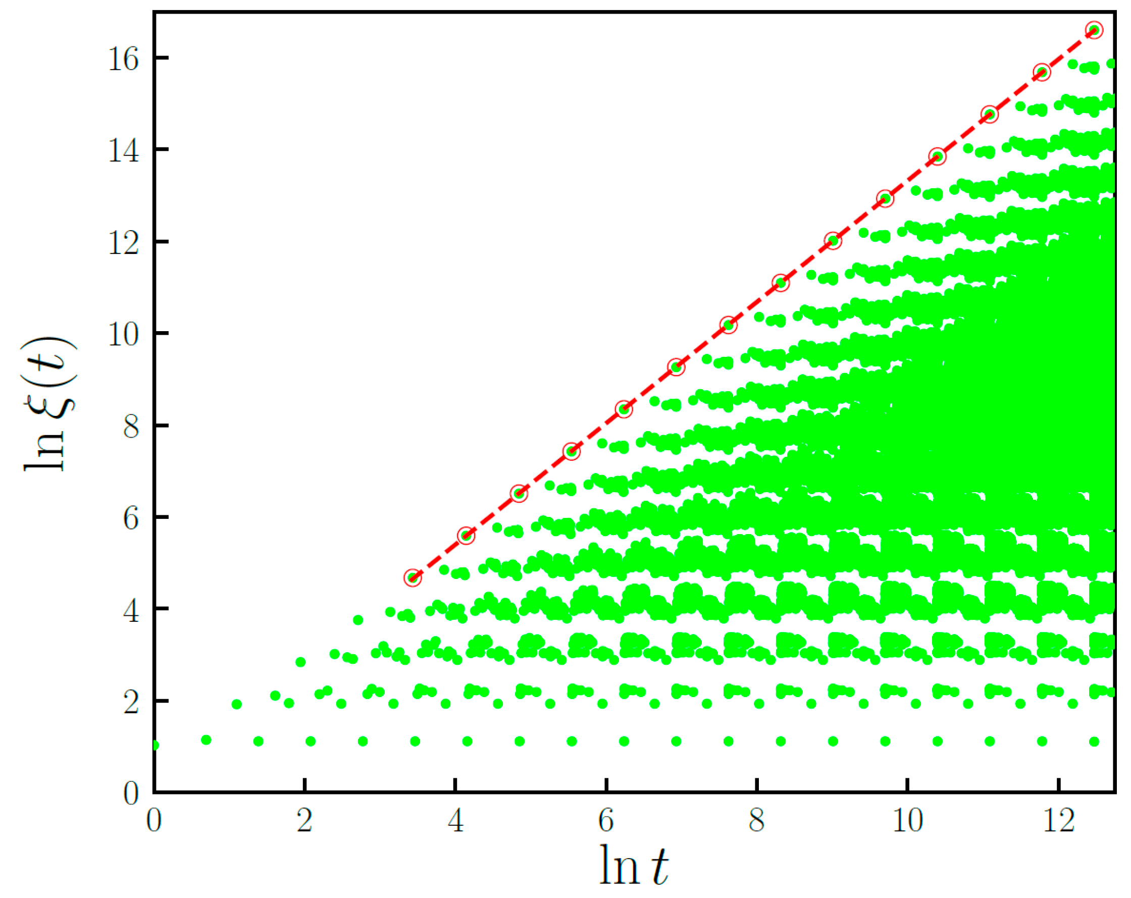
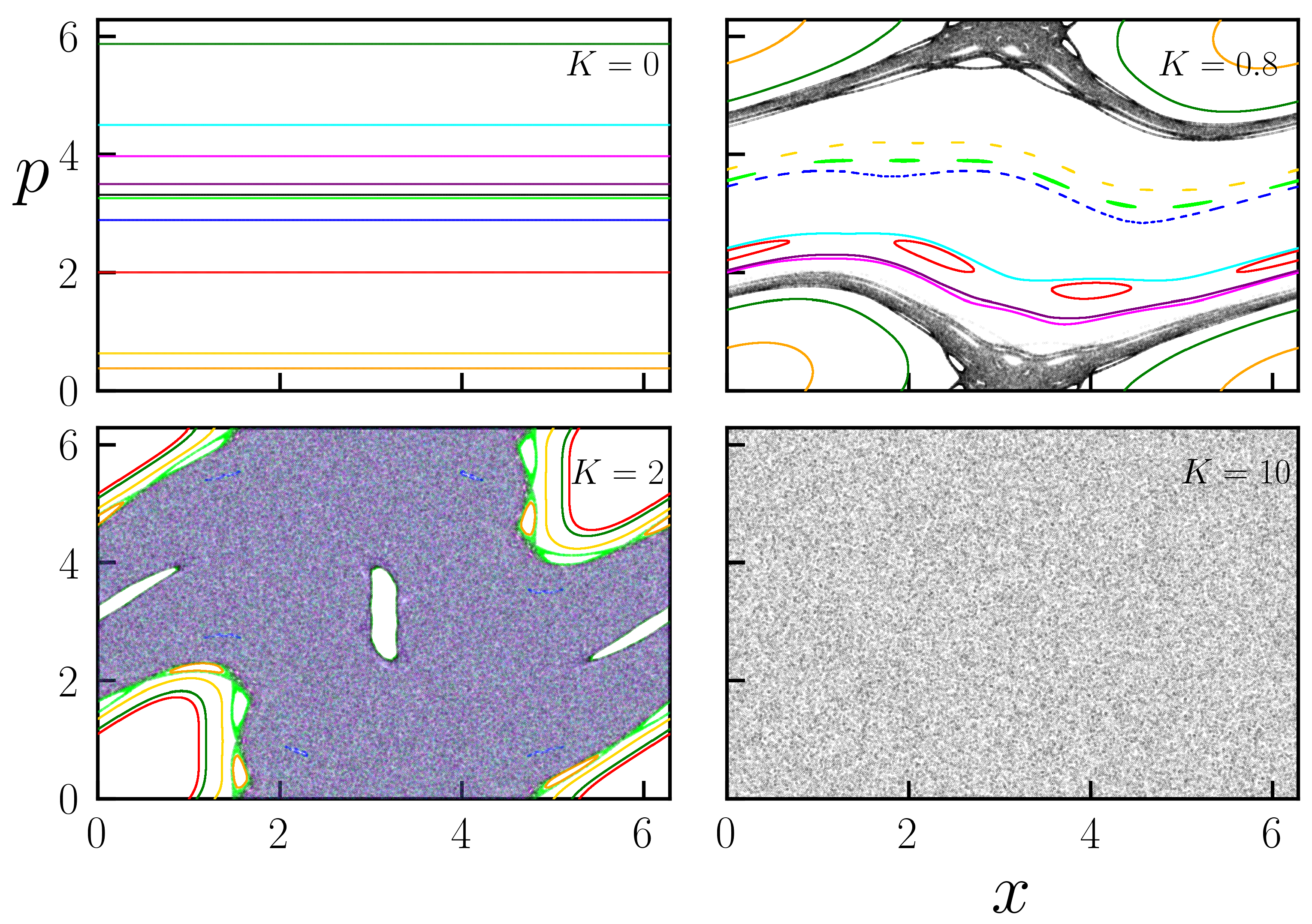
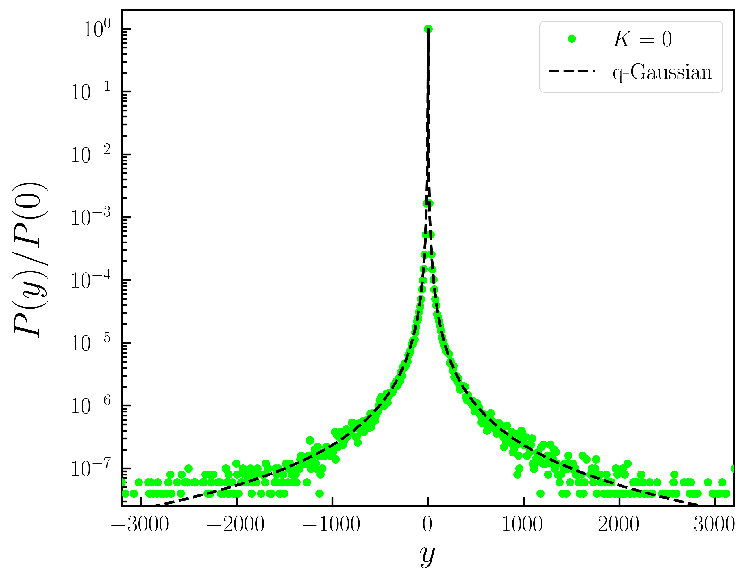
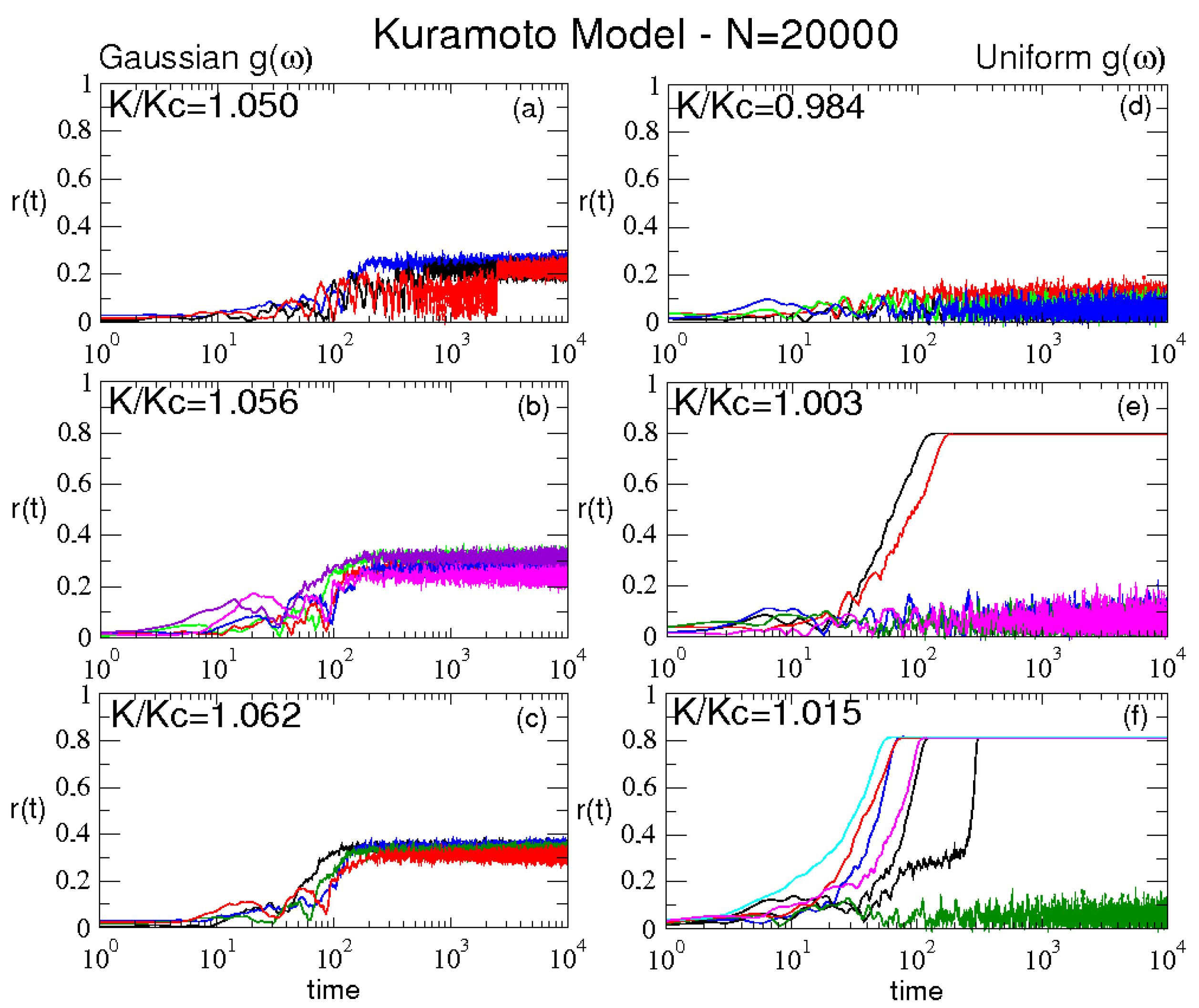
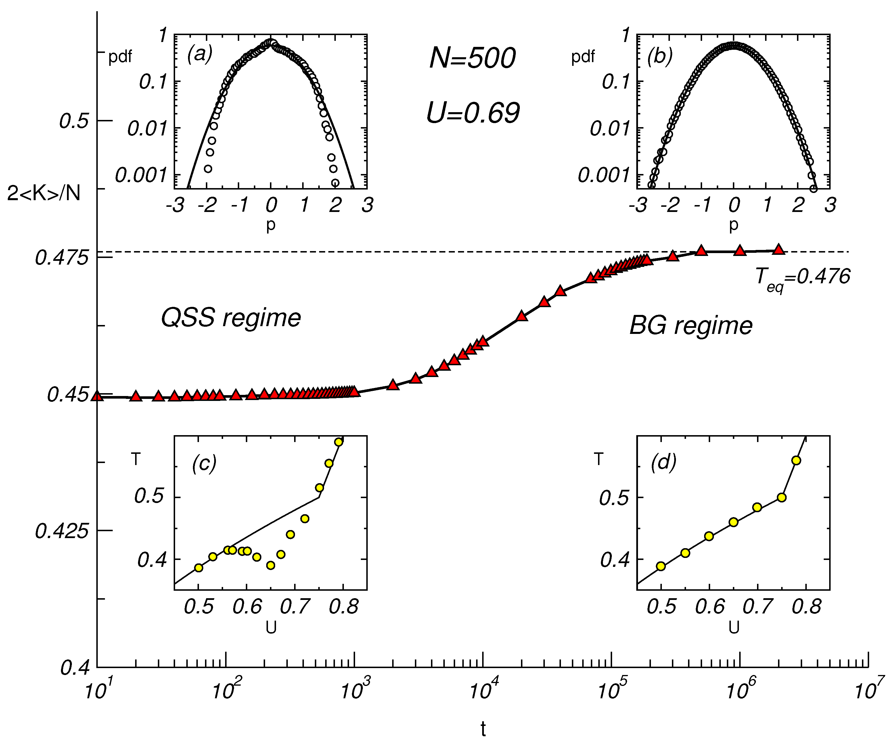
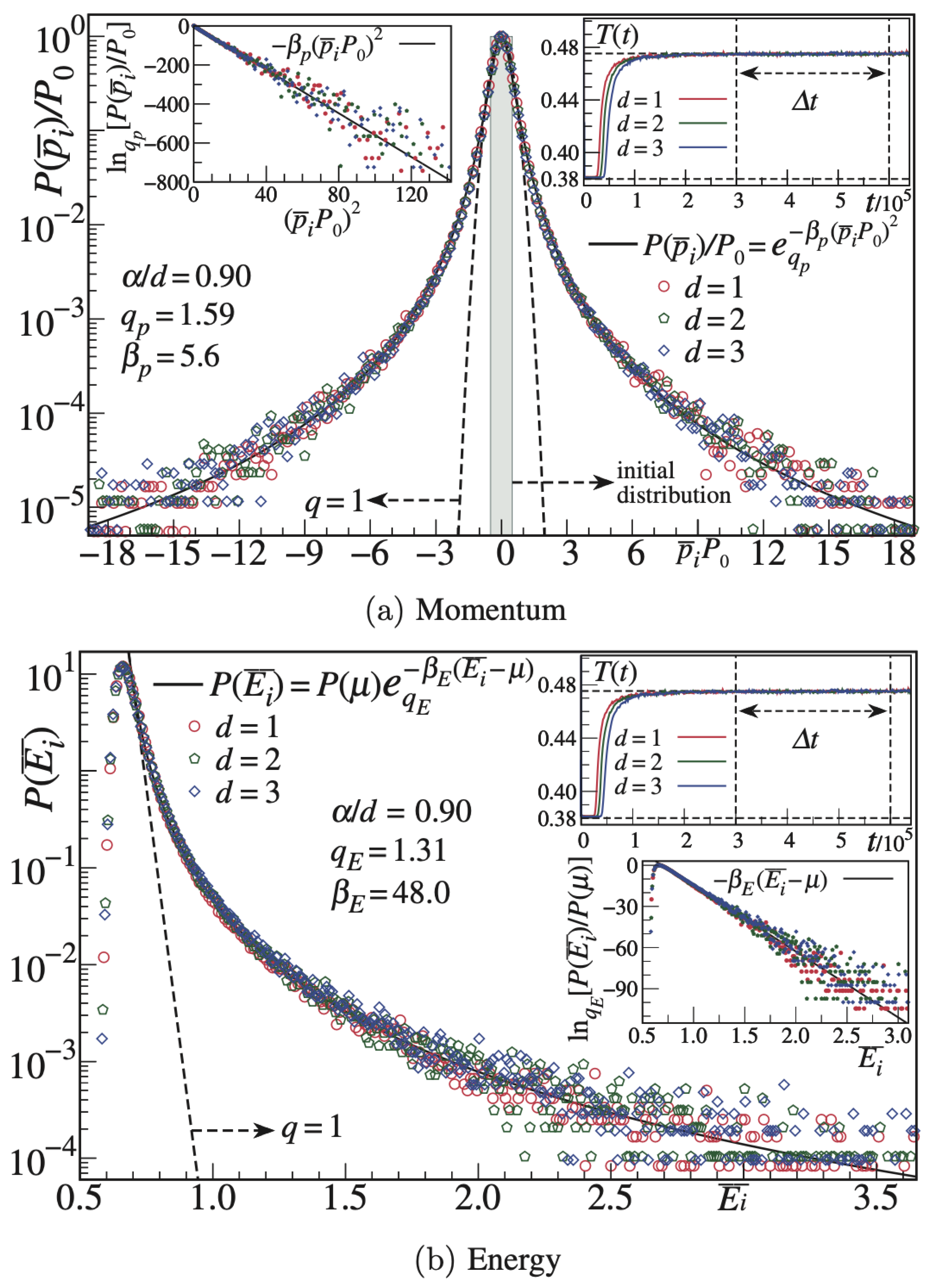
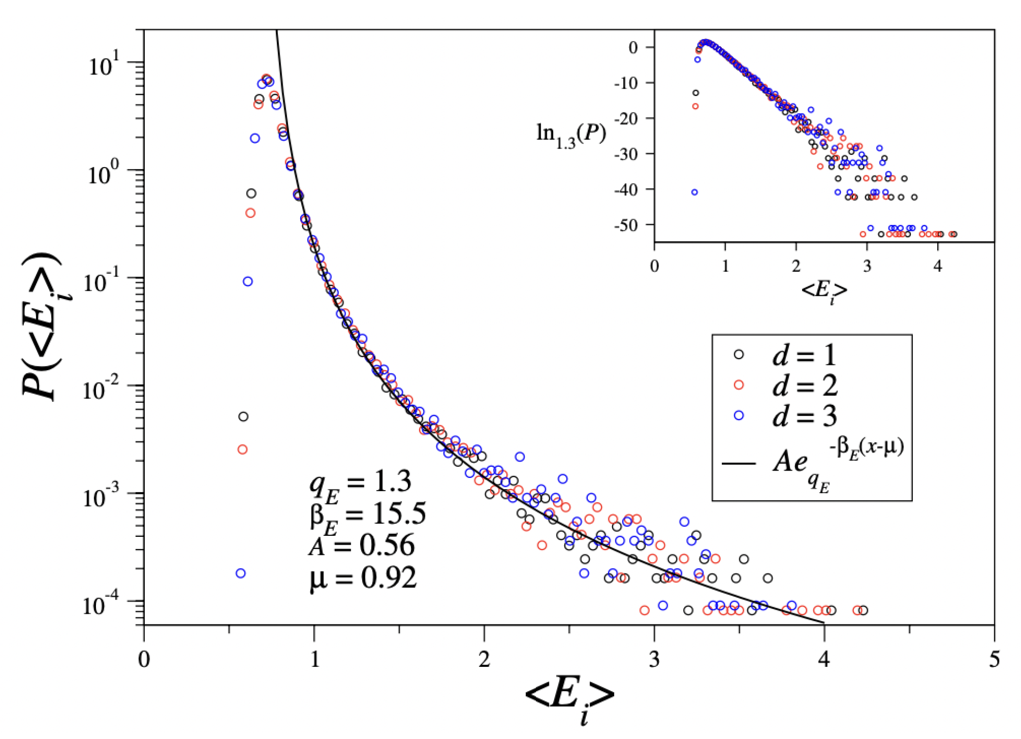
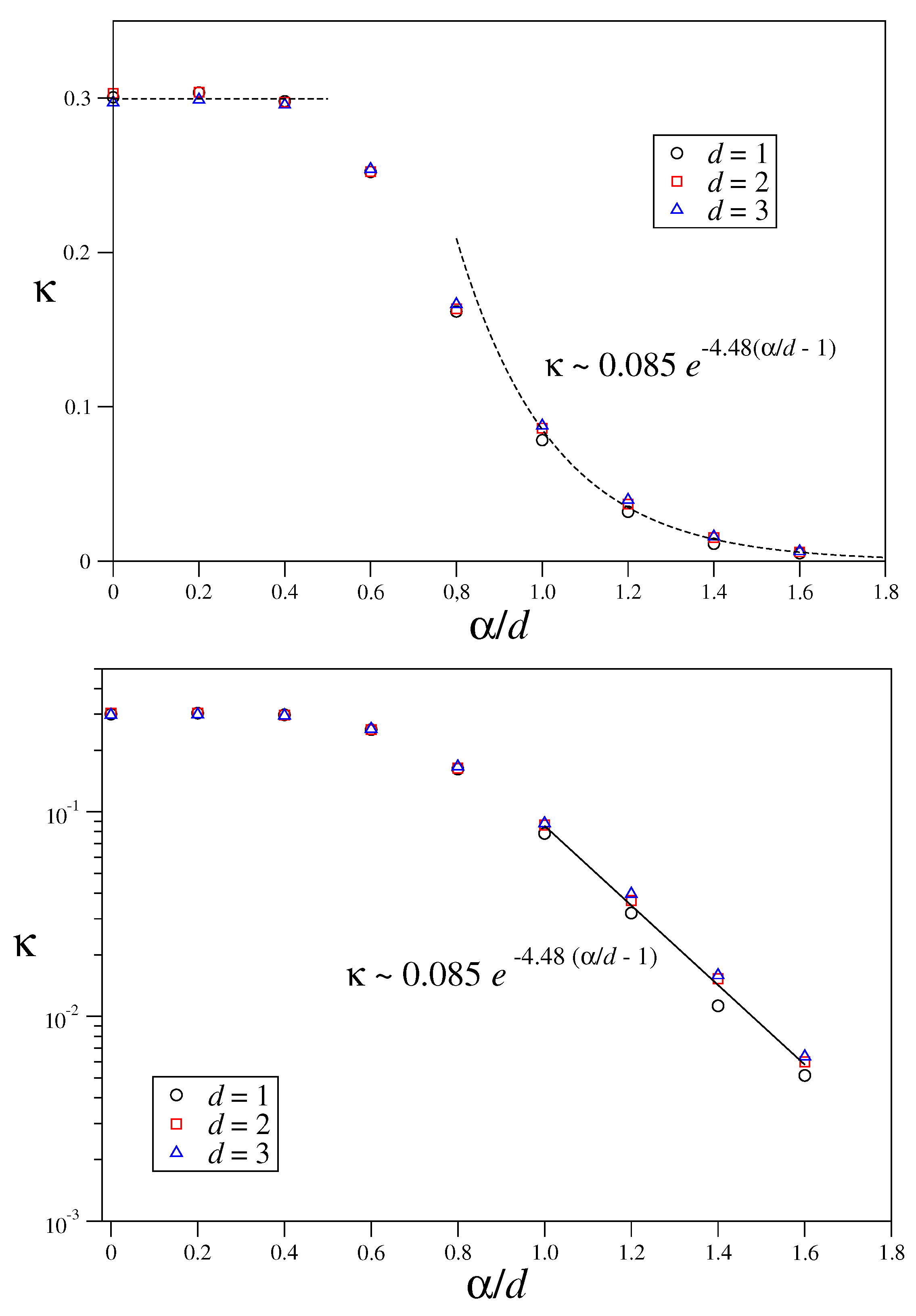
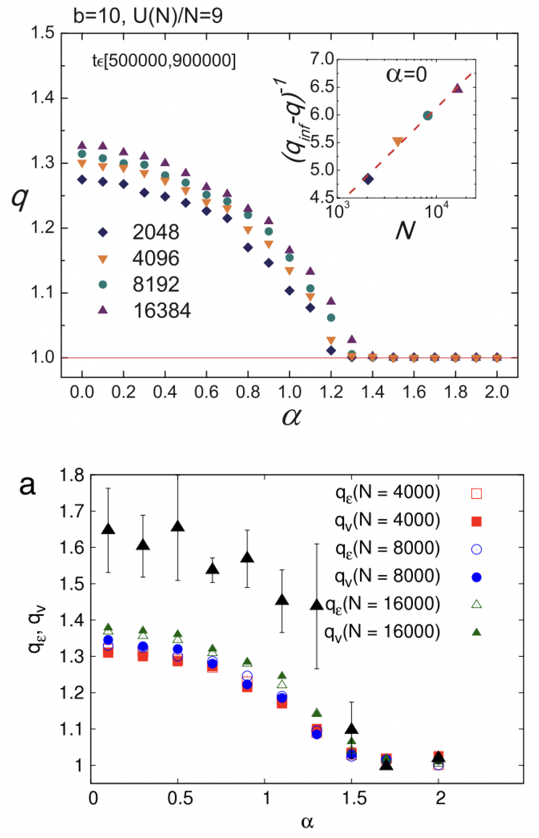
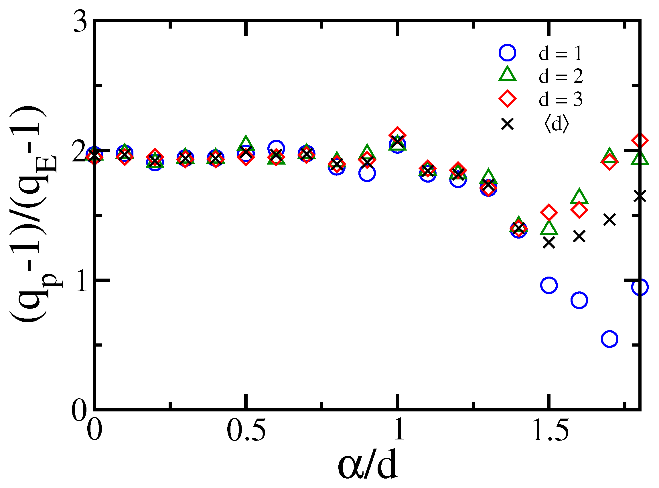
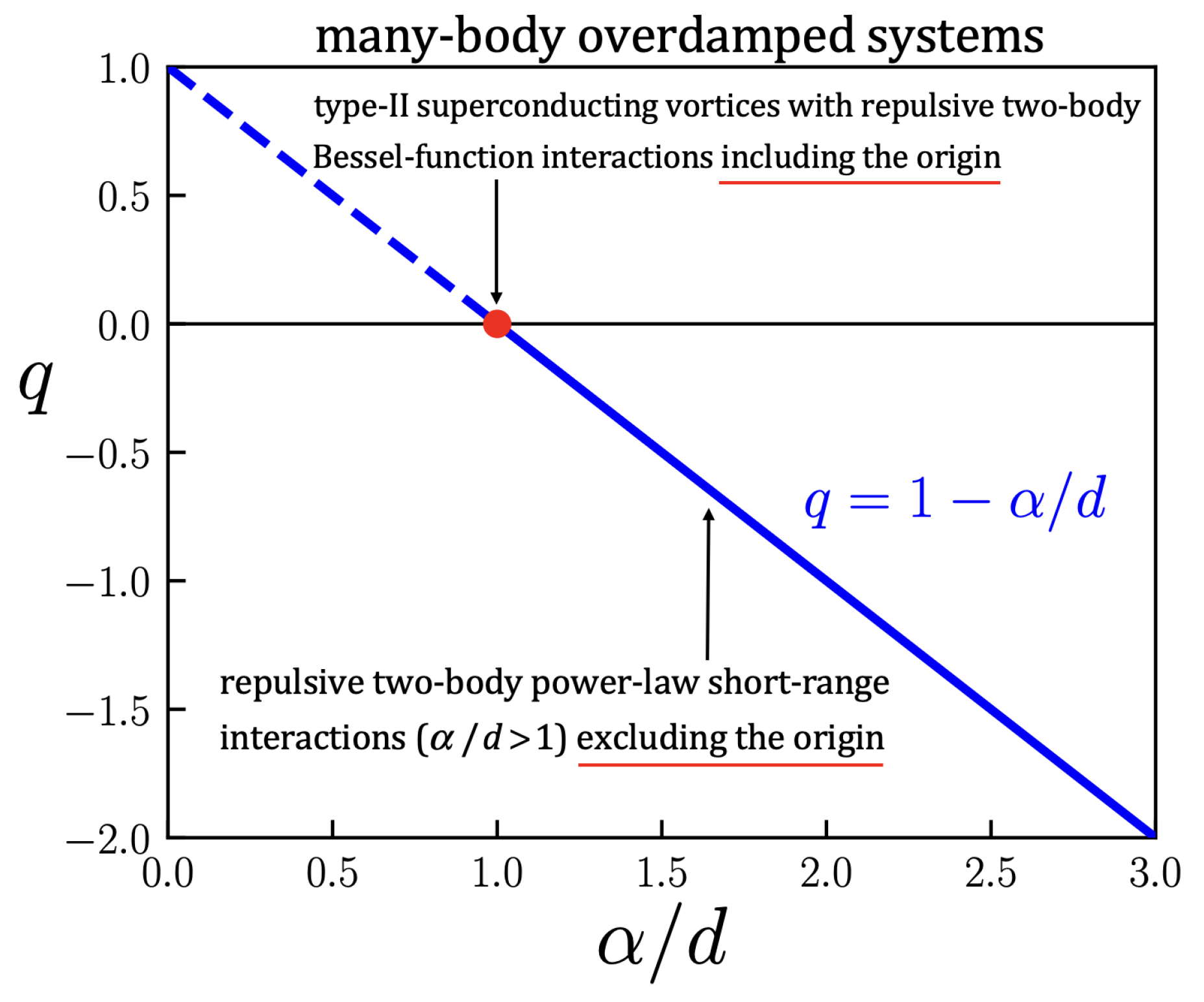
Disclaimer/Publisher’s Note: The statements, opinions and data contained in all publications are solely those of the individual author(s) and contributor(s) and not of MDPI and/or the editor(s). MDPI and/or the editor(s) disclaim responsibility for any injury to people or property resulting from any ideas, methods, instructions or products referred to in the content. |
© 2023 by the authors. Licensee MDPI, Basel, Switzerland. This article is an open access article distributed under the terms and conditions of the Creative Commons Attribution (CC BY) license (https://creativecommons.org/licenses/by/4.0/).
Share and Cite
MDPI and ACS Style
Rodríguez, A.; Pluchino, A.; Tirnakli, U.; Rapisarda, A.; Tsallis, C. Nonextensive Footprints in Dissipative and Conservative Dynamical Systems. Symmetry 2023, 15, 444. https://doi.org/10.3390/sym15020444
AMA Style
Rodríguez A, Pluchino A, Tirnakli U, Rapisarda A, Tsallis C. Nonextensive Footprints in Dissipative and Conservative Dynamical Systems. Symmetry. 2023; 15(2):444. https://doi.org/10.3390/sym15020444
Chicago/Turabian StyleRodríguez, Antonio, Alessandro Pluchino, Ugur Tirnakli, Andrea Rapisarda, and Constantino Tsallis. 2023. "Nonextensive Footprints in Dissipative and Conservative Dynamical Systems" Symmetry 15, no. 2: 444. https://doi.org/10.3390/sym15020444
Note that from the first issue of 2016, this journal uses article numbers instead of page numbers. See further details here.