
New Generalized Weibull Inverse Gompertz Distribution: Properties and Applications

Department of Statistics, Faculty of Science, King Abdulaziz University, Jeddah 21589, Saudi Arabia
Symmetry 2024, 16(2), 197; https://doi.org/10.3390/sym16020197
Submission received: 12 December 2023
/
Revised: 17 January 2024
/
Accepted: 5 February 2024
/
Published: 7 February 2024
(This article belongs to the Special Issue Selected Papers Symmetry 2023—The Fourth Edition of the International Conference on Symmetry)
Abstract
:In parametric statistical modeling, it is essential to create generalizations of current statistical distributions that are more flexible when modeling actual data sets. Therefore, this study introduces a new generalized lifetime model named the odd Weibull Inverse Gompertz distribution (OWIG). The OWIG is derived by combining the odd Weibull family of distributions with the inverse Gompertz distribution. Essential statistical properties are discussed, including reliability functions, moments, Rényi entropy, and order statistics. The proposed OWIG is particularly significant as its hazard rate functions exhibit various monotonic and nonmonotonic shapes. This enables OWIG to model different hazard behaviors more commonly observed in natural phenomena. OWIG’s parameters are estimated and its flexibility in predicting unique symmetric and asymmetric patterns is shown by analyzing real-world applications from psychology, environmental, and medical sciences. The results demonstrate that the proposed OWIG is an excellent candidate as it provides the most accurate fits to the data compared with some competing models.
1. Introduction
Many real-world problems do not fit the well-known probability models, despite the availability of well-known statistical models. Therefore, it is essential to develop probability models that more accurately capture the behavior of certain real-world phenomena.
Recently, generated families of distributions provide the potential for modeling real data with great flexibility. In addition to improving their applicability to real-life phenomena, adding new parameters to established distributions improves their ability to characterize tail shapes more accurately. Previous studies using novel approaches have generated several distributions and families of distributions. These include the beta-G family by [1], Kumaraswamy-G family by [2], Weibull-G (WG) by [3], exponentiated Weibull-G by [4], and the more general T-X family introduced by [5], among many others.
Here, we concentrate on the WG family in [3], in which the cumulative distribution function (cdf) and the probability density function (pdf) are, respectively, obtained using the T-X method as follows:
where G(x) and g(x) are the cdf and pdf of any continuous distribution, respectively. The Weibull generator’s extra parameters are sought as a way to generate more flexible distributions. The WG family provides various hazard rate function (hrf) shape characteristics and a variety of lifetime data types can be evaluated using it. Several studies have used the Weibull generator to introduce new distributions such as the Weibull Rayleigh [6], Weibull Fréchet [7], and odd Weibull inverse Topp–Leone [8].
The Gompertz distribution (GD), named after Benjamin Gompertz, has an exponentially growing failure rate [9,10]. Demographers and actuaries frequently use GD to represent the distribution of adult lifespans [11,12]. Also, GD is used to analyze survival data in several scientific disciplines, including biology, computer programming, marketing, network theory, engineering, behavioral sciences, and gerontology [13,14,15,16,17,18,19].
Unfortunately, GD’s increasing failure rate decreased its flexibility and ability to describe numerous occurrences in various domains. To compensate for these limits, a modified variant of GD with an upside-down bathtub shape hrf, called the inverse Gompertz distribution (IG), is introduced by [20]. The cdf and pdf of the IG distribution are expressed, respectively, as
In recent years, some generalizations of the IG distribution have been introduced to increase its flexibility. For example, the Kumaraswamy inverse Gompertz [21], exponentiated generalized inverted Gompertz [22], extended inverse Gompertz [23], and inverse power Gompertz [24].
The primary goal of this research is to investigate a new lifetime distribution called the Odd Weibull Inverse Gompertz distribution (OWIG), which is based on the Weibull generator and IG distribution. Including additional parameters will help with the IG distribution’s inability to fit real-world data that showed non-monotone failure rates. Therefore, the motivation for introducing OWIG distribution arises from the need to
- Increase IG’s flexibility by introducing new generalizations.
- Add greater versatility for modeling real-world data in numerous fields.
- Modeling different forms of hrf, which will help provide a “more effective fit” in many practical scenarios.
This article is outlined as follows: Section 2 and Section 3 introduce OWIG distribution and drive some of its theoretical features, with a focus on those that could be broadly significant in probability and statistics. To estimate OWIG’s parameters, the maximum likelihood (ML) technique is used in Section 4, and the performance of the estimators is examined with simulation studies in Section 5. The effectiveness of the OWIG distribution in comparison with certain competing distributions is demonstrated in Section 6 using real data sets from various fields. Finally, some concluding remarks are presented in Section 7.
2. Odd Weibull Inverse Gompertz Distribution
The cdf of OWIG can be obtained by replacing the in (1) by (4) as follows:
The corresponding pdf of OWIG is obtained by replacing and in (2) by (3) and (4), as
The Survival, , and hrf of OWIG are expressed as
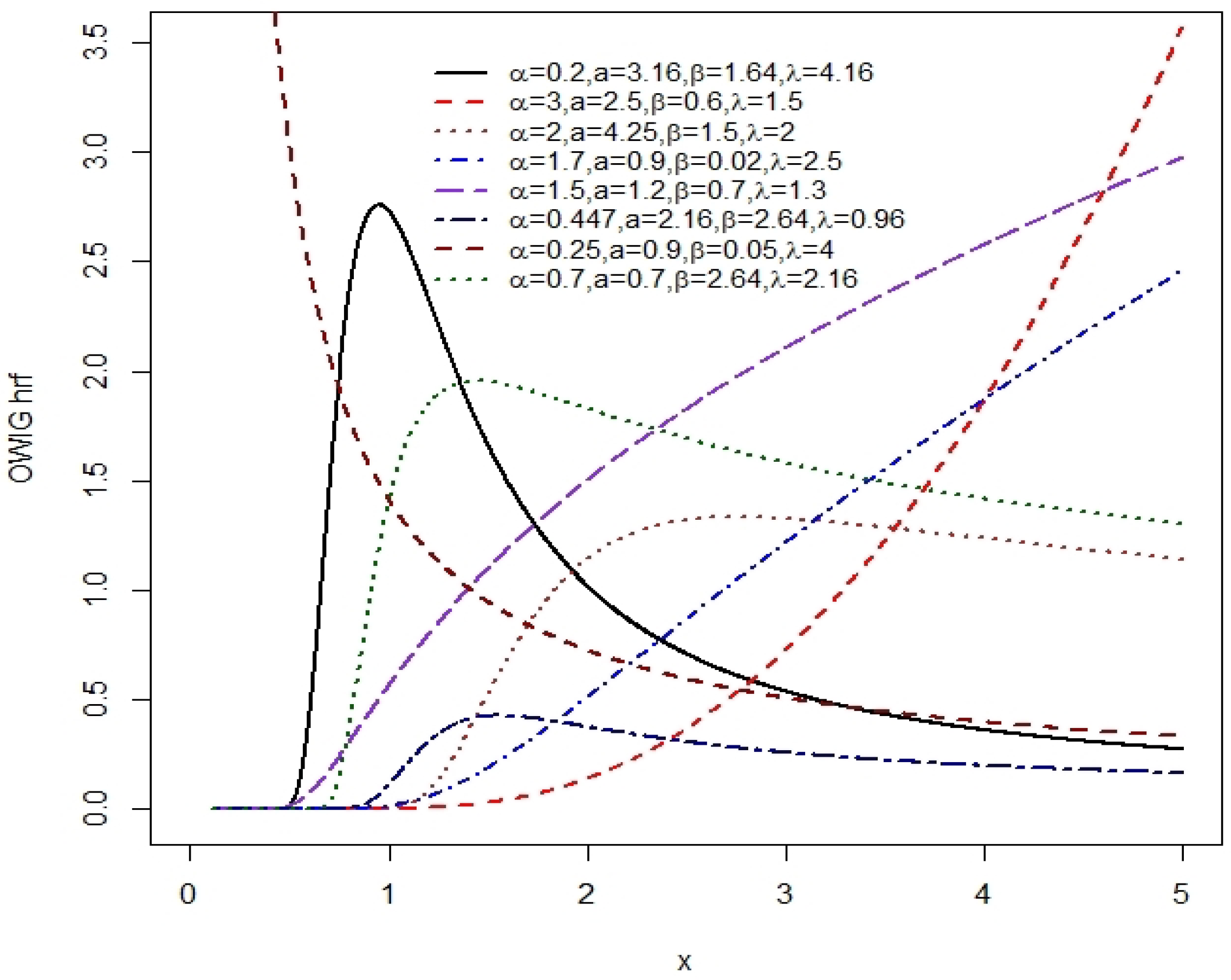
Figure 1 and Figure 2 show the various forms of OWIG’s density and hrf at some values of the parameters. The pdf of OWIG in Figure 1 shows left-skewed, symmetrical, asymmetrical, and J-shaped densities. In addition, OWIG’s hrf is attractive, as seen in Figure 2 as it exhibits a wide range of asymmetrical forms, including increasing, bath-tab, upside down bath-tab, decreasing, and reversed J-shapes. As a result, OWIG may be deemed to be a suitable model for fitting a wide range of lifetime data in practical applications.
3. Statistical Properties of the OWIG
This section investigates some essential statistical properties of OWIG.
3.1. Useful Expansions for OWIG’s Density
This subsection provides expansions for OWIG’s density provided in Equation (6) by first considering the following expansion, defined as
Then, the pdf of OWIG will become
The negative binomial series formula is defined by
Employing (11), OWIG’s pdf in Equation (10) is rewritten as
Moreover, applying (9), then
Additionally, by employing both (9) and (11), the pdf of OWIG is reduced to
where
3.2. Quantile Function
The quantile function, , of OWIG is expressed as
Therefore, OWIG’s median can be obtained as
Hence, the 25th and 75th percentiles of OWIG are obtained by replacing p by , respectively, in (14).
3.3. The Galton Skewness and Moors Kurtosis
3.4. Moments
3.5. Moment Generating Function
The OWIG’s moment-generating function (MGF) is obtained as
where is given by (13).
3.6. Characteristic Function
OWIG’s characteristic function is obtained as follows:
where is provided by (13).
3.7. Rényi Entropy
Entropies are measures of the variability or uncertainty of a R.V.X. The Rényi entropy, denoted by , is formulated as
Therefore, using the pdf of OWIG in (6), is expressed as
Applying similar concepts in Section 3.1 and using both (11) and (9), then
where
By setting , the Rényi entropy of the OWIG, is provided by
3.8. Order Statistics
4. ML Estimation
Let be am R.S. from OWIG. The log-likelihood (ℓ) for , can be written as follows
5. Simulation Studies
A Monte Carlo simulation is conducted to illustrate the performance of MLE of the OWIG parameters based on their mean square error (MSE) and root mean square error (RMSE) using the following expression:
where,
The simulation results are conducted via R program by generating 1000 samples from OWIG using the quantile function provided in Equation (14). Also, by using different sample sizes when , and 500 and several values of true parameters are obtained, as follows:
Case I:
Case II:
Case III:
Case IV:
6. Applications
The efficacy of OWIG is investigated by examining three data sets from different disciplines. The data are listed as follows:
Data 1: Pre-schoolers data
The following are the General Rating of Affective Symptoms for Preschoolers (GRASP) scores, which indicate how children’s emotional and behavioral issues are measured (frequency in parentheses) [27]:
| 19 (16) | 20 (15) | 21 (14) | 22 (9) | 23 (12) | 24 (10) | 25 (6) | 26 (9) | 27 (8) | 28 (5) | 29 (6) |
| 30 (4) | 31 (3) | 32 (4) | 33 | 34 | 35 (4) | 36 (2) | 37 (2) | 39 | 42 | 44 |
Data 2: Precipitation data
The following is the precipitation data, which represents the annual maximum precipitation (inches) in Fort Collins, Colorado, for one rain gauge (1900–1999) [28]:
| 239 | 232 | 434 | 85 | 302 | 174 | 170 | 121 | 193 | 168 | 148 | 116 | 132 |
| 132 | 144 | 183 | 223 | 96 | 298 | 97 | 116 | 146 | 84 | 230 | 138 | 170 |
| 117 | 115 | 132 | 125 | 156 | 124 | 189 | 193 | 71 | 176 | 105 | 93 | 354 |
| 60 | 151 | 160 | 219 | 142 | 117 | 87 | 223 | 215 | 108 | 354 | 213 | 306 |
| 169 | 184 | 71 | 98 | 96 | 218 | 176 | 121 | 161 | 321 | 102 | 269 | 98 |
| 271 | 95 | 212 | 151 | 136 | 240 | 162 | 71 | 110 | 285 | 215 | 103 | 443 |
| 185 | 199 | 115 | 134 | 297 | 187 | 203 | 146 | 94 | 129 | 162 | 112 | 348 |
| 95 | 249 | 103 | 181 | 152 | 135 | 463 | 183 | 241 |
Data 3: Survival times of cancer patients
The survival rates for 44 people with head and neck cancer are listed below. Chemotherapy and radiation (RT+CT) are used to treat patients [28]:
| 12.20 | 23.56 | 23.74 | 25.87 | 31.98 | 37 | 41.35 | 47.38 | 55.46 | 58.36 | 63.47 | 68.46 |
| 78.26 | 74.47 | 81.43 | 84 | 92 | 94 | 110 | 112 | 119 | 127 | 130 | 133 |
| 140 | 146 | 155 | 159 | 173 | 179 | 194 | 195 | 209 | 249 | 281 | 319 |
| 339 | 432 | 469 | 519 | 633 | 725 | 817 | 1776 |
The appropriateness of the three data sets for OWIG is evaluated by comparing its fit to the following distributions:
- The Weibull Inverse Gompertz (WIG) using the Weibull-G family in [5], where the G is represented by the IG distribution
- The generalized inverse Gompertz (GIG) by [23]
- The inverse power Gompertz (PIG) by [24]
The performance of OWIG is assessed using the goodness of fit criteria (GoF), which include the , Akaike information criterion (AIC), corrected AIC (CAIC), Bayesian information criterion (BIC), Kramér-von Mises (W*), Anderson–Darling (AD*), and Kolmog- orov–Smirnov (KS) test statistics with its corresponding p-value. In general, the model with the lowest AIC, CAIC, BIC, and KS values with the highest p-value will provide a better fit for the data.
Table 3, Table 4 and Table 5 present the MLEs, as well as the GoF criteria of OWIG and the competing distributions for all datasets. Furthermore, the estimated pdf and cdf of OWIG and rival distributions are shown in Figure 3, Figure 4 and Figure 5.
Concerning Tables Table 3, Table 4 and Table 5, OWIG has the largest p-value and the lowest values of GOF criteria. This suggests that OWIG provides better fits for all three applications when compared with the rival distributions. Figure 3, Figure 4 and Figure 5 also clearly show that OWIG matches the histogram more closely than the other competitive distributions.
7. Conclusions
This work introduced the OWIG distribution derived by considering the Weibull generator with the IG distribution. This is regarded as a new generalization of the IG distribution. The proposed OWIG is more versatile as its density and hrf present attractive shapes. The OWIG’s hrf includes increasing, bath-tab, upside down bath-tab, decreasing, reversed J-shape, and unimodal shapes, which are suitable to fit an extensive variety of real data behaviors. Some essential statistical properties of OWIG are obtained. The well-known ML approach is utilized to estimate the parameters of OWIG, and the performance of the ML estimators is examined using Monte Carlo simulation studies. The simulation results confirmed that the ML estimation approach functioned effectively for estimating the OWIG parameters. Three real data sets from psychology, environmental, and medical sciences are analyzed to determine the OWIG’s modeling capability and efficiency, demonstrating that it can fit data more accurately than WIG, GIG, PIG, and IG. OWIG has the highest p-value of KS statistics and the lowest GoF criterion for the three data. Compared with many lifetime models, the proposed OWIG will be capable of providing a superior fit for many lifetime and reliability applications.
Funding
This research received no external funding.
Data Availability Statement
Publicly available datasets were analyzed in this study. The data can be found in the cited references.
Conflicts of Interest
The author declares no conflicts of interest.
References
- Eugene, N.; Lee, C.; Famoye, F. Beta-normal distribution and its applications. Commun. Stat. Theory Methods 2002, 31, 497–512. [Google Scholar] [CrossRef]
- Cordeiro, G.M.; de Castro, M. A new family of generalized distributions. J. Stat. Comput. Simul. 2011, 81, 883–898. [Google Scholar] [CrossRef]
- Bourguignon, M.; Silva, R.B.; Cordeiro, G.M. The Weibull-G family of probability distributions. J. Data Sci. 2014, 12, 53–68. [Google Scholar] [CrossRef]
- Cordeiro, G.M.; Afify, A.Z.; Yousof, H.M.; Pescim, R.R.; Aryal, G.R. The exponentiated Weibull-H family of distributions: Theory and Applications. Mediterr. J. Math. 2017, 14, 155. [Google Scholar] [CrossRef]
- Alzaatreh, A.; Lee, C.; Famoye, F. A new method for generating families of continuous distributions. Metron 2013, 71, 63–79. [Google Scholar] [CrossRef]
- Merovci, F.; Elbatal, I. Weibull Rayleigh distribution: Theory and applications. Appl. Math. Inf. Sci 2015, 9, 1–11. [Google Scholar]
- Afify, A.Z.; Yousof, H.M.; Cordeiro, G.M.; M Ortega, E.M.; Nofal, Z.M. The Weibull Fréchet distribution and its applications. J. Appl. Stat. 2016, 43, 2608–2626. [Google Scholar] [CrossRef]
- Almetwally, E.M. The odd Weibull inverse topp–leone distribution with applications to COVID-19 data. Ann. Data Sci. 2022, 9, 121–140. [Google Scholar] [CrossRef]
- Gompertz, B. XXIV. On the nature of the function expressive of the law of human mortality, and on a new mode of determining the value of life contingencies. In a letter to Francis Baily, Esq. FRS &c. In Philosophical Transactions of the Royal Society of London; The Royal Society: London, UK, 1825; pp. 513–583. [Google Scholar]
- Pollard, J.H.; Valkovics, E.J. The Gompertz distribution and its applications. Genus 1992, 48, 15–28. [Google Scholar] [PubMed]
- Leridon, H. Demography: Measuring and Modeling Population Processes; Population Council: Washington, DC, USA, 2001. [Google Scholar]
- Willemse, W.J.; Koppelaar, H. Knowledge elicitation of Gompertz’law of mortality. Scand. Actuar. J. 2000, 2000, 168–179. [Google Scholar] [CrossRef]
- El-Bassiouny, A.; El-Damcese, M.; Mustafa, A.; Eliwa, M. Exponentiated generalized Weibull-Gompertz distribution with application in survival analysis. J. Stat. Appl. Probab 2017, 6, 7–16. [Google Scholar] [CrossRef]
- El-Gohary, A.; Alshamrani, A.; Al-Otaibi, A.N. The generalized Gompertz distribution. Appl. Math. Model. 2013, 37, 13–24. [Google Scholar] [CrossRef]
- Franses, P.H. Fitting a Gompertz curve. J. Oper. Res. Soc. 1994, 45, 109–113. [Google Scholar] [CrossRef]
- Khan, M.S.; Robert, K.; Irene, L. Transmuted Gompertz distribution: Properties and estimation. Pak. J. Stat. 2016, 32, 161–182. [Google Scholar]
- Roozegar, R.; Tahmasebi, S.; Jafari, A.A. The McDonald Gompertz distribution: Properties and applications. Commun. Stat.-Simul. Comput. 2017, 46, 3341–3355. [Google Scholar] [CrossRef]
- Dey, S.; Kayal, T.; Tripathi, Y.M. Evaluation and comparison of estimators in the Gompertz distribution. Ann. Data Sci. 2018, 5, 235–258. [Google Scholar] [CrossRef]
- Asadi, S.; Panahi, H.; Swarup, C.; Lone, S.A. Inference on adaptive progressive hybrid censored accelerated life test for Gompertz distribution and its evaluation for virus-containing micro droplets data. Alex. Eng. J. 2022, 61, 10071–10084. [Google Scholar] [CrossRef]
- Eliwa, M.; El-Morshedy, M.; Ibrahim, M. Inverse Gompertz distribution: Properties and different estimation methods with application to complete and censored data. Ann. Data Sci. 2019, 6, 321–339. [Google Scholar] [CrossRef]
- El-Morshedy, M.; El-Faheem, A.A.; El-Dawoody, M. Kumaraswamy inverse Gompertz distribution: Properties and engineering applications to complete, type-II right censored and upper record data. PLoS ONE 2020, 15, e0241970. [Google Scholar] [CrossRef] [PubMed]
- El-Morshedy, M.; El-Faheem, A.A.; Al-Bossly, A.; El-Dawoody, M. Exponentiated generalized inverted gompertz distribution: Properties and estimation methods with applications to symmetric and asymmetric data. Symmetry 2021, 13, 1868. [Google Scholar] [CrossRef]
- Elshahhat, A.; Aljohani, H.M.; Afify, A.Z. Bayesian and classical inference under type-II censored samples of the extended inverse Gompertz distribution with engineering applications. Entropy 2021, 23, 1578. [Google Scholar] [CrossRef] [PubMed]
- Abdelhady, D.H.; Amer, Y.M. On the inverse power Gompertz distribution. Ann. Data Sci. 2021, 8, 451–473. [Google Scholar] [CrossRef]
- Galton, F. Inquiries into Human Faculty and Its Development; Macmillan: London, UK, 1883. [Google Scholar]
- Moors, J. A quantile alternative for kurtosis. J. R. Stat. Soc. Ser. D (Stat.) 1988, 37, 25–32. [Google Scholar] [CrossRef]
- Almetwally, E.M.; Alharbi, R.; Alnagar, D.; Hafez, E.H. A new inverted topp-leone distribution: Applications to the COVID-19 mortality rate in two different countries. Axioms 2021, 10, 25. [Google Scholar] [CrossRef]
- Katz, R.W.; Parlange, M.B.; Naveau, P. Statistics of extremes in hydrology. Adv. Water Resour. 2002, 25, 1287–1304. [Google Scholar] [CrossRef]
Figure 1.
The plots for the OWIG pdf for some certain values.

Figure 2.
OWIG’s hrf plots at some selected values.

Figure 3.
Estimated cdfs and pdfs for GRASP data.

Figure 4.
Estimated cdfs and pdfs for precipitation data.

Figure 5.
Estimated cdfs and pdfs for cancer data.


Table 1.
Simulation study: Parameter estimates, MSE, and RMSE for case I and case II.
| Sample Size | Parameter | Case I | Case II | ||||
|---|---|---|---|---|---|---|---|
| Estimate | MSE | RMSE | Estimate | MSE | RMSE | ||
| n = 50 | 1.9142 | 0.3997 | 0.6322 | 0.8690 | 0.0586 | 0.2421 | |
| a | 0.4209 | 0.6975 | 0.8352 | 1.0842 | 3.5263 | 1.8778 | |
| 0.6130 | 0.3843 | 0.6199 | 0.9822 | 1.0892 | 1.0437 | ||
| 0.1735 | 0.0621 | 0.2493 | 1.0883 | 2.8870 | 1.6991 | ||
| n = 100 | 0.6880 | 0.0049 | 0.0702 | 0.8745 | 0.0298 | 0.1728 | |
| a | 0.4195 | 0.3496 | 0.5913 | 1.0149 | 2.2070 | 1.4856 | |
| 0.4756 | 0.1924 | 0.4387 | 0.8286 | 0.6433 | 0.8021 | ||
| 0.1698 | 0.0360 | 0.1896 | 1.0241 | 1.7828 | 1.3352 | ||
| n = 200 | 0.6923 | 0.0024 | 0.0494 | 0.8889 | 0.0156 | 0.1248 | |
| a | 0.4258 | 0.2052 | 0.4530 | 0.9865 | 0.9415 | 0.9703 | |
| 0.4011 | 0.1276 | 0.3572 | 0.6753 | 0.4045 | 0.6360 | ||
| 0.1714 | 0.0231 | 0.1521 | 1.0205 | 1.0337 | 1.0167 | ||
| n = 500 | 0.6976 | 0.0009 | 0.0307 | 0.8956 | 0.0076 | 0.0872 | |
| a | 0.4216 | 0.1029 | 0.3208 | 1.0151 | 0.4463 | 0.6680 | |
| 0.3288 | 0.0720 | 0.2684 | 0.5313 | 0.2020 | 0.4494 | ||
| 0.1704 | 0.0118 | 0.1088 | 1.0395 | 0.5193 | 0.7206 | ||
Table 2.
Simulation study: Parameter estimates, MSE, and RMSE for case III and case IV.
| Sample Size | Parameter | Case III | Case IV | ||||
|---|---|---|---|---|---|---|---|
| Estimate | MSE | RMSE | Estimate | MSE | RMSE | ||
| n = 50 | 1.9452 | 0.4048 | 0.6363 | 1.8989 | 0.3381 | 0.5814 | |
| a | 1.5665 | 5.2237 | 2.2855 | 0.4679 | 0.2520 | 0.5020 | |
| 5.8516 | 27.9653 | 5.2882 | 1.9143 | 3.2040 | 1.7900 | ||
| 0.3557 | 3.1456 | 1.7736 | 0.2428 | 1.0497 | 1.0245 | ||
| n = 100 | 1.9801 | 0.1765 | 0.4202 | 1.9668 | 0.1699 | 0.4122 | |
| a | 1.4780 | 2.7060 | 1.6450 | 0.5088 | 0.2192 | 0.4682 | |
| 4.9706 | 11.2436 | 3.3532 | 1.5100 | 1.1033 | 1.0504 | ||
| 0.2225 | 1.2119 | 1.1009 | 0.2230 | 0.5908 | 0.7686 | ||
| n = 200 | 1.9557 | 0.0829 | 0.2879 | 1.9545 | 0.0855 | 0.2925 | |
| a | 1.5413 | 1.1824 | 1.0874 | 0.5213 | 0.1734 | 0.4164 | |
| 4.6192 | 5.2342 | 2.2878 | 1.4016 | 0.5594 | 0.7479 | ||
| 0.1880 | 0.2274 | 0.4768 | 0.2164 | 0.4497 | 0.6706 | ||
| n = 500 | 1.9712 | 0.0323 | 0.1796 | 1.9688 | 0.0326 | 0.1805 | |
| a | 1.5281 | 0.7382 | 0.8592 | 0.5113 | 0.0892 | 0.2987 | |
| 4.3456 | 2.2659 | 1.5053 | 1.3180 | 0.2617 | 0.5115 | ||
| 0.1547 | 0.0946 | 0.3076 | 0.1546 | 0.0738 | 0.2717 | ||
Table 3.
MLEs and GoF measures for GRASP data.
| Distributions | OWIG | WIG | GIG | PIG | IG |
|---|---|---|---|---|---|
| Estimates | 4.5623 | 0.1231 | |||
| 0.4747 | 0.9684 | 1.5841 | 5.2337 | ||
| 0.0062 | 0.9731 | 0.0532 | 3.9800 | 0.0101 | |
| 10.9913 | 3.3355 | 7.2699 | 2.8420 | 9.4218 | |
| −15.4156 | −22.5233 | −21.6541 | −18.5220 | −21.8509 | |
| AIC | 38.8313 | 53.0465 | 49.3083 | 43.0441 | 47.7019 |
| CAIC | 44.6270 | 58.8422 | 53.6551 | 47.3908 | 50.5998 |
| BIC | 50.4227 | 64.6379 | 58.0019 | 51.7376 | 53.4976 |
| W* | 0.1231 | 0.2307 | 0.2092 | 0.2141 | 0.2177 |
| AD* | 1.0045 | 1.9120 | 1.5296 | 1.5319 | 1.6097 |
| KS | 0.0886 | 0.0891 | 0.0991 | 0.0945 | 0.0973 |
| p-value | 0.2428 | 0.2384 | 0.1385 | 0.1821 | 0.1581 |
Table 4.
MLEs and GoF measures for precipitation data.
| Distributions | OWIG | WIG | GIG | PIG | IG |
|---|---|---|---|---|---|
| Estimates | 0.9241 | 1.9389 | |||
| 1.0991 | 4.3919 | 0.8167 | 0.2891 | ||
| 79.9890 | 26.8193 | 54.4072 | 0.0071 | 40.7834 | |
| 141.2530 | 31.4120 | 16.0385 | 34.3842 | 238.2838 | |
| −564.6826 | −564.8341 | −641.5151 | −572.47 | −579.5334 | |
| AIC | 1137.365 | 1139.994 | 1289.030 | 1150.940 | 1163.067 |
| CAIC | 1142.575 | 1147.745 | 1292.938 | 1154.848 | 1165.672 |
| BIC | 1147.786 | 1152.955 | 1296.846 | 1158.755 | 1168.277 |
| W* | 0.0156 | 0.0465 | 4.3555 | 0.1391 | 0.3240 |
| AD* | 0.1524 | 0.3555 | 21.4890 | 1.1192 | 2.4481 |
| KS | 0.0407 | 0.0551 | 0.3884 | 0.0764 | 0.1215 |
| p-value | 0.9964 | 0.8714 | 1.559 | 0.6022 | 0.1041 |
Table 5.
MLEs and GoF measures for cancer data.
| Distributions | OWIG | WIG | GIG | PIG | IG |
|---|---|---|---|---|---|
| Estimates | 0.0055 | 10.5667 | |||
| 0.7541 | 14.9225 | 0.6323 | 0.6977 | ||
| 0.1596 | 0.0073 | 30.5926 | 15.8997 | 46.3294 | |
| 80.7622 | 3.4091 | 8.4041 | 8.2868 | 9.8322 | |
| −277.836 | −289.9746 | −286.0049 | −282.6561 | −283.3979 | |
| AIC | 563.6720 | 587.9493 | 578.0097 | 571.3122 | 570.7958 |
| CAIC | 567.2403 | 591.5176 | 580.686 | 573.9885 | 572.5800 |
| BIC | 570.8087 | 595.0860 | 583.3623 | 576.6648 | 574.3642 |
| W* | 0.0432 | 1.4577 | 0.6158 | 0.1885 | 0.8875 |
| AD* | 0.2655 | 7.9456 | 3.1290 | 1.2207 | 4.0556 |
| KS | 0.0908 | 0.2938 | 0.2156 | 0.1195 | 0.2415 |
| p-value | 0.8284 | 0.0007 | 0.0282 | 0.5167 | 0.0096 |
Disclaimer/Publisher’s Note: The statements, opinions and data contained in all publications are solely those of the individual author(s) and contributor(s) and not of MDPI and/or the editor(s). MDPI and/or the editor(s) disclaim responsibility for any injury to people or property resulting from any ideas, methods, instructions or products referred to in the content. |
© 2024 by the author. Licensee MDPI, Basel, Switzerland. This article is an open access article distributed under the terms and conditions of the Creative Commons Attribution (CC BY) license (https://creativecommons.org/licenses/by/4.0/).
Share and Cite
MDPI and ACS Style
Baharith, L.A. New Generalized Weibull Inverse Gompertz Distribution: Properties and Applications. Symmetry 2024, 16, 197. https://doi.org/10.3390/sym16020197
AMA Style
Baharith LA. New Generalized Weibull Inverse Gompertz Distribution: Properties and Applications. Symmetry. 2024; 16(2):197. https://doi.org/10.3390/sym16020197
Chicago/Turabian StyleBaharith, Lamya A. 2024. "New Generalized Weibull Inverse Gompertz Distribution: Properties and Applications" Symmetry 16, no. 2: 197. https://doi.org/10.3390/sym16020197
Note that from the first issue of 2016, this journal uses article numbers instead of page numbers. See further details here.