
Statistical Inference and Application of Asymmetrical Generalized Pareto Distribution Based on Peaks-Over-Threshold Model
1
School of Mathematics, Statistics and Mechanics, Beijing University of Technology, Beijing 100124, China
2
China National Environmental Monitoring Center, Beijing 100012, China
3
School of Economics, Nanjing University of Finance and Economics, Nanjing 210023, China
4
University of Chinese Academy of Sciences, Beijing 100049, China
5
Institute of Computing Technology, Chinese Academy of Sciences, Beijing 100190, China
*
Authors to whom correspondence should be addressed.
†
Current address: No.100, Pingleyuan, Chaoyang District, Beijing 100124, China.
Symmetry 2024, 16(3), 365; https://doi.org/10.3390/sym16030365
Submission received: 6 February 2024
/
Revised: 1 March 2024
/
Accepted: 8 March 2024
/
Published: 18 March 2024
(This article belongs to the Special Issue Symmetrical and Asymmetrical Distributions in Statistics and Data Science II)
Abstract
:Generalized Pareto distribution (GPD), an asymmetrical distribution, primarily models exceedances over a high threshold in many applications. Within the peaks-over-threshold (POT) framework, we consider a new GPD parameter estimation method to estimate a common tail risk measure, the value at risk (VaR). The proposed method is more suitable for the POT framework and makes full use of data information. Specifically, our estimation method builds upon the generalized probability weighted moments method and integrates it with the nonlinear weighted least squares method. We use exceedances for the GPD, minimizing the sum of squared differences between the sample and population moments of a function of GPD random variables. At the same time, the proposed estimator uses three iterations and assigns weight to further improving the estimated performance. Under Monte Carlo simulations and with a real heavy-tailed dataset, the simulation results show the advantage of the newly proposed estimator, particularly when VaRs are at high confidence levels. In addition, by simulating other heavy-tailed distributions, our method still exhibits good performance in estimating misjudgment distributions.
1. Introduction
Some scholars have found that the tails of various measured data distributions tend to be heavier than those of a normal distribution, as reported in [1,2]. Embrechts et al. [3] proposed the assumption that normal distribution will underestimate the risk associated with extreme tails. Since the 1990s, the extreme value theory (EVT) has been widely used in insurance, earthquake analysis, hydrology, transportation, climate, reliability analysis and other fields. The EVT mainly uses two approaches for modeling random variables: the block maxima model (BMM) and peaks over threshold (POT). The BMM first divides the sample interval, takes the maximum value in each sample interval, and then asymptotically fits the obtained maximum value series as the analysis object to the generalized extreme value (GEV) distributions. However, the POT fits all exceedances over a given threshold for heavy-tailed data. Pickands [4] first proposed that the excesses can be approximated via the generalized Pareto distribution (GPD) when the distribution of excesses is in the maximum domain of attraction. In the field of financial market analysis, risk measurement is an extremely important issue. As one of the most important and widely accepted risk measurement tools, Value at Risk (VaR) can reflect the risk and play an early-warning role in financial markets. The VaR from the fitted GPD is extremely sensitive to the GPD parameter estimators and a small difference in the parameter value will cause a significant impact on a bank’s financial position, highlighting the importance of accurately estimating GPD parameters.
Since Pickands first proposed the GPD, various parameter estimation methods for this distribution have been studied. For example, Hosking and Wallis [5] considered the method of moments (MOMs); Greenwood et al. [6] discussed probability weighted moments (PWMs); Smith [7] introduced maximum likelihood (ML); and Moharram et al. [8] discussed the least square (LS) of the GPD. Hosking [9] developed an L-moment method based on the PWM linear combination; Ashkar and Ouarda [10] proposed the generalized method of moments (GMOM) based on the MOM method. Castillo and Hadi [11] used the elemental percentile method (EPM). Based on the EPM, From and Ratnasingam [12] proposed various efficient closed-form estimators for the GPD. Product of spacing (POS) and logarithmic Cramér–von Mises (LCVM) methods were proposed at the same time. Rasmussen [13] proposed generalized probability weighted moments (GPWMs) based on the PWM method, both of which broadened the scope for parameter estimation. In recent years, for the estimation of GPD parameters, Zhang [14] introduced the likelihood moment estimator (LME), which solves the iterative convergence problem in ML methods. The LME always has the advantages of high asymptotic efficiency and simple calculation. Zhang and Stephens [15] combined Bayesian methods to propose an estimation method based on likelihood functions, which has strong practicality. Song and Song [16] considered the use of nonlinear least squares (NLSs) estimation. It is based on the least squares estimation method to minimize the sum of squares of the deviation between the empirical distribution function (EDF) and the theoretical distribution function (GPD) of the excess data. Park and Kim [17] developed weighted nonlinear least squares (WNLS) based on NLS, further improving the estimation accuracy of high quantiles. Based on the GPWM method, the generalized probability weighted moment equation (GPWME) method was proposed by Chen et al. [18], confirming that the GPWM method is a special case of the GPWME method, and the estimation method has no restrictions on parameter values. Chen et al. [19] combined the minimum distance estimation and the M-estimation in a linear regression. Martín et al. [20] proposed informative priors baseline Metropolis–Hastings (IPBMH) to improve the accuracy of Bayesian parameter estimation.
Choosing the appropriate threshold is a prerequisite for accurately estimating GPD parameters. If the selected threshold is too high, the actual sample size becomes smaller, resulting in too little data on the fitted excess distribution function such that the variance of the parameter estimate may be high. In contrast, if the selected threshold is too low, it may cause a biased estimate and an increase in estimated deviation. Several threshold selection procedures are available in the literature. Langousis et al. [21] detailed many of these methods for the chosen threshold. One category of methods applies the goodness of fit of the GPD. Choulakian and Stephens [22] proposed a goodness-of-fit test for a two-parameter GPD, using the Cramér–von Mises (CvM) and Anderson–Darling (AD) tests to select the lowest threshold at a given confidence level. Combining the AD and CvM tests with the stop rule proposed by G’Sell et al. [23], Bader et al. [24] proposed an automatic threshold selection method. Yang et al. [25] performed threshold selection based on the relationship between eigenvalues and thresholds. Saadatmand-Tarzjan [26] proposed a global threshold selection method based on fuzzy expert systems. Curceac et al. [27] used an automated threshold determination method based on the stability of shape parameters and modified scale parameters. Based on the L-moment theory, an automatic L-moment ratio threshold selection method was proposed by Silva Lomba and Fraga Alves [28].
In this study, within the POT framework, a new GPD parameter estimation method is provided to estimate VaRs. The method is derived from the GPWME method. The proposed method, however, is suitable for POT by employing the exceedances over a sufficiently high threshold. Firstly, based on the GPWME, we select three suitable objective functions, the specific forms of which can be found in Section 3.2. Secondly, using the exceedance over a certain high threshold for a heavy-tailed dataset, based on moment estimation and the nonlinear weighted least squares methods, the sum of squared differences between the sample and population moments of a function of the GPD random variables is minimized. Finally, we select appropriate weights to modify the objective function to obtain a more accurate parameter estimate. Then, we estimate the extreme VaR via the proposed method. To evaluate its performance, we apply it to different heavy-tailed distributions and a real dataset. We then compare it to various common parameter estimation methods. The results show that our method performs better than the compared methods to some extent, particularly for VaRs with extremely high confidence levels in some cases.
This paper is organized as follows: In Section 2, the relevant theories in GPD, POT and VaR are briefly introduced. In Section 3, under the POT framework, we present a new GPD parameter estimator by comparing it with the existing method. Section 4 introduces numerical simulations, and we show the performance of different existing methods for estimating tail extreme quantiles under different heavy-tailed common parameter distributions. In Section 5, a similar exercise is performed using a real dataset. In Section 6, we conclude this paper.
2. EVT for Extreme Tail Risk Measures
2.1. The GPD
Let X be a random variable (r.v.). The cumulative distribution function (cdf) of the GPD is defined as
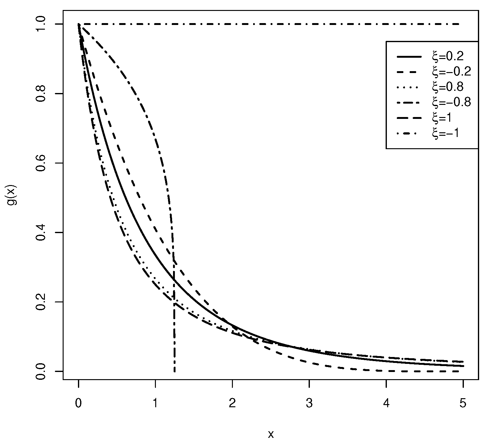
where , and are the shape, location, and scale parameters, respectively, and is the tail index. When , the three-parameter GPD reduces to the two-parameter GPD (, ). When , the domain of x is () and is heavy-tailed. When , , it is short-tailed. When , the GPD is a medium-tailed exponential distribution (more details can be found in [16]).
The corresponding probability density function (pdf) is
In order to show the flexibility and asymmetry of the GPD, we plot the pdfs of the GPD with various shape parameters in Figure 1.
The quantile function, , is
2.2. Peaks over Threshold (POT)
The EVT mainly studies the tail distribution characteristics of the continuous r.v. X, that is, the tail of , , and is also called the survival function [29]. If
we say that changes regularly varying with index or . When , is said to be slowly varying [17]. Based on this definition, there is a distribution that changes regularly as ∼, where is slowly varying. It is known that ∼ means . It can be concluded that the tail of a regularly varying distribution can be expressed by multiplying a slowly varying function by a power function. At this point, the distribution is called the maximum domain of attraction of the Fréchet distribution (, where ), representing a distribution class with heavy tails if and only if , where . The GPD is in [17].
The Pickands–Balkema–de Haan theorem (see [4,29]) states that, for , the excess loss from such a distribution with a high threshold converges to the GPD with Pareto parameter and . That is,
where , and is the right endpoint of F. This means that the excess distribution converges to the GPD when F is a heavy-tailed distribution in (see [4,29]).
It is worth noting that the GPD is stable with respect to excess over threshold operations [30]. This means that, if GPD(, ), the r.v. will follow the GPD (, ), where u is a threshold. This can also be derived for any that follows a parameter of of the GPD. This characteristic of the GPD illustrates that the excess above a threshold does not change the GPD shape parameter , but the GPD scale parameter is altered.
2.3. Value at Risk (VaR)
VaR reflects the maximum possible loss of the value of a financial dataset or portfolio of securities within a future time period, under a given probability level. Let be the distribution function of the population X; then, the p quantile of is , denoted by . The exceedance distribution above the threshold u can be defined by [30]
which is assumed to be . Therefore, can be expressed as
Based on the estimated parameters,
where is the EDF, and and are the estimations of the GPD parameters using the exceedances over the threshold. Then, the estimated p quantile of is
where n is the total sample size of observations, and is the number of observations lower than the threshold u.
3. Parameter Estimation Method
3.1. Existing Method GPWME
Chen et al. [18] proposed the population GPWME, and defined as follows
where both r and s are real numbers, and is a Borel measurable function for a parameter. Accordingly, the sample generalized probability weighted quasi-moment is defined as [18]
For convenience, note that X∼ represents the excess threshold data, and the corresponding represents the distribution function of the GPD. Denote as a random sample of size n from and denote as order statistics. Chen et al. [18] set , , , . The population GPWMEs are
For the sample, when,
Notice that
3.2. New Methods
3.2.1. GWNLSM Estimation
GPWME applies parameter estimation where the distribution is ideal. That is, in practice, for all observations, the specific distribution is unknown in advance. It is known that, based on the Pickands–Balkema–de Haan theorem, the tail region of the observations can be modeled via the GPD. Therefore, a parameter estimate of the GPD is required. We propose an improvement on the method by combining it with the WNLS proposed by Park and Kim [17]. Therefore, generalized weighted nonlinear least squares moment (GWNLSM) estimation is proposed within the POT framework.
For the threshold u, data less than the threshold are recorded as 0, and for data greater than the threshold, the exceedance is defined as . In order to obtain more accurate parameter estimates, the combination of the nonlinear least squares method and moment estimation is considered based on the GPWME method. The specific method is as follows.
Set
Within the POT framework, is replaced by Equation (2), and is replaced by . Using Equations (4) and (5), we have
where , , . The specific calculation process is shown in the Appendix A. For the sample moments, we have
In the first step, the interim estimator can be obtained via nonlinear minimization:
The following second step with as initial values and the third step with as initial values lead to another optimization:
Based on the idea of weighted least squares regression, we find that the performance of the third step estimation can be further improved by adding suitable weights in Equation (15). Set the weight to =(Var, where Var A revised version of the given nonlinear optimization is produced by adding weights:
Note that ; we modify as to smooth the error of VaR via numerous simulations. Combined with Equations (13), (14) and (16), the GWNLSM was proposed. One advantage of the proposed GWNLSM over the GPWME is that it obtains a more stable extreme quantile estimator. The effect of the error is reduced because each squared deviation term is multiplied by the corresponding weight. The standard “optim” function in R is used to implement the GWNLSM estimator in our numerical studies.Without a loss of generality, we take all starting values as in the following simulation and application. When , the GPD is heavy-tailed. The proposed estimated method is only applicable to the statistical inference of the heavy-tailed GPD.
3.2.2. Estimation
Based on the GWNLSM method, the values of and are calculated via a large number of simulations. With and fixed within a selection of ranges (−2, 2) and (0, 2), and a step size of 0.05, and have a total of 3280 pairs of combinations. A total of 3280 synthetic samples were employed to evaluate the root-mean-square error (RMSE) for of the fixed , p, and values. The values of range from 0.1 to 0.9, the values of p are 0.999 and 0.9999 and those of are 0.98, 0.99 and 0.995, where .
First, for a given , p and , count the minimum and maximum values of the RMSE for corresponding to each set of parameters and then change the values of u and p, in turn, to calculate the corresponding RMSE values. Taking as an example, because the values of u and p are different, there are seven combinations, based on the different values of and , a total of seven sets of RMSEs are calculated. Specifically, when is 0.98, p takes 0.99, 0.999, and 0.9999; when is 0.99, p takes 0.999 and 0.9999; and when is 0.995, p takes 0.999 and 0.9999. The results are shown in Table 1.
Table 1 shows the different values of , p, and , as well as the corresponding actual number of samples used. The values in the table are estimated via the corresponding and values; then, the corresponding RMSE values are obtained, where min and max represent the minimum and maximum values of RMSE, respectively.
Second, for the given and p, fix as a certain value, and sort the RMSE values from smallest to largest, selecting the top 5% values and their corresponding and . For these and , they are weighted and averaged, with the weight being the reciprocal of the corresponding RMSE divided by the reciprocal sum of the RMSE. Taking = 0.1 as an example, first sort the RMSE calculated by = 0.98 and p = 0.99 and select the first 5% of the lower RMSE values and their corresponding and . Based on the selected RMSE value, the weighted averages of and are carried out to obtain the final weighted and values. The weights of and are the reciprocal of their corresponding RMSE divided by the reciprocal of the previous 5% RMSE. At this point, the and values corresponding to = 0.1, and the = 0.98 and p = 0.99 can be calculated. Following the above steps, the and values corresponding to = 0.98, p = 0.999 and p = 0.9999 can also be calculated. This is the result based on classification when = 0.1. Similarly, we can obtain the result by fixing p as a certain value. By repeating the above steps, we can find the optimal values for and .
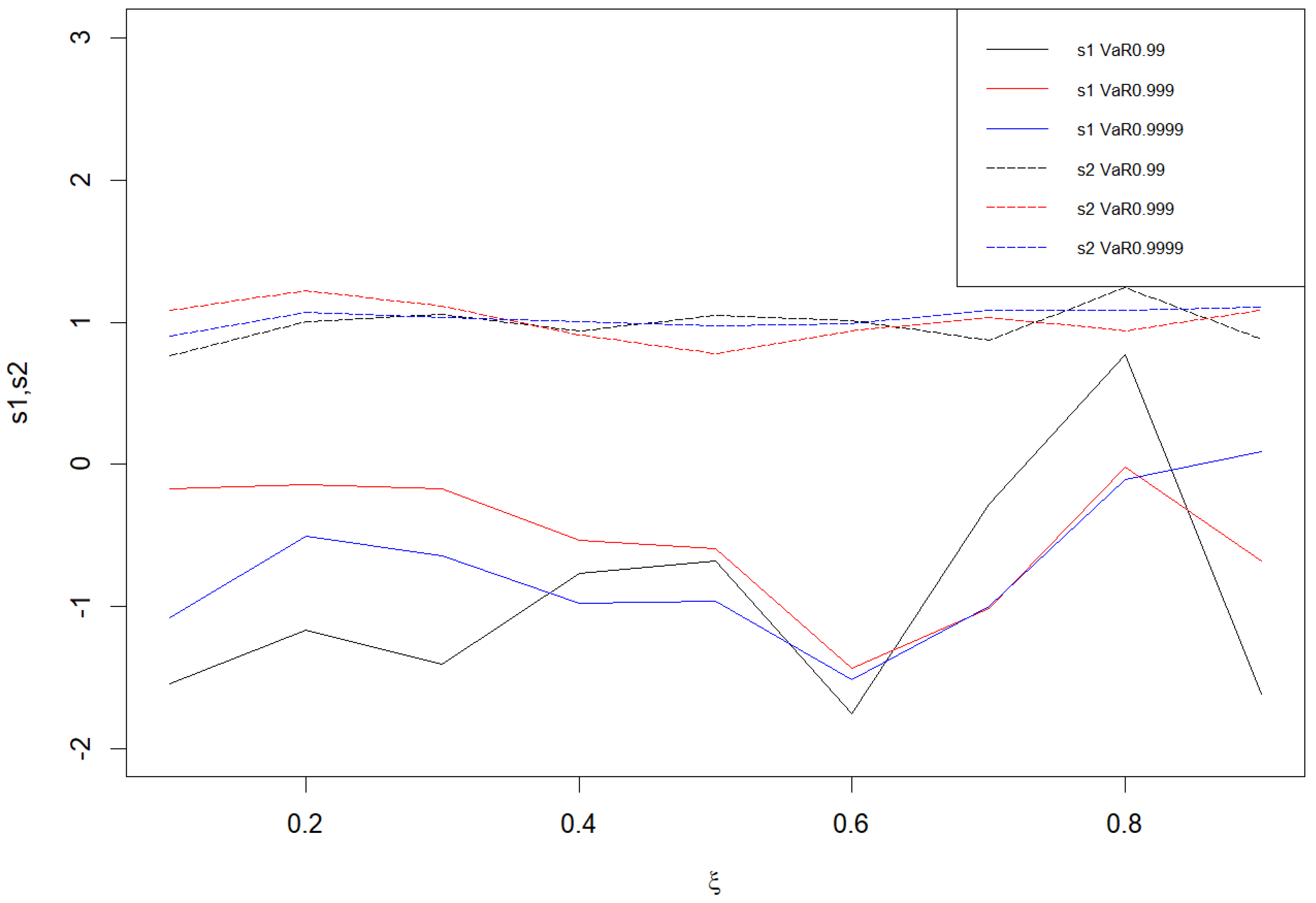
Third, the values of and based on fixing significantly fluctuate through calculation and comparison. Thus, the results of and based on fixing p are considered. Figure 2 is plotted in accordance with the p score, in which the upper three solid lines represent the image of , the lower three dashed lines represent the image of , and the different colored lines represent different values of p corresponding to . From the image, it can be observed that the value of fluctuates very little and the basic value of is around 1, while the basic value of is negative and the change fluctuation is relatively large. Based on the above analysis, = 1 and are used to find the function relationship. According to the results of and shown in Figure 2, we can establish a linear regression model for via the “lm” function in R. Through a regression analysis of the value and , the following model is obtained:
Equation (17) first requires using the existing method to estimate , and then determining according to the different p and values; it is relatively troublesome to determine . Therefore, RMSE is sorted from small to large. We select the first 30% of the data and their corresponding and value ranges, for a given p and ; and then selects to take the intersection of the value range of when taking different values, as the recommended value of , that is, . In the following simulation and application, the presented GWNLSM uses and for estimation parameters.
4. Simulation Studies
We only choose heavy-tailed distributions since our main interest is heavy-tailed data. The performance of the proposed methods is investigated via Monte Carlo simulations. The competing estimators in clude the LME estimator by Zhang [14], the WNLS by Park and Kim [17], the GPWME by Chen et al. [18], and our GWNLSM method. In addition, besides the GPD simulated samples, we also generate samples from the Cauchy and Pareto distribution. The purpose is to evaluate the robustness of the proposed method when the population distribution is misjudged. Our focus is on estimating VaR rather than the GPD parameter itself; thus, the parameter estimation results are not shown. The 98th, 99th, and 99.5th sample quantiles are selected as the thresholds u for each sample, and the estimated extreme quantiles are VaR at 99%, 99.9%, and 99.99%, respectively. We summarize the simulation procedure as follows:
- (1)
- Generate a sample from the given distribution, where the sample size is 10,000.
- (2)
- Given , then .
- (3)
- Estimate the parameters (, ) and the VaR (given in Equation (3)).
- (4)
- Repeat steps (1)–(3) 2000 times.
- (5)
- Compute the RMSE and the absolute relative bias (ARB) of each VaR estimator.
Note that there are 50–200 observations with different thresholds for the GPD fit, with a total sample size of 10,000.
It can be seen that there is a reasonable number of exceedances for researching extreme tails. Table 2 and Table 3 show the simulation results. Table 2 is based on the simulation data generated via the GPD, using different estimation methods to estimate VaR and calculate the corresponding index values. Table 3 uses the simulation data generated from the Cauchy distribution and Pareto distribution to estimate VaR. To highlight the objective under the condition of satisfying heavy-tailed distribution characteristics, our method proves to be effective even when the specific distribution form is incorrectly determined.
Example 1.
GPD() with different ξ values and .
As can be seen from Table 2, by comparison, the LME and WNLS perform better for estimating VaR at 99% in terms of RMSE and ARB. However, with an increasing p in the estimated quantile, the proposed GWNLSM’s performance improves. Overall, the GWNLSM is relatively stable. In all cases of estimation for VaR at 99.99%, the GWNLSM outperforms all other estimators in terms of the RMSE, regardless of the used threshold value. Notably, it can be seen that when is relatively small, the LME estimate is relatively accurate. As increases, the GWNLSM estimation error decreases, resulting in more accurate estimates compared to the other methods in most cases, as assessed via RMSE and ARB. In addition, as the threshold increases, the GWNLSM exhibits a smaller ARB for VaR at 99.99% compared to the other methods.
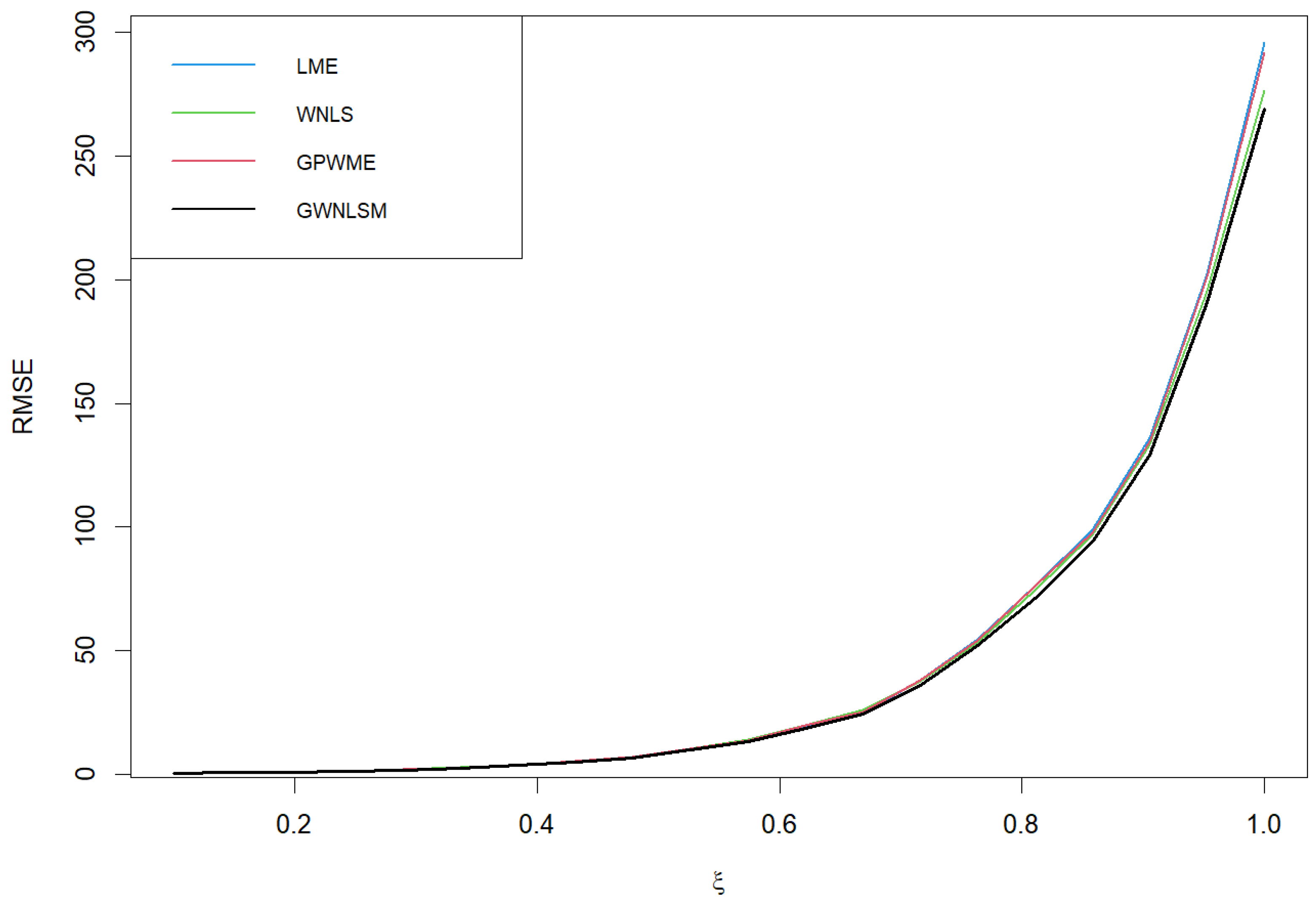
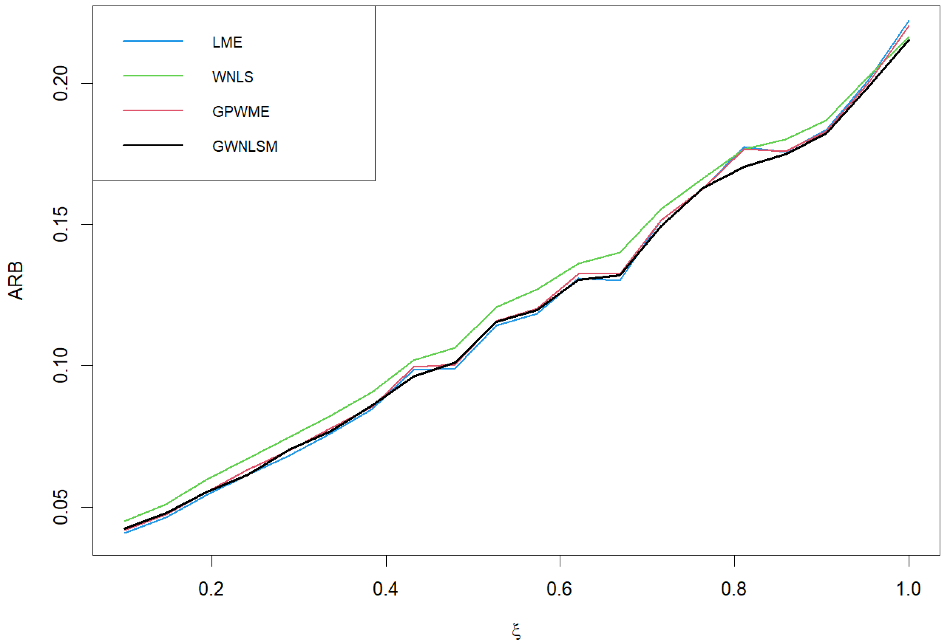
In order to facilitate the comparison and illustrate the effect of method improvement, we use = 0.995, p = 0.9999, and p = 0.999 as examples to draw comparisons, as shown in Figure 3, Figure 4, Figure 5, Figure 6, Figure 7 and Figure 8. The abscissa of Figure 3, Figure 4, Figure 5, Figure 6, Figure 7 and Figure 8 is the value of , where the ordinates in Figure 3, Figure 4, Figure 6 and Figure 7 represent the RMSE of VaR and the ordinates in Figure 5 and Figure 8 represent the ARB of VaR. We generate 10,000 samples from the GPD with and ranging from 0.1 to 1. This process is repeated 2000 times to calculate the RMSE and ARB of VaR at 99.99% and 99.9%. In terms of the RMSE and ARB of VaR at 99.99% and 99.9%, to better illustrate the advantages of the different estimation methods and show a discernible difference among curves in Figure 3 and Figure 6, we provide Figure 4 and Figure 7 as exploded views of Figure 3 and Figure 6, respectively. Here, in order to save space, we have only drawn a partial trend chart. In Figure 3, Figure 4, Figure 5, Figure 6, Figure 7 and Figure 8, we can see that the GWNLSM method performs better overall. For the RMSE evaluation criteria, GWNLSM estimation performed well in most cases. In terms of the ARB evaluation criteria, when is lower, the LME estimates VaR more accurately, and when is larger, the GWNLSM estimates VaR more accurately.
Example 2.
Cauchy (μ, σ). The cdf of the Cauchy distribution is defined as
where μ and σ are location and scale parameters.
We generated samples from the standard Cauchy distribution (, ) and presented the results in Table 3 with different thresholds. Table 3 illustrates that the GWNLSM outperforms other methods at 99.9% and 99.99% in terms of the RMSE and ARB with the 99th and 99.5th sample quantiles as thresholds.
Example 3.
Pareto ().
The cdf of the Pareto (type I) distribution is given by
where μ, σ, and α are the location, scale, and shape parameters.
The Pareto distribution is also another heavy-tailed distribution. We generated Pareto samples with and , and the results are presented in Table 3. As can be seen in Table 3, in most cases, our proposed method performs best again.
As can be seen from Table 3, for the Cauchy and the Pareto distributions, the GWNLSM parameter estimation method performs relatively well, regardless of a high- or low-threshold u, and the accuracy requirements of the estimated VaR are evidently superior. The higher the accuracy of the estimate, the more obvious the contrast error of various methods appears, and it is evident that the GWNLSM methods exhibit superiority over the LME, WNLS and GPWME methods in terms of performance. Whether it is a Cauchy or Pareto distribution, GWNLSM is optimal in most cases for VaR at 99.9% and VaR at 99.99%.
5. Actual Data Processing and Analysis
To verify the performance of different estimators, we chose PM2.5 data for our experimental analysis. PM2.5 data were obtained from the China National Environmental Monitoring Center. The center is a national technical institution and is directly affiliated with the Ministry of Ecology and Environment. It operates as the center of technology, network, information, quality control, and training for national environmental monitoring. In addition, it collects at least 100 million environmental monitoring data annually, which provides a strong guarantee for scientifically and accurately assessing national environmental quality. The PM2.5 monitoring results are also published online (https://www.cnemc.cn/ (accessed on 19
February 2023) We use the Beijing PM2.5 dataset from 2015 to 2022. The sample size is 2737. In order to preserve the original nature of the data and reduce the influence of scale parameter of the GPD, making it as small as possible, we changed the data separately, with the PM2.5 dataset reduced to 1% of the original. The following results are calculated based on transformed data.
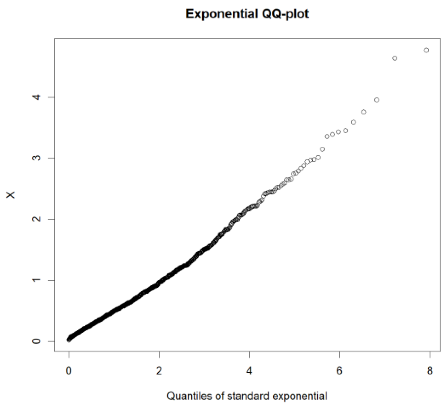
We select the threshold and the corresponding analysis calculation using the following steps. First, when the exponential QQ plot is convex, indicating that the empirical quantile is growing faster than the theoretical quantile, the distribution is heavy-tailed. Conversely, the explanation is a short-tailed distribution. The tail distribution characteristics of PM2.5 are examined. The exponential QQ plot is given in Figure 9. It is worth noting that, in the exponential QQ plot of this study, the x axes are theoretical quantiles, and the y axes are empirical quantiles. Contrary to the aforementioned theory QQ, Figure 9 shows a concave shape; it can be observed that the data used are subject to a heavy-tailed distribution.
For the heavy-tailed features of the diagnostic data, we also plotted the empirical mean excess function (EMEF), given in Figure 10. In general, if EMEF has a significant linear change after exceeding a certain threshold and the slope is positive, it indicates that the excess threshold data follow the GPD and the shape parameter is greater than 0. For heavy-tailed data, this threshold can be selected as the threshold for analysis; if EMEF has a significant linear change after a certain threshold, but the slope is negative, it indicates that the observed data are short-tailed. As can be seen from Figure 10, the dataset satisfied the heavy-tailed distribution.
Secondly, a suitable threshold is selected. The preliminary value of the threshold can be roughly observed in the mean residual life plot. Another way to initially select a threshold is through the Hill plot in Figure 10. The trend stabilization point of the Hill plot is generally determined as a threshold. By observing the EMEF and Hill plots in Figure 10, it can be intuitively judged that the u value is about 1.
In order to find a more suitable and objective threshold u, we use goodness-of-fit tests to select the threshold. The main objective is to find the lowest threshold such that the highest number of exceedances above the threshold follows the GPD. We use the AD test statistic [22].
The details of the threshold selection method, instance calculation, and simulation steps are as follows.
- (1)
- Threshold selection. For the PM2.5 data, we combine the AD statistic and the Raw Down method to select the threshold , exceeding the number , , where Raw Down means that the test begins at the largest threshold and choose the first threshold until the test is rejected, then the threshold before the rejection is chosen [24].
- (2)
- (3)
- Based on the above parameter estimation results, random samples following GPD and , , are calculated.
- (4)
- Repeat (3) 1000 times; RMSE and ARB for VaR are calculated. Some results are shown in Table 5.
Table 5 compares the index values of the VaR based on four parameter estimation methods for the PM2.5 data. From Table 5, we can see that the LME and proposed GWNLSM exhibit better performances for VaR at 99.9% and VaR at 99.99% in terms of RMSE and ARB. Specifically, it can be observed that the proposed method works better for VaR at 99.99% in most cases.
6. Conclusions
In this study, based on the GPWME method within the POT framework, we present a novel GPD parameter estimation GWNLSM. The proposed method is applicable to the heavy-tailed GPD when the shape parameter is greater than 0. This method utilizes the concepts of nonlinear least squares estimation and moment estimation while applying GPWME to the POT framework. In terms of the RMSE and ARB, extensive simulation studies and real-world datasets have shown that the advantage of the newly proposed estimator when VaRs are at high confidence levels. For example, when the estimated extreme quantile VaR is 99.99%, GWNLSM is optimal in most cases. Furthermore, when a set of data satisfies other heavy-tailed distributions, we can still use the asymmetrical GPD to obtain approximate extreme quantile estimates. The resulting extreme quantile estimates also exhibit relatively small errors. The new method performs well for heavy-tailed Cauchy and Pareto distributions and the actual dataset we present. A future research direction involves exploring more accurate and simpler methods to estimate the GPD parameters within the POT framework and optimizing the selection of and .
Author Contributions
Formal analysis, W.C. (Wenru Chen) and X.Z.; funding acquisition, X.Z., H.C., Q.J. and W.C. (Weihu Cheng); supervision, X.Z., H.C. and W.C. (Weihu Cheng); validation, X.Z., H.C. and W.C. (Weihu Cheng); writing—original draft, W.C. (Wenru Chen), X.Z., M.Z. and Q.J.; writing—review and editing, W.C. (Wenru Chen) and X.Z. All authors have read and agreed to the published version of the manuscript.
Funding
The authors would like to thank the National Office for Philosophy and Social Sciences (grant number: 20BTJ054) for their support.
Data Availability Statement
The data are published in https://www.cnemc.cn/ (accessed on 19 February 2023).
Acknowledgments
The authors would like to thank the referees and editors for their very helpful and constructive comments, which have significantly improved the quality of this paper.
Conflicts of Interest
The authors declare no conflicts of interest.
Appendix A
This section gives the calculation process of in detail.
Suppose that we have a sample of size n. For convenience, we write as, where follows . Hence, we have
and
Hence,
At the same time, we can also obtain the following results
Therefore,
and
References
- Tawn, J.A. Bivariate extreme value theory: Models and estimation. Biometrika 1988, 75, 397–415. [Google Scholar] [CrossRef]
- Tawn, J.A. Modelling multivariate extreme value distributions. Biometrika 1988, 77, 245–253. [Google Scholar] [CrossRef]
- Embrechts, P.; Resnick, S.I.; Gennady, S. Extreme Value Theory as a Risk Management Tool. N. Am. Actuar. J. 1999, 3, 30–41. [Google Scholar] [CrossRef]
- Pickands, J. Statistical inference using extreme order statistics. Ann. Stat. 1975, 3, 119–131. [Google Scholar]
- Hosking, J.R.; Wallis, J.R. Parameter and quantile estimation for the generalized pareto distribution. Technometrics 1987, 29, 339–349. [Google Scholar] [CrossRef]
- Greenwood, J.A.; Landwehr, J.M.; Matalas, N.C.; Wallis, J.R. Probability weighted moments: Definition and relation to parameters of several distributions expressable in inverse form. Water Resour. Res. 1979, 15, 1049–1054. [Google Scholar] [CrossRef]
- Smith, R.L. Maximum likelihood estimation in a class of nonregular cases. Biometrika 1985, 72, 67–90. [Google Scholar] [CrossRef]
- Moharram, S.; Gosain, A.; Kapoor, P. A comparative study for the estimators of the generalized pareto distribution. J. Hydrol. 1993, 150, 169–185. [Google Scholar] [CrossRef]
- Hosking, J.R. L-moments: Analysis and estimation of distributions using linear combinations of order statistics. J. R. Stat. Soc. Ser. B (Methodol.) 1990, 52, 105–124. [Google Scholar] [CrossRef]
- Ashkar, F.; Ouarda, T.B. On some methods of fitting the generalized pareto distributions. J. Hydrol. 1996, 177, 117–141. [Google Scholar] [CrossRef]
- Castillo, E.; Hadi, A.S. Fitting the generalized pareto distribution to data. J. Am. Stat. Assoc. 1997, 92, 1609–1620. [Google Scholar] [CrossRef]
- From, S.G.; Ratnasingam, S. Some efficient closed-form estimators of the parameters of the generalized pareto distribution. Environ. Ecol. Stat. 2022, 29, 827–847. [Google Scholar] [CrossRef]
- Rasmussen, P.F. Generalized probability weighted moments: Application to the generalized pareto distribution. Water Resour. Res. 2001, 37, 1745–1751. [Google Scholar] [CrossRef]
- Zhang, J. Likelihood moment estimation for the generalized pareto distribution. Aust. N. Z. J. Stat. 2007, 49, 69–77. [Google Scholar] [CrossRef]
- Zhang, J.; Stephens, M.A. A new and efficient estimation method for the generalized pareto distribution. Technometrics 2009, 51, 316–325. [Google Scholar] [CrossRef]
- Song, J.; Song, S. A quantile estimation for massive data with generalized pareto distribution. Comput. Stat. Data Anal. 2012, 56, 143–150. [Google Scholar] [CrossRef]
- Park, M.H.; Kim, J.H. Estimating extreme tail risk measures with generalized pareto distribution. Comput. Stat. Data Anal. 2016, 98, 91–104. [Google Scholar] [CrossRef]
- Chen, H.; Cheng, W.; Zhao, J.; Zhao, X. Parameter estimation for generalized Pareto distribution by generalized probability weighted moment-equations. Commun.-Stat.-Simul. Comput. 2017, 46, 7761–7776. [Google Scholar] [CrossRef]
- Chen, P.; Ye, Z.S.; Zhao, X. Minimum distance estimation for the generalized pareto distribution. Technometrics 2017, 59, 528–541. [Google Scholar] [CrossRef]
- Martín, J.; Parra, M.I.; Pizarro, M.M.; Sanjuán, E.L. Baseline methods for the parameter estimation of the generalized pareto distribution. Entropy 2022, 24, 178. [Google Scholar] [CrossRef] [PubMed]
- Langousis, A.; Mamalakis, A.; Puliga, M.; Deidda, R. Threshold detection for the generalized pareto distribution: Review of representative methods and application to the noaa ncdc daily rainfall database. Water Resour. Res. 2016, 52, 2659–2681. [Google Scholar] [CrossRef]
- Choulakian, V.; Stephens, M.A. Goodness-of-fit tests for the generalized pareto distribution. Technometricsh 2001, 43, 478–484. [Google Scholar] [CrossRef]
- G’Sell, M.G.; Wager, S.; Chouldechova, A. Sequential selection procedures and false discovery rate control. J. R. Stat. Ser. B Stat. Methodol. 2016, 78, 423–444. [Google Scholar] [CrossRef]
- Bader, B.; Yan, J.; Zhang, X. Automated threshold selection for extreme value analysis via ordered goodness-of-fit tests with adjustment for false discovery rate. Ann. Appl. Stat. 2018, 12, 310–329. [Google Scholar] [CrossRef]
- Yang, X.; Zhang, J.; Ren, W.X. Threshold selection for extreme value estimation of vehicle load effect on bridges. Int. J. Distrib. Sens. Netw. 2018, 14, 1–12. [Google Scholar] [CrossRef]
- Annabestani, M.; Saadatmand-Tarzjan, M. A new threshold selection method based on fuzzy expert systems for separating text from the background of document images. Iran. J. Sci. Technol. Trans. Electrical Eng. 2019, 43, 219–231. [Google Scholar] [CrossRef]
- Curceac, S.; Atkinson, P.M.; Milne, A.; Wu, L.; Harris, P. An evaluation of automated GPD threshold selection methods for hydrological extremes across different scales. J. Hydrol. 2020, 585, 124845. [Google Scholar] [CrossRef]
- Silva Lomba, J.; Fraga Alves, M.I. L-moments for automatic threshold selection in extreme value analysis. Stoch. Environ. Res. Risk Assess. 2020, 34, 465–491. [Google Scholar] [CrossRef]
- Balkema, A.A.; De Haan, L.I. Residual life time at great age. Ann. Probab. 1974, 2, 792–804. [Google Scholar] [CrossRef]
- De Zea Bermudez, P.; Kotz, S. Parameter estimation of the generalized Pareto distribution—Part I. J. Stat. Plan. Inference 2010, 140, 1353–1373. [Google Scholar] [CrossRef]
- Landwehr, J.M.; Matalas, N.; Wallis, J. Estimation of parameters and quantiles of wakeby distributions. Water Resour. Res. 1979, 15, 1361–1372. [Google Scholar] [CrossRef]
Figure 1.
pdfs of GPD.

Figure 2.
Plot of and with different values (solid and dashed lines represent values of and , respectively, while ).
Figure 2.
Plot of and with different values (solid and dashed lines represent values of and , respectively, while ).

Figure 3.
RMSE of VaR at 99.99% with and 98th quantile as threshold.

Figure 4.
RMSE of VaR at 99.99% with and 98th quantile as threshold (exploded view of Figure 3).
Figure 4.
RMSE of VaR at 99.99% with and 98th quantile as threshold (exploded view of Figure 3).

Figure 5.
ARB of VaR at 99.99% with and 98th quantile as the threshold.

Figure 6.
RMSE of VaR at 99.9% with and 98th quantile as threshold.

Figure 7.
RMSE of VaR at 99.9% with and 98th quantile as the threshold (exploded view of Figure 6).
Figure 7.
RMSE of VaR at 99.9% with and 98th quantile as the threshold (exploded view of Figure 6).

Figure 8.
ARB of VaR at 99.9% with and 98th quantile as threshold.

Figure 9.
The QQ diagram of the PM2.5 data; the ordinate x represents order data.

Figure 10.
The EMEF and Hill diagrams of the PM2.5 data. In (a), the black and grey lines represent the empirical mean residual life and its confidence intervals with confidence level 0.95. In (b), the black and blue lines represent the Hill estimator of the GPD tail index and its confidence intervals with confidence level 0.95.


Table 1.
and correspond to the RMSE values of , where and are used in (13) and (14).
| p = 0.99 | p = 0.999 | p = 0.9999 | ||||
|---|---|---|---|---|---|---|
| Min | Max | Min | Max | Min | Max | |
| ( = 0.98) | ||||||
| 0.1 | 0.1505 | 0.1507 | 0.5241 | 0.5245 | 1.8920 | 1.8943 |
| 0.2 | 0.2417 | 0.3880 | 1.0468 | 1.9865 | 4.5350 | 5.9320 |
| 0.3 | 0.3874 | 0.5727 | 2.0901 | 3.3288 | 10.931 | 12.778 |
| 0.4 | 0.6203 | 0.6342 | 4.1739 | 4.2635 | 26.574 | 26.820 |
| 0.5 | 0.9916 | 1.0179 | 8.3218 | 8.4833 | 64.592 | 65.264 |
| 0.6 | 1.5879 | 1.6469 | 16.629 | 17.084 | 160.04 | 161.07 |
| 0.7 | 2.5359 | 2.6193 | 33.193 | 33.911 | 386.40 | 398.62 |
| 0.8 | 4.0551 | 4.2626 | 66.226 | 68.616 | 987.72 | 1012.01 |
| 0.9 | 6.4608 | 6.8859 | 132.31 | 136.16 | 2489.05 | 2655.14 |
| ( = 0.99) | ||||||
| 0.1 | 0.5206 | 0.5465 | 2.0061 | 2.0466 | ||
| 0.2 | 1.0371 | 2.7049 | 4.8787 | 8.0178 | ||
| 0.3 | 2.0664 | 4.3109 | 11.912 | 16.020 | ||
| 0.4 | 4.1189 | 4.3153 | 29.4287 | 29.761 | ||
| 0.5 | 8.2235 | 8.6656 | 73.150 | 74.088 | ||
| 0.6 | 16.419 | 16.982 | 182.86 | 185.17 | ||
| 0.7 | 32.708 | 34.350 | 461.78 | 476.22 | ||
| 0.8 | 65.731 | 74.542 | 1184.33 | 1604.15 | ||
| 0.9 | 131.40 | 173.90 | 2853.84 | 3542.59 | ||
| ( = 0.995) | ||||||
| 0.1 | 0.5544 | 0.6366 | 2.0507 | 2.2331 | ||
| 0.2 | 1.1021 | 2.5829 | 5.0543 | 8.8306 | ||
| 0.3 | 2.1912 | 4.2018 | 12.534 | 17.377 | ||
| 0.4 | 4.3598 | 4.5966 | 31.228 | 31.827 | ||
| 0.5 | 8.6729 | 9.1764 | 78.282 | 81.745 | ||
| 0.6 | 17.156 | 19.610 | 198.75 | 216.080 | ||
| 0.7 | 34.499 | 48.666 | 508.52 | 548.680 | ||
| 0.8 | 68.833 | 125.12 | 1301.21 | 1548.14 | ||
| 0.9 | 137.790 | 293.19 | 3388.58 | 5448.34 | ||
Table 2.
RMSE and ARB are calculated for each VaR estimation from the GPD with different values.
| RMSE | ARB | ||||||
|---|---|---|---|---|---|---|---|
| VaR | VaR | VaR | VaR | VaR | VaR | ||
| GPD (0.2, 1) | |||||||
| = 0.98 | LME | 0.2358 | 1.0236 | 4.6917 | 0.0249 | 0.0548 | 0.1364 |
| WNLS | 0.2363 | 1.1068 | 5.1240 | 0.0250 | 0.0600 | 0.1528 | |
| GPWME | 0.2406 | 1.0464 | 5.1278 | 0.0255 | 0.0558 | 0.1459 | |
| GWNLSM | 0.2423 | 1.0412 | 4.5217 | 0.0253 | 0.0564 | 0.1388 | |
| = 0.99 | LME | 1.0274 | 5.2043 | 0.0550 | 0.1511 | ||
| WNLS | 1.0902 | 5.6780 | 0.0590 | 0.1715 | |||
| GPWME | 1.0388 | 5.9179 | 0.0555 | 0.1661 | |||
| GWNLSM | 1.0350 | 4.8295 | 0.0559 | 0.1484 | |||
| = 0.995 | LME | 1.0889 | 5.4096 | 0.0581 | 0.1559 | ||
| WNLS | 1.0973 | 5.6234 | 0.0592 | 0.1718 | |||
| GPWME | 1.0928 | 6.0105 | 0.0582 | 0.1675 | |||
| GWNLSM | 1.0959 | 5.0130 | 0.0589 | 0.1534 | |||
| GPD (0.4, 1) | |||||||
| = 0.98 | LME | 0.5960 | 4.1581 | 28.526 | 0.0359 | 0.0889 | 0.2208 |
| WNLS | 0.5963 | 4.3481 | 29.282 | 0.0359 | 0.0945 | 0.2346 | |
| GPWME | 0.6043 | 4.2111 | 30.011 | 0.0364 | 0.0897 | 0.2286 | |
| GWNLSM | 0.6210 | 4.1443 | 26.543 | 0.0369 | 0.0905 | 0.2209 | |
| = 0.99 | LME | 4.1749 | 33.105 | 0.0893 | 0.2527 | ||
| WNLS | 4.3218 | 33.957 | 0.0939 | 0.2705 | |||
| GPWME | 4.2194 | 36.377 | 0.0901 | 0.2708 | |||
| GWNLSM | 4.1020 | 29.095 | 0.0892 | 0.2411 | |||
| = 0.995 | LME | 4.3559 | 35.972 | 0.0927 | 0.2684 | ||
| WNLS | 4.3036 | 34.655 | 0.0935 | 0.2800 | |||
| GPWME | 4.3624 | 38.747 | 0.0928 | 0.2800 | |||
| GWNLSM | 4.3250 | 30.981 | 0.0932 | 0.2542 | |||
| GPD (0.8, 1) | |||||||
| = 0.98 | LME | 3.8021 | 68.581 | 1157.57 | 0.0624 | 0.1704 | 0.4027 |
| WNLS | 3.7820 | 67.292 | 1054.26 | 0.0623 | 0.1720 | 0.3890 | |
| GPWME | 3.8128 | 68.095 | 1142.27 | 0.0627 | 0.1690 | 0.3976 | |
| GWNLSM | 4.0488 | 65.579 | 989.23 | 0.0656 | 0.1697 | 0.3828 | |
| = 0.99 | LME | 69.805 | 1480.19 | 0.1732 | 0.4870 | ||
| WNLS | 68.472 | 1349.27 | 0.1753 | 0.4726 | |||
| GPWME | 70.129 | 1520.94 | 0.1739 | 0.4998 | |||
| GWNLSM | 65.032 | 1155.32 | 0.1674 | 0.4314 | |||
| = 0.995 | LME | 71.113 | 1812.26 | 0.1758 | 0.5483 | ||
| WNLS | 67.375 | 1436.30 | 0.1726 | 0.5027 | |||
| GPWME | 71.083 | 1799.72 | 0.1758 | 0.4694 | |||
| GWNLSM | 67.983 | 1292.96 | 0.1720 | 0.4694 | |||
| GPD (2, 1) | |||||||
| = 0.98 | LME | 981.834 | 3.28 | 1.32 | 0.1535 | 0.4490 | 1.1581 |
| WNLS | 958.756 | 2.78 | 8.93 | 0.1511 | 0.4028 | 0.8835 | |
| GPWME | 961.981 | 3.11 | 1.11 | 0.1508 | 0.4311 | 1.0458 | |
| GWNLSM | 3257.37 | 4.49 | 5.82 | 0.5939 | 0.8414 | 0.9610 | |
| = 0.99 | LME | 3.58 | 2.65 | 0.4786 | 1.72649 | ||
| WNLS | 3.02 | 1.56 | 0.4339 | 1.2574 | |||
| GPWME | 3.57 | 2.29 | 0.4793 | 1.6624 | |||
| GWNLSM | 4.89 | 5.23 | 0.9684 | 1.0007 | |||
| = 0.995 | LME | 3.59 | 6.07 | 0.4777 | 2.5958 | ||
| WNLS | 2.96 | 2.45 | 0.4268 | 1.5203 | |||
| GPWME | 4.26 | 7.44 | 0.5410 | 4.5462 | |||
| GWNLSM | 4.79 | 4.99 | 0.9568 | 0.9976 | |||
Table 3.
RMSE and ARB for different heavy-tailed distributions.
| RMSE | ARB | ||||||
|---|---|---|---|---|---|---|---|
| VaR | VaR | VaR | VaR | VaR | VaR | ||
| Cauchy (0, 1) | |||||||
| = 0.98 | LME | 3.1092 | 88.443 | 2318.32 | 0.0775 | 0.2120 | 0.4773 |
| WNLS | 3.0863 | 85.680 | 2033.446 | 0.0772 | 0.2121 | 0.4527 | |
| GPWME | 3.0866 | 87.650 | 2230.66 | 0.0770 | 0.2095 | 0.4681 | |
| GWNLSM | 3.3829 | 82.235 | 1949.25 | 0.0839 | 0.2078 | 0.4417 | |
| = 0.99 | LME | 90.650 | 3202.64 | 0.2166 | 0.5904 | ||
| WNLS | 85.880 | 2707.33 | 0.2138 | 0.5293 | |||
| GPWME | 90.269 | 3123.24 | 0.2158 | 0.5799 | |||
| GWNLSM | 82.370 | 2462.95 | 0.2066 | 0.5153 | |||
| = 0.995 | LME | 91.416 | 4325.15 | 0.2178 | 0.7113 | ||
| WNLS | 84.334 | 3070.36 | 0.2111 | 0.5997 | |||
| GPWME | 91.209 | 4022.12 | 0.2175 | 0.6959 | |||
| GWNLSM | 85.447 | 3379.91 | 0.2106 | 0.5925 | |||
| Pareto (1, 1) | |||||||
| = 0.98 | LME | 9.3271 | 280.801 | 7496.16 | 0.0756 | 0.21743 | 0.5073 |
| WNLS | 9.3032 | 270.150 | 6702.71 | 0.0754 | 0.21501 | 0.4791 | |
| GPWME | 9.3260 | 278.776 | 7322.52 | 0.0755 | 0.2163 | 0.5041 | |
| GWNLSM | 10.079 | 263.021 | 6286.66 | 0.0814 | 0.2126 | 0.4683 | |
| = 0.99 | LME | 286.769 | 9886.04 | 0.2208 | 0.6097 | ||
| WNLS | 271.847 | 8537.50 | 0.2168 | 0.5585 | |||
| GPWME | 286.754 | 9904.80 | 0.22084 | 0.6094 | |||
| GWNLSM | 262.670 | 7461.39 | 0.2110 | 0.5345 | |||
| = 0.995 | LME | 287.946 | 14914.1 | 0.2212 | 0.7202 | ||
| WNLS | 265.757 | 10433.2 | 0.2133 | 0.6269 | |||
| GPWME | 287.636 | 13634.9 | 0.2210 | 0.7170 | |||
| GWNLSM | 274.081 | 9534.50 | 0.2161 | 0.6060 | |||
Table 4.
Parameter estimation for real data using different methods.
| LME | 0.0782 | 0.5185 |
| WNLS | 0.1169 | 0.4953 |
| GPWME | 0.0813 | 0.5169 |
| GWNLSM | 0.0481 | 0.5363 |
| u | 0.83 | |
Table 5.
VaR estimation of the PM2.5 data.
| RMSE | ARB | |||||
|---|---|---|---|---|---|---|
| VaR at | VaR at | VaR at | VaR at | VaR at | VaR at | |
| LME | ||||||
| LME | 0.939642 | 3.567475 | 9.359341 | 0.029951 | 0.069050 | 0.140593 |
| WNLS | 1.114730 | 4.347896 | 11.12457 | 0.049561 | 0.102806 | 0.165263 |
| GPWME | 1.033365 | 4.195512 | 11.23957 | 0.045660 | 0.096672 | 0.161397 |
| GWNLSM | 1.021122 | 3.781147 | 9.356901 | 0.045634 | 0.083634 | 0.140933 |
| WNLS | ||||||
| LME | 1.068671 | 4.288407 | 11.87006 | 0.032968 | 0.077429 | 0.136665 |
| WNLS | 1.194244 | 4.963725 | 13.53752 | 0.037138 | 0.091490 | 0.159159 |
| GPWME | 1.110651 | 4.800949 | 13.69599 | 0.034303 | 0.086194 | 0.155536 |
| GWNLSM | 1.097004 | 4.361997 | 11.53057 | 0.034309 | 0.080041 | 0.136313 |
| GPWME | ||||||
| LME | 0.729066 | 2.94535 | 8.193269 | 0.025959 | 0.061376 | 0.1145927 |
| WNLS | 0.787671 | 3.432898 | 9.433241 | 0.028197 | 0.072860 | 0.132312 |
| GPWME | 0.739436 | 3.287148 | 9.479313 | 0.026414 | 0.068239 | 0.128704 |
| GWNLSM | 0.745556 | 3.017241 | 8.055831 | 0.026776 | 0.064257 | 0.114585 |
| GWNLSM | ||||||
| LME | 1.596907 | 4.875529 | 10.94257 | 0.041240 | 0.083499 | 0.134014 |
| WNLS | 1.889057 | 5.813446 | 12.88081 | 0.049464 | 0.101360 | 0.160320 |
| GPWME | 1.739965 | 5.616292 | 12.95679 | 0.045003 | 0.095299 | 0.155665 |
| GWNLSM | 1.651400 | 4.856433 | 10.34925 | 0.043370 | 0.083253 | 0.132417 |
Disclaimer/Publisher’s Note: The statements, opinions and data contained in all publications are solely those of the individual author(s) and contributor(s) and not of MDPI and/or the editor(s). MDPI and/or the editor(s) disclaim responsibility for any injury to people or property resulting from any ideas, methods, instructions or products referred to in the content. |
© 2024 by the authors. Licensee MDPI, Basel, Switzerland. This article is an open access article distributed under the terms and conditions of the Creative Commons Attribution (CC BY) license (https://creativecommons.org/licenses/by/4.0/).
Share and Cite
MDPI and ACS Style
Chen, W.; Zhao, X.; Zhou, M.; Chen, H.; Ji, Q.; Cheng, W. Statistical Inference and Application of Asymmetrical Generalized Pareto Distribution Based on Peaks-Over-Threshold Model. Symmetry 2024, 16, 365. https://doi.org/10.3390/sym16030365
AMA Style
Chen W, Zhao X, Zhou M, Chen H, Ji Q, Cheng W. Statistical Inference and Application of Asymmetrical Generalized Pareto Distribution Based on Peaks-Over-Threshold Model. Symmetry. 2024; 16(3):365. https://doi.org/10.3390/sym16030365
Chicago/Turabian StyleChen, Wenru, Xu Zhao, Mi Zhou, Haiqing Chen, Qingqing Ji, and Weihu Cheng. 2024. "Statistical Inference and Application of Asymmetrical Generalized Pareto Distribution Based on Peaks-Over-Threshold Model" Symmetry 16, no. 3: 365. https://doi.org/10.3390/sym16030365
Note that from the first issue of 2016, this journal uses article numbers instead of page numbers. See further details here.