Efficient Multistep Algorithms for First-Order IVPs with Oscillating Solutions: II Implicit and Predictor–Corrector Algorithms

Abstract

This research introduces a fresh methodology for creating efficient numerical algorithms to solve first-order Initial Value Problems (IVPs). The study delves into the theoretical foundations of these methods and demonstrates their application to the Adams–Moulton technique in a five-step process. We focus on developing amplification-fitted algorithms with minimal phase-lagor phase-lag equal to zero (phase-fitted). The request of amplification-fitted (zero dissipation) is to ensure behavior like symmetric multistep methods (symmetric multistep methods are methods with zero dissipation). Additionally, the stability of the innovative algorithms is examined. Comparisons between our new algorithm and traditional methods reveal its superior performance. Numerical tests corroborate that our approach is considerably more effective than standard methods for solving IVPs, especially those with oscillatory solutions.

1. Introduction

Equations or systems of Equations of the form

$${\mathbf{s}}^{\prime }\left(\mathbf{t}\right)=\mathbf{q}(\mathbf{t},\mathbf{s}),\mathbf{s}\left({\mathbf{t}}_{\mathbf{0}}\right)={\mathbf{s}}_{\mathbf{0}}$$

(1)

are utilized across a range of fields such as astrophysics, chemistry, physics, electronics, nanotechnology, materials science, and more. Equations with oscillatory or periodic solutions are of particular interest (refer to [1,2]).

Extensive research has been dedicated to studying the numerical solutions for the aforementioned equation or system of equations over the past two decades (see, for instance [3,4,5,6,7,8,9,10,11], and references therein). For a detailed examination of techniques for solving (1) with oscillating solutions, refer to [3,7,12], as well as the works of Quinlan and Tremaine [5,6,8,13], among others. Most existing numerical methods for solving (1) share a common feature of being multistep or hybrid approaches and were primarily developed for second-order differential equations. Some of the key method categories and their bibliography include:

• Exponentially-fitted, Trigonometrically-Fitted, Phase-Fitted, and Amplification-Fitted Runge–Kutta and Runge–Kutta-Nyström Methods with minimal phase-lag (refer to [14,15,16,17,18,19,20,21,22,23,24,25,26,27,28,29,30,31,32,33,34,35,36,37,38,39,40,41,42,43,44,45,46,47,48,49]);
• Exponentially-fitted and Trigonometrically-Fitted Phase-Fitted and Amplification-Fitted Multistep Methods and Multistep Methods with minimal phase-lag (refer to [50,51,52,53,54,55,56,57,58,59,60,61,62,63,64,65,66,67,68,69,70,71,72,73,74,75,76,77,78,79,80,81,82,83,84,85,86,87,88,89,90,91,92,93,94,95,96,97,98,99,100,101,102,103,104,105,106,107,108,109,110,111,112,113,114]).

Recently, Simos [115] developed the theory for the development of multistep methods with minimal phase-lag or phase-fitted multistep methods for first-order IVPs. More specifically, he developed the theory for computing the phase-lag and amplification error of multistep methods for first-order IVPs. In this paper, we will extend this theory to the implicit multistep methods for first-order IVPs This paper introduces the theory.

The rest of the paper is structured as follows:

• Section 2 presents the general theory for calculating the phase-lag and amplification error of implicit multistep methods for first-order IVPs. In this section, we produce the direct formulae for the calculation of the phase-lag and amplification factor;
• Section 3 introduces the methodologies and the methods which that will be developed in Section 4, Section 5, Section 6, Section 7, Section 8, Section 9, Section 10, Section 11, Section 12, Section 13 and Section 14. In this section, we present the methodologies for the development of efficient multistep methods for first-order initial value problems;
• Section 4 introduces the Adams–Bashforth five-step method and presents the methodology for the minimization of the phase-lag. In this section, we present the explicit Adams–Bashforth five-step method and we study its phase-lag and amplification error.;
• Section 5 presents the development of the amplification-fitted Adams–Bashforth five-step method of fourth algebraic order with phase-lag of order four. Based on the theory developed in Section 2, we eliminate the amplification error and we calculate the coefficients of the method in order for the method to have phase-lag of order four;
• Section 6 presents the development of the amplification-fitted Adams–Bashforth five-step method of third algebraic order with phase-lag of order six. Based on the theory presented in Section 2, we eliminate the amplification error and we calculate the coefficients of the method in order for the method to have phase-lag of order six.
• Section 7 presents the development of the amplification-fitted Adams–Bashforth five-step method of fourth algebraic order. We calculate the coefficients of the method, in order for its amplification error to be equal to zero;
• Section 8 presents the development of the amplification-fitted and phase-fitted Adams–Bashforth five-step method of fourth algebraic order. We calculate the coefficients of the method, in order for its phase-lag and amplification error to be eliminated;
• Section 9 introduces the Adams–Moulton five-step method and presents the methodology for the minimization of the phase-lag. In this section, we present the implicit Adams–Moulton five-step method and we study its phase-lag and amplification error;
• Section 10 presents the development of the amplification-fitted Adams–Moulton five-step method of fifth algebraic order with phase-lag of order four. Based on the theory developed in Section 2, we eliminate the amplification error and we calculate the coefficients of the method in order for the method to have phase-lag of order four;
• Section 11 presents the development of the amplification-fitted Adams–Moulton five-step method of second algebraic order with phase-lag of order six. Based on the theory presented in Section 2, we vanish the amplification error and we calculate the coefficients of the method in order for the method to have phase-lag of order six;
• Section 12 presents the development of the amplification-fitted Adams–Moulton five-step method of second algebraic order with phase-lag of order eight. Based on the theory presented in Section 2, we demand the amplification error to be equal to zero and we calculate the coefficients of the method in order for the method to have phase-lag of order eight;
• Section 13 presents the development of the amplification-fitted Adams–Moulton five-step method of fifth algebraic order.We calculate the coefficients of the method, in order for its amplification error to be equal to zero;
• Section 14 presents the development of the amplification-fitted and phase-fitted Adams–Moulton five-step method of fifth algebraic order. We calculate the coefficients of the method, in order for its phase-lag and amplification error to be eliminated;
• Section 15 discusses a stability analysis for the newly proposed methods in Section 4, Section 5, Section 6, Section 7, Section 8, Section 9, Section 10, Section 11, Section 12, Section 13 and Section 14. We examine the stability of the developed methods for several values of v.
• Section 16 presents numerical results. We examine the efficiency of the proposed methods in their application on seven well-known problems. For each problem, we give conclusion for the behavior of the developed methods;
• Finally, Section 17 presents the conclusions of this research.

The numerical results demonstrate that the methodology for developing phase-fitted and amplification-fitted multistep methods has yielded the most effective solutions for problems with oscillating behavior.

2. The Theory

Using the following scalar test equation, we can examine the phase-lag of multistep approaches for the problems (1).

$$s^{\prime }\left(t\right)=I\omega s\left(t\right).$$

(2)

This problem is solved by using the following formula:

$$s\left(t\right)=exp\left(I\omega t\right).$$

(3)

Taking into consideration the multistep approaches that enable the numerical solution of the problem that was discussed before (1):

$$s_{n+k}-s_{n+k-1}=h\sum _{j=0}^{k-1}\left[A_{n+k-j}\left(\omega h\right)q_{n+k-j}\right],$$

(4)

where $A_{n+k-j}\left(\omega h\right),j=1,2,\dots ,k$ are polynomials of $\omega h$ and h is the step length of the integration.

The following result is obtained by applying Equations (2)–(4):

$$s_{n+k}-s_{n+k-1}=I\omega h\sum _{j=0}^{k-1}\left[A_{n+k-j}\left(\omega h\right)s_{n+k-j}\right].$$

(5)

While considering:

$$vs.=\omega h,$$

(6)

(5) gives:

$$s_{n+k}-s_{n+k-1}=Ivs.\sum _{j=0}^{k-1}\left[A_{n+k-j}\left(v\right)s_{n+k-j}\right],$$

(7)

and

$$\left(1-Iv{A}_{n+k}\left(v\right)\right)s_{n+k}-\left(1+Iv{A}_{n+k-1}\left(v\right)\right)s_{n+k-1}-Ivs.\sum _{j=2}^{k-1}\left[A_{n+k-j}\left(v\right)s_{n+k-j}\right]=0.$$

(8)

What follows is the characteristic equation of the difference equation that was mentioned in (8):

$$\left[1-Iv{A}_{n+k}\left(v\right)\right]{\lambda }^k-\left[1+Iv{A}_{n+k-1}\left(v\right)\right]{\lambda }^{k-1}-Ivs.\sum _{j=2}^{k-1}\left[A_{n+k-j}\left(v\right){\lambda }^{k-j}\right]=0.$$

(9)

Definition 1.

Considering that the theoretical solution of the scalar test Equation (2) for $t=h$ is $exp\left(I\omega h\right)$, which can also be written as $exp\left(Iv\right)$ (refer to (6)), and the numerical solution of the scalar test Equation (2) for $t=h$ is $exp\left(I\theta \left(vs.\right)\right)$, we can define the phase-lag as follows:

$$\mathrm{\Phi }=vs.-\theta \left(vs.\right).$$

(10)

Assuming $v⟶0$, the phase-lag order is q if and only if $\mathrm{\Phi }=O\left(v^{q+1}\right)$.

Considering the following:

$${\lambda }^n={exp}^{nI\theta \left(v\right)}=cos\left[n\theta \left(v\right)\right]+Isin\left[n\theta \left(v\right)\right]n=1,2,\dots ,$$

(11)

we obtain:

$$\begin{array}{c}\hfill \left(1-Iv{A}_{n+k}\right)\left\{cos\left[k\theta \left(v\right)\right]+Isin\left[k\theta \left(v\right)\right]\right\}\\ \hfill -\left(1+Iv{A}_{n+k-1}\right)\left\{cos\left[\left(k-1\right)\theta \left(v\right)\right]+Isin\left[\left(k-1\right)\theta \left(v\right)\right]\right\}\\ \hfill -\sum _{j=2}^{k-1}Iv{A}_{n+k-j}\left(v\right)\left\{cos\left[\left(k-j\right)\theta \left(v\right)\right]+Isin\left[\left(k-j\right)\theta \left(v\right)\right]\right\}=0.\end{array}$$

(12)

To understand the connection mentioned above (12), you must use the next lemmas.

Lemma 1.

The following relations hold:

$$cos\left[\theta \left(v\right)\right]=cos\left(vs.\right)+c{v}^{q+2}+O\left(v^{q+4}\right).$$

(13)

$$sin\left[\theta \left(v\right)\right]=sin\left(vs.\right)-c{v}^{q+1}+O\left(v^{q+3}\right).$$

(14)

For the proof, see [115].

Lemma 2.

This relation holds:

$$\begin{array}{c}\hfill cos\left[j\theta \left(v\right)\right]=cos\left(jvs.\right)+c{j}^2{v}^{q+2}+O\left(v^{q+4}\right).\end{array}$$

(15)

$$\begin{array}{c}\hfill sin\left[j\theta \left(v\right)\right]=sin\left(jvs.\right)-cj{v}^{q+1}+O\left(v^{q+3}\right).\end{array}$$

(16)

For the proof, see [115].

When the relations (15) and (16) are considered, relation (12) shifts to:

$$\begin{array}{c}\hfill \left(1-Iv{A}_{n+k}\right)\left\{cos\left[kvs.\right]+c{k}^2{v}^{q+2}+I\left[sin\left[kvs.\right]-ck{v}^{q+1}\right]\right\}\\ \hfill -\left(1+Iv{A}_{n+k-1}\right)\{\left[cos\left[\left(k-1\right)vs.\right]+c{\left(k-1\right)}^2{v}^{q+2}\right]\\ \hfill +I\left[sin\left[\left(k-1\right)vs.\right]-c\left(k-1\right)v^{q+1}\right]\}\\ \hfill -\sum _{j=2}^{k-1}Iv{A}_{n+k-j}\left(v\right)\{\left[cos\left[\left(k-j\right)vs.\right]+c{\left(k-j\right)}^2{v}^{q+2}\right]\\ \hfill +I\left[sin\left[\left(k-j\right)vs.\right]-c\left(k-j\right)v^{q+1}\right]\}=0.\end{array}$$

(17)

It is possible to split connection (17) into two halves, the real and the imaginary.

• The Real Part

The real part gives:

$$\begin{array}{c}\hfill cos\left[kvs.\right]+c{k}^2{v}^{q+2}+v{A}_{n+k}\left[sin\left[kvs.\right]-ck{v}^{q+1}\right]\\ \hfill -cos\left[\left(k-1\right)vs.\right]-c{\left(k-1\right)}^2{v}^{q+2}\\ \hfill +v{A}_{n+k-1}\left[sin\left[\left(k-1\right)vs.\right]-c\left(k-1\right)v^{q+1}\right]\\ \hfill +\sum _{j=0}^{k-1}v{A}_{n+k-j}\left(v\right)\left[sin\left[\left(k-j\right)vs.\right]-c\left(k-j\right)v^{q+1}\right]=0.\end{array}$$

(18)

Relation (18) gives:

$$\begin{array}{c}\hfill cos\left[kvs.\right]-cos\left[\left(k-1\right)vs.\right]+v\sum _{j=0}^{k-1}{A}_{n+k-j}\left(v\right)sin\left[\left(k-j\right)vs.\right]\\ \hfill =-c{v}^{q+2}\left[k^2-{\left(k-1\right)}^2-\sum _{j=0}^{k-1}\left(k-j\right)A_{n+k-j}\left(v\right)\right]⟹\\ \hfill -c{v}^{q+2}=\frac{cos\left[kvs.\right]-cos\left[\left(k-1\right)vs.\right]+v{\sum }_{j=0}^{k-1}{A}_{n+k-j}\left(v\right)sin\left[\left(k-j\right)vs.\right]}{2k-1-{\sum }_{j=0}^{k-1}{A}_{n+k-j}\left(v\right)\left(k-j\right)}.\end{array}$$

(19)

According to technique(4), this is the direct formula for calculating the phase-lag of the multistep approach. We will outline the steps to calculate the phase-lag of technique (4) below.

• The Imaginary Part

The imaginary part gives:

$$\begin{array}{c}\hfill sin\left[kvs.\right]-ck{v}^{q+1}-v{A}_{n+k}\left[cos\left[kvs.\right]+c{k}^2{v}^{q+2}\right]\\ \hfill -sin\left[\left(k-1\right)vs.\right]+c\left(k-1\right)v^{q+1}\\ \hfill -v{A}_{n+k-1}\left[cos\left[\left(k-1\right)vs.\right]+c{\left(k-1\right)}^2{v}^{q+2}\right]\\ \hfill -\sum _{j=0}^{k-1}v{A}_{n+k-j}\left(v\right)\left[cos\left[\left(k-j\right)vs.\right]+c{\left(k-j\right)}^2{v}^{q+2}\right]=0.\end{array}$$

(20)

Relation (20) gives:

$$\begin{array}{c}\hfill sin\left[kvs.\right]-sin\left[\left(k-1\right)vs.\right]-v\sum _{j=0}^{k-1}{A}_{n+k-j}\left(v\right)cos\left[\left(k-j\right)vs.\right]\\ \hfill =-c{v}^{q+1}\left[-1-v^2\sum _{j=0}^{k-1}{A}_{n+k-j}\left(v\right){\left(k-j\right)}^2\right]⟹\\ \hfill -c{v}^{q+1}=\frac{sin\left[kvs.\right]-sin\left[\left(k-1\right)vs.\right]-v{\sum }_{j=0}^{k-1}{A}_{n+k-j}\left(v\right)cos\left[\left(k-j\right)vs.\right]}{-1-v^2{\sum }_{j=0}^{k-1}{A}_{n+k-j}\left(v\right){\left(k-j\right)}^2}.\end{array}$$

(21)

In the multistep technique (4), this is the straightforward approach to calculating the amplification factor.

Definition 2.

We refer to the method with eliminated phase-lag as the phase-fitted method.

Definition 3.

We refer the method with eliminated amplification factor as the amplification-fitted method.

3. Procedures for the Methodologies for Achieving the Minimum Phase-Lag, Minimum Amplification Factor, Phase-Fitted, and Amplification-Fitted

In the following sections, we will present several procedure for:

• Procedures for the methodologies for achieving the minimum phase-lag;
• Procedures for the methodologies for achieving the minimum amplification factor;
• Procedures for the methodologies for achieving phase-fitted and amplification-fitted algorithms.

Methodologies for the Development of the Newly Introduced Methods

We can divided the methodologies for the development of efficient multistep methods into the following categories:

• Methods with minimization of the phase-lag (see Section 5, Section 6, Section 10, Section 11 and Section 12);
• Amplification-fitted methods (see Section 7 and Section 13);
• Phase-fitted and amplification-fitted methods (see Section 8 and Section 14).

4. Explicit Method: Adams–Bashforth Five-Step Method

In particular, we shall illustrate the famous Adams–Bashforth approach of fourth algebraic order, which is the following:

$$s_{n+1}-s_n=\frac{h}{24}\left(55s_n^{\prime }-59s_{n-1}^{\prime }+37s_{n-2}^{\prime }-9s_{n-3}^{\prime }\right),$$

(22)

together with the local truncation error ($LTE$) provided by:

$$LTE=\frac{251}{720}{h}^5{s}^{\left\{\left(5\right)\right\}}\left(t\right)+O\left(h^6\right).$$

(23)

We use the theory from Section 2 to obtain the method’s phase-lag and amplification error.

The difference Equation (7) with $k=4$ is obtained by applying algorithm (22) to the test Equation (2) with:

$$A_4\left(vs.\right)=0,A_3\left(vs.\right)=\frac{55}{24},A_2\left(vs.\right)=-\frac{59}{24},A_1\left(vs.\right)=\frac{37}{24},A_0\left(vs.\right)=-\frac{3}{8}.$$

(24)

By applying the Taylor series expansion to the above Equation (19) and setting $m=1\left(1\right)4$, we can obtain the following:

$$\begin{array}{c}\hfill \frac{cos\left(4vs.\right)-cos\left(3vs.\right)+v{\sum }_{j=0}^4{A}_{k-j}\left(v\right)sin\left[\left(k-j\right)vs.\right]}{2k-1-{\sum }_{j=0}^4{A}_{k-j}\left(v\right)\left(k-j\right)}=\\ \hfill -\frac{977}{5040}{v}^6+\frac{611}{4032}{v}^8+\dots .\end{array}$$

(25)

Consequently, $q=4$ and $c=-\frac{977}{5040}$. The fourth algebraic order Adams–Bashforth method is of fourth order phase-lag.

By applying the Taylor series expansion to the above Equation (21) and setting $m=1\left(1\right)4$, we can obtain the following:

$$\begin{array}{c}\hfill \frac{sin\left(4vs.\right)-sin\left(3vs.\right)-v{\sum }_{j=0}^4{A}_{k-j}\left(v\right)cos\left[\left(k-j\right)vs.\right]}{-1-v^2{\sum }_{j=0}^4{A}_{k-j}\left(v\right){\left(k-j\right)}^2}=\\ \hfill -\frac{251}{720}{v}^5+\frac{151,577}{30,240}{v}^7+\dots .\end{array}$$

(26)

Consequently, $q=4$ and $c=-\frac{251}{720}$. The Adams–Bashforth approach, which is of fourth order algebraic, has an amplification error of the same order. We will refer to the fourth algebraic order Adams–Bashforth algorithm as Algorithm I for our computing purposes.

4.1. Minimal Phase-Lag

We examine the following basic five-step algorithm to learn more about the methodologies to minimize the phase-lag:

$$s_{n+1}-s_n=h\left(K_0\left(vs.\right),s_n^{\prime }+K_1\left(vs.\right)s_{n-1}^{\prime }+K_2\left(vs.\right)s_{n-2}^{\prime }+K_3\left(vs.\right)s_{n-3}^{\prime }\right).$$

(27)

Procedure to Minimize the Phase-Lag

Below is the procedure that minimizes the phase-lag:

• Eliminating the amplification factor;
• Phase-lag calculation using the coefficient acquired in the preceding stage;
• Expanding the phase-lag calculated before using a Taylor series;
• Defining the set of equations that minimizes the phase-lag;
• Calculation of the updated coefficients.

The following two phase-lag-minimizing algorithms are derived from the aforementioned procedure.

5. Amplification-Fitted Method of Fourth Algebraic Order with Phase-Lag of Order Four

Let us consider method (27) with $K_1\left(vs.\right)=-\frac{59}{24}$, $K_3\left(vs.\right)=-\frac{9}{24}$.

5.1. Eliminating the Amplification Factor

We obtain the following result when we use the straightforward approach for computing the amplification factor (21):

$$AF=\frac{sin\left(4v\right)-sin\left(3v\right)-K_0\left(vs.\right)vcos\left(3v\right)+\frac{59}{24}cos\left(2v\right)v-K_2\left(vs.\right)vcos\left(vs.\right)+\frac{3}{8}v}{-v^2{K}_2\left(vs.\right)-9v^2{K}_0\left(vs.\right)+\frac{59}{6}{v}^2-1},$$

(28)

where $AF$ denotes the amplification factor.

Assuming that the amplification factor must be eliminated, or that $AF=0$, we derive:

$$K_0\left(vs.\right)=-\frac{1}{24}\frac{24K_{2}vcos\left(vs.\right)-59vcos\left(2v\right)-24sin\left(4v\right)+24sin\left(3v\right)-9v}{vcos\left(3v\right)}.$$

(29)

5.2. Procedure for Minimizing the Phase-Lag

We can obtain the phase-lag by plugging the values of $K_0\left(vs.\right)$ and $K_2\left(vs.\right)$ that were previously provided into the direct formula for calculating it (19):

$$PhErr=-\frac{v\left(18sin\left(vs.\right){\left(cos\left(vs.\right)\right)}^{2}v-24sin\left(vs.\right)cos\left(vs.\right)v{K}_2\left(vs.\right)+25vsin\left(vs.\right)+12cos\left(vs.\right)-12\right)}{{\mathrm{\Xi }}_1\left(vs.\right)},$$

(30)

where

$$\begin{array}{ccc}\hfill {\mathrm{\Xi }}_1\left(vs.\right)& =& 48{\left(cos\left(vs.\right)\right)}^{3}v{K}_2\left(vs.\right)+288sin\left(vs.\right){\left(cos\left(vs.\right)\right)}^3-572{\left(cos\left(vs.\right)\right)}^{3}vs.\hfill \\ & -& 144sin\left(vs.\right){\left(cos\left(vs.\right)\right)}^2+177v{\left(cos\left(vs.\right)\right)}^2-72K_2\left(vs.\right)vcos\left(vs.\right)\hfill \\ & -& 144sin\left(vs.\right)cos\left(vs.\right)+429vcos\left(vs.\right)+36sin\left(vs.\right)-75v,\hfill \end{array}$$

(31)

and $PhErr$ denotes the phase-lag.

By applying the Taylor series expansion to the Formula (30), we are able to retrieve:

$$\begin{array}{ccc}\hfill PhErr& =& -\frac{\left(37-24K_2\left(vs.\right)\right)v^2}{-24K_2\left(vs.\right)-5}\hfill \\ & -& \frac{v^4}{-24K_2\left(vs.\right)-5}\left[-\frac{74}{3}+16K_2\left(vs.\right)-\frac{-37+24K_2\left(vs.\right)}{24K_2\left(vs.\right)+5}\left(-36K_2\left(vs.\right)+\frac{489}{2}\right)\right]\hfill \\ & -& \frac{v^6}{-24K_2\left(vs.\right)-5}[\frac{1121}{120}-\frac{16K_2\left(vs.\right)}{5}-\frac{-37+24K_2\left(vs.\right)}{24K_2\left(vs.\right)+5}\left(39K_2\left(vs.\right)-\frac{7573}{40}\right)\hfill \\ & +& \frac{1}{6}\frac{7488{K_2\left(vs.\right)}^2-46,272K_2\left(vs.\right)+53,539}{{\left(24K_2\left(vs.\right)+5\right)}^2}\left(-36K_2\left(vs.\right)+\frac{489}{2}\right)]+\dots .\hfill \end{array}$$

(32)

Requiring the phase-lag to be minimized, we obtain the equation mentioned below:

$$-\frac{\left(37-24K_2\left(vs.\right)\right)v^2}{-24K_2\left(vs.\right)-5}=0⟹K_2\left(vs.\right)=\frac{37}{24}.$$

(33)

This novel algorithm has the following features:

$$\begin{array}{ccc}\hfill K_0\left(vs.\right)& =& \frac{1}{24}\frac{{\mathrm{\Xi }}_2\left(vs.\right)}{vcos\left(3v\right)},\hfill \\ \hfill K_1\left(vs.\right)& =& -\frac{59}{24},\hfill \\ \hfill K_2\left(vs.\right)& =& \frac{37}{24},\hfill \\ \hfill K_3\left(vs.\right)& =& -\frac{9}{24},\hfill \\ \hfill LTE& =& \frac{251}{720}{h}^5\left(s^{\left\{\left(5\right)\right\}}\left(t\right)-{\omega }^4{s}^{\prime }\left(t\right)\right)+O\left(h^6\right)\hfill \\ \hfill PhErr& =& \frac{529}{5040}{v}^6+\frac{20,551}{47,040}{v}^8+\dots ,\hfill \\ \hfill AF& =& 0,\hfill \end{array}$$

(34)

where

$$\begin{array}{ccc}\hfill {\mathrm{\Xi }}_2\left(vs.\right)& =& 192sin\left(vs.\right){\left(cos\left(vs.\right)\right)}^3-96sin\left(vs.\right){\left(cos\left(vs.\right)\right)}^2\hfill \\ & +& 118v{\left(cos\left(vs.\right)\right)}^2-96sin\left(vs.\right)cos\left(vs.\right)\hfill \\ & -& 37vcos\left(vs.\right)+24sin\left(vs.\right)-50v.\hfill \end{array}$$

(35)

$K_0\left(vs.\right)$ may be expressed as a Taylor series expansion:

$$K_0\left(vs.\right)=\frac{55}{24}+\frac{251v^4}{720}+\frac{647v^6}{756}+\dots .$$

(36)

From a computational standpoint, we shall refer to the aforementioned new technique as Algorithm II.

Remark 1.

If we chose three free parameters (for example $K_j,j=0\left(1\right)2$), the resulting algorithm will be the same as above.

6. Amplification-Fitted Method of Third Algebraic Order with Phase-Lag of Order Six

Let us consider method (27) with the parameter $K_j\left(vs.\right),j=0\left(1\right)3$ free.

For the development of the method, see Appendix A.

This novel algorithm has the following features:

$$\begin{array}{ccc}\hfill K_0\left(vs.\right)\left(vs.\right)& =& \frac{{\mathrm{\Psi }}_{12}\left(vs.\right)}{720vcos\left(3v\right)},\hfill \\ \hfill K_1\left(vs.\right)& =& -\frac{179}{288},\hfill \\ \hfill K_2\left(vs.\right)& =& \frac{13}{180},\hfill \\ \hfill K_3\left(vs.\right)& =& -\frac{11}{1440},\hfill \\ \hfill LTE& =& \frac{529}{1440}{h}^4\left(s^{\left\{\left(3\right)\right\}}\left(t\right)-{\omega }^2{s}^{\prime }\left(t\right)\right)+O\left(h^5\right),\hfill \\ \hfill PhErr& =& -\frac{191}{423,360}{v}^8-\frac{426,379}{237,081,600}{v}^{10}+\dots ,\hfill \\ \hfill AF& =& 0,\hfill \end{array}$$

(37)

where

$$\begin{array}{ccc}\hfill {\mathrm{\Psi }}_{12}\left(vs.\right)& =& 5760sin\left(vs.\right){\left(cos\left(vs.\right)\right)}^3-2880sin\left(vs.\right){\left(cos\left(vs.\right)\right)}^2\hfill \\ & +& 895v{\left(cos\left(vs.\right)\right)}^2-2880sin\left(vs.\right)cos\left(vs.\right)\hfill \\ & -& 52vcos\left(vs.\right)+720sin\left(vs.\right)-442v.\hfill \end{array}$$

(38)

$K_0\left(vs.\right)\left(vs.\right)$ may be expressed as a Taylor series expansion:

$$K_0\left(vs.\right)\left(vs.\right)=\frac{1121}{720}-\frac{529}{1440}{v}^2+\frac{41}{3456}{v}^4-\frac{8623}{3,628,800}{v}^6+\dots .$$

(39)

From a computational standpoint, we shall refer to the aforementioned new technique as Algorithm III.

7. Amplification-Fitted Method of Fourth Algebraic Order

Let us consider method (27) with $K_1\left(vs.\right)=-\frac{59}{24}$, $K_2\left(vs.\right)=\frac{37}{24}$, $K_3\left(vs.\right)=-\frac{9}{24}$

7.1. Eliminating the Amplification Factor

We obtain the following result when we use the straightforward approach for computing the amplification factor (21):

$$AF=\frac{sin\left(4v\right)-sin\left(3v\right)-K_0\left(vs.\right)vcos\left(3v\right)+\frac{59}{24}vcos\left(2v\right)-\frac{37}{24}vcos\left(vs.\right)+\frac{3}{8}v}{-9v^2{K}_0\left(vs.\right)+\frac{199}{24}{v}^2-1},$$

(40)

where $AF$ denotes the amplification factor.

Assuming that the amplification factor must be eliminated, or that $AF=0$, we derive:

$$K_0\left(vs.\right)=\frac{1}{24}\frac{59vcos\left(2v\right)-37vcos\left(vs.\right)+24sin\left(4v\right)-24sin\left(3v\right)+9v}{vcos\left(3v\right)}.$$

(41)

Phase-Lag of the Method

We can obtain the phase-lag by plugging the value of $K_0\left(vs.\right)$ that was previously provided into the direct formula for calculating it (19):

$$PhErr=-\frac{1}{3}\frac{v{\mathrm{\Psi }}_{13}\left(vs.\right)}{{\mathrm{\Psi }}_{14}\left(vs.\right)}.$$

(42)

where

$$\begin{array}{ccc}\hfill {\mathrm{\Psi }}_{13}\left(vs.\right)& =& 18{\left(cos\left(vs.\right)\right)}^{2}sin\left(vs.\right)v-37cos\left(vs.\right)sin\left(vs.\right)v\hfill \\ & +& 25vsin\left(vs.\right)+12cos\left(vs.\right)-12,\hfill \\ \hfill {\mathrm{\Psi }}_{14}\left(vs.\right)& =& 96sin\left(vs.\right){\left(cos\left(vs.\right)\right)}^3-166v{\left(cos\left(vs.\right)\right)}^3\hfill \\ & -& 48{\left(cos\left(vs.\right)\right)}^{2}sin\left(vs.\right)+59v{\left(cos\left(vs.\right)\right)}^2\hfill \\ & -& 48cos\left(vs.\right)sin\left(vs.\right)+106vcos\left(vs.\right)+12sin\left(vs.\right)-25v,\hfill \end{array}$$

(43)

and $PhErr$ denotes the phase-lag.

By applying the Taylor series expansion to the Formula (42), we are able to retrieve:

$$\begin{array}{ccc}\hfill PhErr& =& \frac{529}{5040}{v}^6+\frac{20,551}{47,040}{v}^8+\dots .\hfill \end{array}$$

(44)

This novel algorithm has the following features:

$$\begin{array}{ccc}\hfill K_0\left(vs.\right)& =& \frac{1}{24}\frac{59vcos\left(2v\right)-37vcos\left(vs.\right)+24sin\left(4v\right)-24sin\left(3v\right)+9v}{vcos\left(3v\right)},\hfill \\ \hfill K_1\left(vs.\right)& =& -\frac{59}{24},\hfill \\ \hfill K_2\left(vs.\right)& =& \frac{37}{24},\hfill \\ \hfill K_3\left(vs.\right)& =& -\frac{9}{24},\hfill \\ \hfill LTE& =& \frac{251}{720}{h}^5\left(s^{\left\{\left(5\right)\right\}}\left(t\right)-{\omega }^4{s}^{\prime }\left(t\right)\right)+O\left(h^6\right),\hfill \\ \hfill PhErr& =& \frac{529}{5040}{v}^6+\frac{20,551}{47,040}{v}^8+\dots ,\hfill \\ \hfill AF& =& 0.\hfill \end{array}$$

(45)

$K_0\left(vs.\right)$ may be expressed as a Taylor series expansion:

$$K_0\left(vs.\right)=\frac{55}{24}+\frac{251v^4}{720}+\frac{647v^6}{756}+\dots .$$

(46)

From a computational standpoint, we shall refer to the aforementioned new technique as Algorithm IV.

8. Phase-Fitted and Amplification-Fitted Fourth Order Adams–Bashforth Method

Procedure (27) is taken into account, with $K_1\left(vs.\right)=-\frac{59}{24}$, and $K_3\left(vs.\right)=-\frac{9}{24}$

The following is the result that we obtain when we use the straightforward approach for calculating the phase-lag and the amplification factor:

$$\begin{array}{c}\hfill PhErr=\frac{cos\left(4v\right)-cos\left(3v\right)+K_0\left(vs.\right)vsin\left(3v\right)-\frac{59vsin\left(2v\right)}{24}+K_2\left(vs.\right)vsin\left(vs.\right)}{\frac{143}{12}-3K_0\left(vs.\right)-K_2\left(vs.\right)},\end{array}$$

(47)

$$\begin{array}{c}\hfill AF=\frac{sin\left(4v\right)-sin\left(3v\right)-K_0\left(vs.\right)vcos\left(3v\right)+\frac{59vcos\left(2v\right)}{24}-K_2\left(vs.\right)vcos\left(vs.\right)+\frac{3}{8}v}{-v^2{K}_2\left(vs.\right)-9v^2{K}_0\left(vs.\right)+\frac{59}{6}{v}^2-1},\end{array}$$

(48)

with $PhErr$ denoting the phase-lag and $AF$ denoting the amplification factor.

After the phase-lag and amplification factors have been eliminated, or $PhErr=0$ and $AF=0$, the following result is obtained:

$$\begin{array}{ccc}\hfill K_0\left(vs.\right)& =& \frac{1}{24}\frac{48{\left(sin\left(vs.\right)\right)}^{2}cos\left(vs.\right)+25vsin\left(vs.\right)-24{\left(sin\left(vs.\right)\right)}^2-12cos\left(vs.\right)+12}{vcos\left(vs.\right)sin\left(vs.\right)},\hfill \end{array}$$

(49)

$$\begin{array}{ccc}\hfill K_2\left(vs.\right)& =& -\frac{1}{24}\frac{18v{\left(sin\left(vs.\right)\right)}^3-43vsin\left(vs.\right)-12cos\left(vs.\right)+12}{vcos\left(vs.\right)sin\left(vs.\right)}.\hfill \end{array}$$

(50)

By expanding the aforementioned formulas using the Taylor series, we obtain:

$$\begin{array}{ccc}\hfill K_0\left(vs.\right)& =& \frac{55}{24}+\frac{95}{576}{v}^4+\frac{2935}{48,384}{v}^6+\frac{14,417}{580,608}{v}^8\hfill \\ & +& \frac{27,559}{2,737,152}{v}^{10}+\frac{121,989,367}{29,889,699,840}{v}^{12}+\dots ,\hfill \end{array}$$

(51)

$$\begin{array}{ccc}\hfill K_2\left(vs.\right)& =& \frac{37}{24}+\frac{529}{2880}{v}^4+\frac{14,621}{241,920}{v}^6+\frac{10,321}{414,720}{v}^8\hfill \\ & +& \frac{4,824,823}{479,001,600}{v}^{10}+\frac{610,012,553}{149,448,499,200}{v}^{12}+\dots .\hfill \end{array}$$

(52)

The characteristics of this new method are:

$$\begin{array}{c}\hfill K_0\left(vs.\right)\mathrm{see}\left(49\right),\\ \hfill K_1\left(vs.\right)=-\frac{59}{24},\\ \hfill K_2\left(vs.\right)\mathrm{see}\left(50\right),\\ \hfill K_3\left(vs.\right)=-\frac{9}{24},\\ \hfill LTE=\frac{251}{720}{h}^5\left(s^{\left\{\left(5\right)\right\}}\left(t\right)-{\omega }^4{s}^{\prime }\left(t\right)\right)+O\left(h^6\right),\\ \hfill PhErr=0,\\ \hfill AF=0.\end{array}$$

(53)

From a computational standpoint, we shall refer to the aforementioned new technique as Algorithm V.

9. Implicit Method: Adams–Moulton Five-Step Method

In particular, we shall illustrate the famous Adams–Moulton approach of fifth algebraic order, which is the following:

$$s_{n+1}-s_n=\frac{h}{720}\left(251s_{n+1}^{\prime }+646s_n^{\prime }-264s_{n-1}^{\prime }+106s_{n-2}^{\prime }-19s_{n-3}^{\prime }\right).$$

(54)

together with the local truncation error ($LTE$) provided by:

$$LTE=-\frac{3}{360}{h}^6{s}^{\left\{\left(6\right)\right\}}\left(t\right)+O\left(h^7\right).$$

(55)

We use the theory from Section 2 to obtain the method’s phase-lag and amplification error.

Difference Equation (7) with $k=4$ is obtained by applying the algorithm (54) to the test Equation (2) with:

$$A_4\left(vs.\right)=\frac{251}{720},A_3\left(vs.\right)=\frac{323}{360},A_2\left(vs.\right)=-\frac{11}{30},A_1\left(vs.\right)=\frac{53}{360},A_0\left(vs.\right)=-\frac{19}{720}.$$

(56)

By applying the Taylor series expansion to the above Equation (19) and setting $m=0\left(1\right)4$, we can obtain:

$$\begin{array}{c}\hfill \frac{cos\left(4vs.\right)-cos\left(3vs.\right)+v{\sum }_{j=0}^4{A}_{k-j}\left(v\right)sin\left[\left(k-j\right)vs.\right]}{2k-1-{\sum }_{j=0}^4{A}_{k-j}\left(v\right)\left(k-j\right)}=\\ \hfill \frac{3}{560}{v}^6-\frac{25}{1728}{v}^8+\dots .\end{array}$$

(57)

Consequently, $q=4$ and $c=\frac{3}{560}$. The fifth algebraic order Adams–Moulton method is of fourth order phase-lag.

By applying the Taylor series expansion to the above Equation (21) and setting $m=1\left(1\right)4$, we can obtain the following:

$$\begin{array}{c}\hfill \frac{sin\left(4vs.\right)-sin\left(3vs.\right)-v{\sum }_{j=0}^4{A}_{k-j}\left(v\right)cos\left[\left(k-j\right)vs.\right]}{-1-v^2{\sum }_{j=0}^4{A}_{k-j}\left(v\right){\left(k-j\right)}^2}=\\ \hfill -\frac{641}{15,120}{v}^7+\frac{56,953}{100,800}{v}^9+\dots .\end{array}$$

(58)

Consequently, $q=6$ and $c=-\frac{641}{15,120}$. The Adams–Moulton approach, which is of fifth order algebraic, has an amplification error of sixth order. We will refer to the fifth algebraic order Adams–Moulton algorithm as Algorithm VI for our computing purposes.

9.1. Minimal Phase-Lag

We examine the following basic five-step algorithm to learn more about the methodologies to minimize the phase-lag:

$$s_{n+1}-s_n=h\left(Q_0\left(vs.\right),s_{n+1}^{\prime }+Q_1\left(vs.\right),s_n^{\prime }+Q_2\left(vs.\right)s_{n-1}^{\prime }+Q_3\left(vs.\right)s_{n-2}^{\prime }+Q_4\left(vs.\right)s_{n-3}^{\prime }\right).$$

(59)

Procedure to Minimize the Phase-Lag

Below is the procedure that minimizes the phase-lag:

• Eliminating the amplification factor;
• Phase-lag calculation using the coefficient acquired in the preceding stage;
• Expanding the phase-lag calculated before using a Taylor series;
• Defining the set of equations that minimizes the phase-lag;
• Calculation of the updated coefficients.

The following three phase-lag-minimizing algorithms are derived from the aforementioned procedure.

10. Amplification-Fitted Adams–Moulton Five-Step Method of Fifth Algebraic Order with Phase-Lag of Order Four

Let us consider method (59) with $Q_1\left(vs.\right)=\frac{323}{360}$, $Q_2\left(vs.\right)=-\frac{11}{30}$.

For the development of this algorithm, see Appendix B.

This novel algorithm has the following features:

$$\begin{array}{ccc}\hfill Q_0\left(vs.\right)& =& \frac{{\mathrm{\Psi }}_{21}\left(vs.\right)}{360vcos\left(4v\right)},\hfill \\ \hfill Q_1\left(vs.\right)& =& \frac{323}{360},\hfill \\ \hfill Q_2\left(vs.\right)& =& -\frac{11}{30},\hfill \\ \hfill Q_3\left(vs.\right)& =& \frac{53}{360},\hfill \\ \hfill Q_4\left(vs.\right)& =& -\frac{19}{720},\hfill \\ \hfill LTE& =& -\frac{3}{160}{h}^6\left(s^{\left\{\left(6\right)\right\}}\left(t\right)\right)++O\left(h^7\right),\hfill \\ \hfill PhErr& =& \frac{3}{560}{v}^6+\dots ,\hfill \\ \hfill AF& =& 0,\hfill \end{array}$$

(60)

where

$$\begin{array}{ccc}\hfill {\mathrm{\Psi }}_{21}\left(vs.\right)& =& -53vcos\left(vs.\right)-323vcos\left(3v\right)+132vcos\left(2v\right)\hfill \\ & +& \frac{19}{2}v+360sin\left(4v\right)-360sin\left(3v\right).\hfill \end{array}$$

(61)

$Q_0\left(vs.\right)$ may be expressed as a Taylor series expansion:

$$Q_0\left(vs.\right)=\frac{251}{720}+\frac{641v^6}{15,120}+\frac{269,443v^8}{907,200}+\frac{77,375,869v^{10}}{39,916,800}+\dots .$$

(62)

From a computational standpoint, we shall refer to the aforementioned new technique as Algorithm VII.

11. Amplification-Fitted Adams–Moulton Five-Step Method of Second Algebraic Order with Phase-Lag of Order Six

Let us consider method (59) with $Q_2\left(vs.\right)=\frac{323}{360}$.

For the development of this algorithm, see Appendix C.

This novel algorithm has the following features:

$$\begin{array}{ccc}\hfill Q_0\left(vs.\right)& =& \frac{{\mathrm{\Psi }}_{34}\left(vs.\right)}{20,160vcos\left(4v\right)},\hfill \\ \hfill Q_1\left(vs.\right)& =& \frac{323}{360},\hfill \\ \hfill Q_2\left(vs.\right)& =& -\frac{167}{480},\hfill \\ \hfill Q_3\left(vs.\right)& =& \frac{317}{2520},\hfill \\ \hfill Q_4\left(vs.\right)& =& -\frac{397}{20,160},\hfill \\ \hfill LTE& =& -\frac{3}{560}{h}^3\left(s^{\left\{\left(3\right)\right\}}\left(t\right)+{\omega }^2{s}^{\prime }\left(t\right)\right)++O\left(h^4\right),\hfill \\ \hfill PhErr& =& -\frac{313}{60,480}{v}^8+\dots ,\hfill \\ \hfill AF& =& 0,\hfill \end{array}$$

(63)

where

$$\begin{array}{ccc}\hfill {\mathrm{\Psi }}_{34}\left(vs.\right)& =& 7014vcos\left(2v\right)-2536vcos\left(vs.\right)-18,088vcos\left(3v\right)\hfill \\ & +& 397v+20,160sin\left(4v\right)-20,160sin\left(3v\right).\hfill \end{array}$$

(64)

$Q_0\left(vs.\right)$ may be expressed as a Taylor series expansion:

$$Q_0\left(vs.\right)=\frac{6947}{20,160}-\frac{3}{560}{v}^2-\frac{13}{1120}{v}^4-\frac{4397}{302,400}{v}^6-\frac{2,983,453}{50,803,200}{v}^8+\dots .$$

(65)

From a computational standpoint, we shall refer to the aforementioned new technique as Algorithm VIII.

12. Amplification-Fitted Adams–Moulton Five-Step Method of Second Algebraic Order with Phase-Lag of Order Eight

Let us consider method (59).

For the development of this algorithm, see Appendix D.

This novel algorithm has the following features:

$$\begin{array}{ccc}\hfill Q_0\left(vs.\right)& =& \frac{1}{120,960}\frac{{\mathrm{\Psi }}_{59}\left(vs.\right)}{vcos\left(4v\right)},\hfill \\ \hfill Q_1\left(vs.\right)& =& \frac{5561}{8640},\hfill \\ \hfill Q_2\left(vs.\right)& =& -\frac{163}{1728},\hfill \\ \hfill Q_3\left(vs.\right)& =& \frac{23}{1344},\hfill \\ \hfill Q_4\left(vs.\right)& =& -\frac{191}{120,960},\hfill \\ \hfill LTE& =& -\frac{1867}{60,480}{h}^3\left(s^{\left\{\left(3\right)\right\}}\left(t\right)+{\omega }^2{s}^{\prime }\left(t\right)\right)++O\left(h^4\right),\hfill \\ \hfill PhErr& =& -\frac{2497}{25,401,600}{v}^{10}+\dots ,\hfill \\ \hfill AF& =& 0,\hfill \end{array}$$

(66)

where

$$\begin{array}{ccc}\hfill {\mathrm{\Psi }}_{59}\left(vs.\right)& =& -77,854vcos\left(3v\right)+11,410vcos\left(2v\right)+191v\hfill \\ & -& 2070vcos\left(vs.\right)+120,960sin\left(4v\right)-120,960sin\left(3v\right).\hfill \end{array}$$

(67)

$Q_0\left(vs.\right)$ may be expressed as a Taylor series expansion:

$$Q_0\left(vs.\right)=\frac{52,637}{120,960}+\frac{1867}{60,480}{v}^2+\frac{2531}{725,760}{v}^4+\frac{14,257}{21,772,800}{v}^6+\frac{448,163}{1,219,276,800}{v}^8+\dots .$$

(68)

From a computational standpoint, we shall refer to the aforementioned new technique as Algorithm IX.

13. Amplification-Fitted Adams–Moulton Five-Step Method of Fifth Algebraic Order

Let us consider method (59) with with $Q_1\left(vs.\right)=\frac{323}{360}$, $Q_2\left(vs.\right)=-\frac{11}{30}$, $Q_3\left(vs.\right)=\frac{53}{360}$, $Q_4\left(vs.\right)=-\frac{19}{720}$.

13.1. Eliminating the Amplification Factor

We obtain the following result when we use the straightforward approach for computing the amplification factor (21):

$$AF=\frac{{\mathrm{\Psi }}_{60}\left(vs.\right)}{-16v^2{Q}_0\left(vs.\right)-\frac{304v^2}{45}-1}.$$

(69)

where $AF$ denotes the amplification factor, and

$$\begin{array}{ccc}\hfill {\mathrm{\Psi }}_{60}\left(vs.\right)& =& sin\left(4v\right)-sin\left(3v\right)-Q_0\left(vs.\right)vcos\left(4v\right)\hfill \\ & -& \frac{323}{360}vcos\left(3v\right)+\frac{11}{30}vcos\left(2v\right)\hfill \\ & -& \frac{53}{360}vcos\left(vs.\right)+\frac{19v}{720}.\hfill \end{array}$$

(70)

Assuming that the amplification factor must be eliminated, or that $AF=0$, we derive:

$$Q_0\left(vs.\right)=\frac{{\mathrm{\Psi }}_{61}\left(vs.\right)}{720vcos\left(4v\right)}.$$

(71)

where

$$\begin{array}{ccc}\hfill {\mathrm{\Psi }}_{61}\left(vs.\right)& =& -646vcos\left(3v\right)+264vcos\left(2v\right)-106vcos\left(vs.\right)\hfill \\ & +& 720sin\left(4v\right)-720sin\left(3v\right)+19v.\hfill \end{array}$$

(72)

Phase-Lag of the Method

We can obtain the phase-lag by plugging the value of $Q_0\left(vs.\right)$ that was previously provided into the direct formula for calculating it (19):

$$PhErr=\frac{1}{2}\frac{v{\mathrm{\Psi }}_{62}\left(vs.\right)}{{\mathrm{\Psi }}_{63}\left(vs.\right)}.$$

(73)

where

$$\begin{array}{ccc}\hfill {\mathrm{\Psi }}_{62}\left(vs.\right)& =& 38{\left(cos\left(vs.\right)\right)}^{3}sin\left(vs.\right)vs.-106{\left(cos\left(vs.\right)\right)}^{2}sin\left(vs.\right)v\hfill \\ & +& 113cos\left(vs.\right)sin\left(vs.\right)v-135vsin\left(vs.\right)\hfill \\ & -& 180cos\left(vs.\right)+180,\hfill \\ \hfill {\mathrm{\Psi }}_{63}\left(vs.\right)& =& 3524v{\left(cos\left(vs.\right)\right)}^4-2880{\left(cos\left(vs.\right)\right)}^{3}sin\left(vs.\right)\hfill \\ & +& 1292v{\left(cos\left(vs.\right)\right)}^3+1440{\left(cos\left(vs.\right)\right)}^{2}sin\left(vs.\right)\hfill \\ & -& 3788v{\left(cos\left(vs.\right)\right)}^2+1440cos\left(vs.\right)sin\left(vs.\right)\hfill \\ & -& 916vcos\left(vs.\right)-360sin\left(vs.\right)+563v.\hfill \end{array}$$

(74)

and $PhErr$ denotes the phase-lag.

By applying the Taylor series expansion to Formula (42), we are able to retrieve:

$$\begin{array}{ccc}\hfill PhErr& =& \frac{3}{560}{v}^6+\frac{14,387}{423,360}{v}^8+\dots .\hfill \end{array}$$

(75)

This novel algorithm has the following features:

$$\begin{array}{ccc}\hfill Q_0\left(vs.\right)& =& \frac{{\mathrm{\Psi }}_{61}\left(vs.\right)}{720vcos\left(4v\right)},\hfill \\ \hfill Q_1\left(vs.\right)& =& \frac{323}{360},\hfill \\ \hfill Q_2\left(vs.\right)& =& -\frac{11}{30},\hfill \\ \hfill Q_3\left(vs.\right)& =& \frac{53}{360},\hfill \\ \hfill Q_4\left(vs.\right)& =& -\frac{19}{720},\hfill \\ \hfill LTE& =& -\frac{3}{160}{h}^6{s}^{\left\{\left(6\right)\right\}}\left(t\right)+O\left(h^7\right),\hfill \\ \hfill PhErr& =& \frac{3}{560}{v}^6+\frac{14,387}{423,360}{v}^8+\dots ,\hfill \\ \hfill AF& =& 0.\hfill \end{array}$$

(76)

$Q_0\left(vs.\right)$ may be expressed as a Taylor series expansion:

$$Q_0\left(vs.\right)=\frac{251}{720}+\frac{641}{15,120}{v}^6+\frac{269,443}{907,200}{v}^8+\frac{77,375,869}{39,916,800}{v}^{10}+\dots .$$

(77)

From a computational standpoint, we shall refer to the aforementioned new technique as Algorithm X.

14. Phase-Fitted and Amplification-Fitted Fifth Order Adams–Moulton Method

Let us considering the method (59) with $Q_1\left(vs.\right)=\frac{323}{360}$, $Q_2\left(vs.\right)=-\frac{11}{30}$, and $Q_4\left(vs.\right)=-\frac{19}{720}$.

The following is the result that we obtain when we use the straightforward approach for calculating the phase-lag and the amplification factor:

$$\begin{array}{ccc}\hfill PhErr& =& \frac{{\mathrm{\Psi }}_{64}\left(vs.\right)}{-1815+1440Q_0\left(vs.\right)+360Q_3\left(vs.\right)},\hfill \\ \hfill AF& =& \frac{{\mathrm{\Psi }}_{65}\left(vs.\right)}{11,520v^2{Q}_0\left(vs.\right)+720v^2{Q}_3\left(vs.\right)+4758v^2+720},\hfill \end{array}$$

(78)

with $PhErr$ denoting the phase-lag and $AF$ denoting the amplification factor, and

$$\begin{array}{ccc}\hfill {\mathrm{\Psi }}_{64}\left(vs.\right)& =& -360Q_0\left(vs.\right)vsin\left(4v\right)-323vsin\left(3v\right)\hfill \\ & -& 360cos\left(4v\right)+132vsin\left(2v\right)\hfill \\ & -& 360Q_3\left(vs.\right)vsin\left(vs.\right)+360cos\left(3v\right),\hfill \\ \hfill {\mathrm{\Psi }}_{65}\left(vs.\right)& =& 5760v{Q}_0\left(vs.\right){\left(cos\left(vs.\right)\right)}^4-5760sin\left(vs.\right){\left(cos\left(vs.\right)\right)}^3\hfill \\ & +& 2584v{\left(cos\left(vs.\right)\right)}^3-5760{\left(cos\left(vs.\right)\right)}^{2}v{Q}_0\left(vs.\right)\hfill \\ & +& 2880sin\left(vs.\right){\left(cos\left(vs.\right)\right)}^2-528{\left(cos\left(vs.\right)\right)}^{2}v\hfill \\ & +& 720Q_3\left(vs.\right)vcos\left(vs.\right)+2880sin\left(vs.\right)cos\left(vs.\right)\hfill \\ & -& 1938vcos\left(vs.\right)+720v{Q}_0\left(vs.\right)\hfill \\ & -& 720sin\left(vs.\right)+245v.\hfill \end{array}$$

(79)

After the phase-lag and amplification factors have been eliminated, or $PhErr=0$ and $AF=0$, the following result is obtained:

$$\begin{array}{ccc}\hfill Q_0\left(vs.\right)& =& \frac{1}{720}\frac{{\mathrm{\Psi }}_{66}\left(vs.\right)}{v\left(4{\left(cos\left(vs.\right)\right)}^3+4{\left(cos\left(vs.\right)\right)}^2-cos\left(vs.\right)-1\right)}.\hfill \end{array}$$

(80)

$$\begin{array}{ccc}\hfill Q_3\left(vs.\right)& =& \frac{1}{360}\frac{{\mathrm{\Psi }}_{67}\left(vs.\right)}{v\left(4{\left(cos\left(vs.\right)\right)}^3+4{\left(cos\left(vs.\right)\right)}^2-cos\left(vs.\right)-1\right)}.\hfill \end{array}$$

(81)

where

$$\begin{array}{ccc}\hfill {\mathrm{\Psi }}_{66}\left(vs.\right)& =& 2880sin\left(vs.\right){\left(cos\left(vs.\right)\right)}^2-1292{\left(cos\left(vs.\right)\right)}^{2}v\hfill \\ & +& 1440sin\left(vs.\right)cos\left(vs.\right)-1047vcos\left(vs.\right)\hfill \\ & -& 720sin\left(vs.\right)+245v,\hfill \\ \hfill {\mathrm{\Psi }}_{67}\left(vs.\right)& =& 76v{\left(cos\left(vs.\right)\right)}^4+76v{\left(cos\left(vs.\right)\right)}^3\hfill \\ & +& 226{\left(cos\left(vs.\right)\right)}^{2}v-97vcos\left(vs.\right)\hfill \\ & +& 360sin\left(vs.\right)-323v.\hfill \end{array}$$

(82)

By expanding the aforementioned formulas using the Taylor series, we obtain:

$$\begin{array}{ccc}\hfill Q_0\left(vs.\right)& =& \frac{251}{720}-\frac{1}{160}{v}^4-\frac{1271}{362,880}{v}^6-\frac{52,901}{21,772,800}{v}^8\hfill \\ & -& \frac{362,891}{179,625,600}{v}^{10}-\frac{2,012,951,791}{1,120,863,744,000}{v}^{12}+\dots .\hfill \end{array}$$

(83)

$$\begin{array}{ccc}\hfill Q_3\left(vs.\right)& =& \frac{53}{360}+\frac{1}{160}{v}^4-\frac{71}{72,576}{v}^6-\frac{39,667}{21,772,800}{v}^8\hfill \\ & -& \frac{1,351,639}{718,502,400}{v}^{10}-\frac{1,977,358,457}{1,120,863,744,000}{v}^{12}+\dots .\hfill \end{array}$$

(84)

The characteristics of this new method are:

$$\begin{array}{c}\hfill Q_0\left(vs.\right)\mathrm{see}\left(80\right),\\ \hfill Q_1\left(vs.\right)=\frac{323}{360},\\ \hfill Q_2\left(vs.\right)=-\frac{11}{30},\\ \hfill Q_3\left(vs.\right)\mathrm{see}\left(81\right),\\ \hfill Q_4\left(vs.\right)=-\frac{19}{720},\\ \hfill LTE=-\frac{3}{160}{h}^6\left(s^{\left\{\left(6\right)\right\}}\left(t\right)-{\omega }^4{s}^{\left\{\left(2\right)\right\}}\left(t\right)\right)+O\left(h^7\right),\\ \hfill PhErr=0,\\ \hfill AF=0.\end{array}$$

(85)

From a computational standpoint, we shall refer to the aforementioned new technique as Algorithm XI.

15. Stability Analysis

In this section, we will study the stability of the methods developed in Section 4, Section 5, Section 6, Section 7, Section 8, Section 9, Section 10, Section 11, Section 12, Section 13 and Section 14.

15.1. Adams–Bashforth Algorithm

A general description of the five-step methods proposed by Adams–Bashforth (Explicit) and Adams–Moulton (Implicit) is as follows:

$$s_{n+1}-s_n=h\left(T_3\left(vs.\right),s_n^{\prime }+T_2\left(vs.\right)s_{n-1}^{\prime }+T_1\left(vs.\right)s_{n-2}^{\prime }+T_0\left(vs.\right)s_{n-3}^{\prime }\right).$$

(86)

Algorithms (22), (34), (37), (45), and (53) that were studied in Section 4, Section 5, Section 6, Section 7 and Section 8 constitute the general algorithm (86).

By combining the scalar test equation:

$$s^{\prime }=\lambda s\mathrm{where}\lambda \in \mathcal{C},$$

(87)

with the scheme (86), we can obtain the subsequent difference equation

$$s_{n+1}-S_3\left(H\right)s_n-S_2\left(H\right)s_{n-1}-S_1\left(H\right)s_{n-2}-S_0\left(H\right)s_{n-3}=0,$$

(88)

with $H=\lambda h$ and

$$\begin{array}{c}\hfill S_3\left(H\right)=1+T_{3}H,S_2\left(H\right)=T_{2}H,S_1\left(H\right)\left(H\right)=T_{1}H,S_0\left(H\right)\left(H\right)=T_{0}H.\end{array}$$

(89)

Presenting the characteristic equation of (88), we have:

$$r^4-S_3\left(H\right)r^3-S_2\left(H\right)r^2-S_1\left(H\right)r-S_0\left(H\right)=0.$$

(90)

15.2. Adams–Moulton Five-Step Algorithm

A general description of the five-step methods proposed by Adams–Moulton (Implicit) is as follows:

$$s_{n+1}-s_n=h\left(G_4\left(vs.\right),s_{n+1}^{\prime }+G_3\left(vs.\right),s_n^{\prime }+G_2\left(vs.\right)s_{n-1}^{\prime }+G_1\left(vs.\right)s_{n-2}^{\prime }+G_0\left(vs.\right)s_{n-3}^{\prime }\right).$$

(91)

Algorithms (54), (60), (66), (76), (85), and (A31) that were studied in Section 4, Section 5, Section 6, Section 7 and Section 8 constitute the general algorithm (91).

By combining scalar test Equation (87) with scheme (91), we can obtain the subsequent difference equation

$$W_4\left(H\right)s_{n+1}-W_3\left(H\right)s_n-W_2\left(H\right)s_{n-1}-W_1\left(H\right)s_{n-2}-W_0\left(H\right)s_{n-3}=0,$$

(92)

with $H=\lambda h$ and

$$\begin{array}{ccc}\hfill W_4\left(H\right)& =& 1-G_{4}H,W_3\left(H\right)=1+G_{3}H,\hfill \\ \hfill W_2\left(H\right)& =& G_{2}H,W_1\left(H\right)=G_{1}H,\hfill \\ \hfill W_0\left(H\right)& =& G_{0}H.\hfill \end{array}$$

(93)

Presenting the characteristic equation of (92), we have:

$$W_4\left(H\right)r^4-W_3\left(H\right)r^3-W_2\left(H\right)r^2-W_1\left(H\right)r-W_0\left(H\right)=0.$$

(94)

15.3. Stabilities of Adams–Bashforth and Adams–Moulton Algorithms

We can visualize the stability areas for $\theta \in [0,2\pi ]$ by solving the original Equations (90) and (94) in H and inserting $r=exp\left(i\theta \right)$, where $i=\sqrt{-1}$. We display the stability areas for the accomplished Methods I–V in Figure 1, Figure 2, Figure 3, Figure 4, Figure 5, Figure 6, Figure 7, Figure 8, Figure 9, Figure 10 and Figure 11. We show the stability areas for $v=1$, $v=30$, and $v=1000$ for the instances of Methods II–V.

16. Numerical Results

In this section, we will investigate the efficiency of the methods developed in Section 4, Section 5, Section 6, Section 7, Section 8, Section 9, Section 10, Section 11, Section 12, Section 13 and Section 14 comparing them with very well-known methods in the literature. The comparison will take place for well-known problems in the literature.

The newly developed methods are applied in the form of predictor–corrector. More specifically, for each problem, and for the initial four steps, we use a high-order Runge–Kutta method. Then, we apply the Adams–Bashforth methods developed above as a predictor, and finally, we apply the Adams–Moulton methods developed above as a corrector.

16.1. Problem of Stiefel and Bettis

Stiefel and Bettis [116] investigated the following nearly periodic orbit issue, which we take into consideration.

$$\begin{array}{ccc}\hfill s_1^{″}\left(x\right)& =& -s_1\left(x\right)+0.001cos\left(x\right),s_1\left(0\right)=1,s_1^{\prime }\left(0\right)=0,\hfill \\ \hfill s_2^{″}\left(x\right)& =& -s_2\left(x\right)+0.001sin\left(x\right),s_2\left(0\right)=0,s_2^{\prime }\left(0\right)=0.9995.\hfill \end{array}$$

(95)

Here is the exact solution:

$$\begin{array}{c}\hfill s_1\left(x\right)=cos\left(x\right)+0.0005xsin\left(x\right),\\ \hfill s_2\left(x\right)=sin\left(x\right)-0.0005xcos\left(x\right).\end{array}$$

(96)

We apply the parameter $\omega =1$ to this problem.

For values of $0\le x\le$ 100,000, the following numerical approaches have been used to solve Equation (95):

• The Classical Adams–Bashforth–Moulton Algorithm of the fifth order (Algorithms (22)–(54)), which is denoted as Numer. Algor. I;
• The amplification-fitted Adams–Bashforth–Moulton Algorithm of the fifth order (algorithms (45)–(76)), which is denoted as Numer. Algor. II;
• The Runge–Kutta–Dormand–Prince fourth-order method [48], which is denoted as Numer. Algor. III;
• The Runge–Kutta–Dormand–Prince fifth-order method [48], which is denoted as Numer. Algor. IV;
• The Runge–Kutta–Fehlberg fourth-order method [117], which is denoted as Numer. Algor. V;
• The Runge–Kutta–Fehlberg fifth-order method [117], which is denoted as Numer. Algor. VI;
• The Runge–Kutta–Cash–Karp fifth-order method [118], which is denoted as Numer. Algor. VII;
• The amplification-fitted Adams–Bashforth–Moulton Algorithm of the fifth algebraic order with phase-lag of order four (Algorithms (34)–(60)), which is denoted as Numer. Algor. VIII;
• The amplification-fitted Adams–Bashforth–Moulton Algorithm of the second algebraic order with phase-lag of order six (Algorithms (37)–(A31)), which is denoted as Numer. Algor. IX;
• The amplification-fitted Adams–Bashforth–Moulton Algorithm of the second algebraic order with phase-lag of order eight (Algorithms (37)–(66)), which is denoted as Numer. Algor. X;
• The amplification-fitted and phase-fitted Adams–Bashforth–Moulton Algorithm of the fifth order (Algorithms (53)–(85)), which is denoted as Numer. Algor. XI.

We show the greatest absolute error of the solutions obtained by each of the numerical approaches outlined earlier in Figure 6, which pertains to the Stiefel and Bettis problem [116].

The following may be seen in Figure 12:

• Numer. Algor. VII is more efficient than Numer. Algor. IV;
• Numer. Algor. V is more efficient than Numer. Algor. VII;
• Numer. Algor. VI is more efficient than Numer. Algor. V;
• Numer. Algor. III is more efficient than Numer. Algor. VI for the most step sizes but for small step sizes has approximately the same efficiency as Numer. Algor. VI;
• Numer. Algor. I is more efficient than Numer. Algor. VI;
• Numer. Algor. II and Numer. Algor. VIII are more efficient than Numer. Algor. I;
• Numer. Algor. IX has mixed behavior. For big step sizes, it has approximately the same efficiency as Numer. Algor. II and Numer. Algor. VIII. For middle step sizes, it is more efficient than Numer. Algor. III but less efficient than Numer. Algor. I. For small step sizes, it has approximately the same efficiency as Numer. Algor. II and Numer. Algor. VI;
• Numer. Algor. X has mixed behavior. For big step sizes, it is more efficient than Numer. Algor. II. For middle step sizes, it is more efficient than Numer. Algor. III but is less efficient than Numer. Algor. I. For small step sizes, it has approximately the same efficiency as Numer. Algor. III;
• Numer. Algor. XI gives the most efficient results.

16.2. Problem of Franco et al. [119]

The inhomogeneous linear problem that Franco et al. [119] examined is taken into consideration here:

$$\begin{array}{ccc}\hfill s_1^{″}\left(x\right)& =& -\frac{1}{2}\left({\mu }^2+1\right)s_1\left(x\right)-\frac{1}{2}\left({\mu }^2-1\right)s_2\left(x\right),s_1\left(0\right)=1,s_1^{\prime }\left(0\right)=1,\hfill \\ \hfill s_2^{″}\left(x\right)& =& -\frac{1}{2}\left({\mu }^2-1\right)s_1\left(x\right)-\frac{1}{2}\left({\mu }^2+1\right)s_2\left(x\right),s_2\left(0\right)=-1,s_2^{\prime }\left(0\right)=-1.\hfill \end{array}$$

(97)

The exact solution is

$$\begin{array}{c}\hfill s_1\left(x\right)=cos\left(x\right)+sin\left(x\right),\\ \hfill s_2\left(x\right)=-cos\left(x\right)-sin\left(x\right).\end{array}$$

(98)

where $\mu ={10}^4$. For this problem, we use $\omega =1$.

For $0\le x\le$ 100,000, the numerical solution of the system of Equation (97) has been found using the techniques outlined in Section 16.1.

The following may be seen in Figure 13:

• Numer. Algor. V is more efficient than Numer. Algor. IV;
• Numer. Algor. VII is more efficient than Numer. Algor. V;
• Numer. Algor. I is more efficient than Numer. Algor. VII;
• Numer. Algor. VIII is more efficient than Numer. Algor. I;
• Numer. Algor. VIII has approximately the same efficiency as Numer. Algor. VI, Numer. Algor. III, and Numer. Algor. II;
• Numer. Algor. IX is more efficient than Numer. Algor. VIII;
• Numer. Algor. X is more efficient than Numer. Algor. IX;
• Numer. Algor. XI gives the most efficient results.

16.3. Problem of Franco and Palacios [120]

The problem that Franco and Palacios [120] investigated is taken into account here:

$$\begin{array}{ccc}\hfill s_1^{″}\left(x\right)& =& -s_1\left(x\right)+\epsilon cos\left(\vartheta x\right),s_1\left(0\right)=1,s_1^{\prime }\left(0\right)=0,\hfill \\ \hfill s_2^{″}\left(x\right)& =& -s_2\left(x\right)+\epsilon sin\left(\vartheta x\right),s_2\left(0\right)=0,s_2^{\prime }\left(0\right)=1.\hfill \end{array}$$

(99)

The exact solution is

$$\begin{array}{c}\hfill s_1\left(x\right)=\frac{1-\epsilon -{\vartheta }^2}{1-{\vartheta }^2}cos\left(x\right)+\frac{\epsilon }{1-{\vartheta }^2}cos\left(\vartheta x\right),\\ \hfill s_2\left(x\right)=\frac{1-\epsilon \vartheta -{\vartheta }^2}{1-{\vartheta }^2}sin\left(x\right)+\frac{\epsilon }{1-{\vartheta }^2}sin\left(\vartheta x\right).\end{array}$$

(100)

where $\epsilon =0.001$ and $\vartheta =0.01$. For this problem, we use $\omega =max\left(1,\left|\vartheta \right|\right)$.

Using the techniques outlined in Section 16.1, the numerical solution to the system of Equation (99) has been obtained for $0\le x\le$ 100,000.

The following may be seen in Figure 14:

• Numer. Algor. V is more efficient than Numer. Algor. IV;
• Numer. Algor. VII is more efficient than Numer. Algor. V;
• Numer. Algor. VI is more efficient than Numer. Algor. VII;
• Numer. Algor. VI has approximately the same efficiency as Numer. Algor. III;
• Numer. Algor. I is more efficient than Numer. Algor. VI;
• Numer. Algor. VIII is more efficient than Numer. Algor. II;
• Numer. Algor. IX is more efficient than Numer. Algor. VIII;
• Numer. Algor. X is more efficient than Numer. Algor. IX;
• Numer. Algor. XI gives the most efficient results.

16.4. A Nonlinear Orbital Problem [121]

The nonlinear orbital problem that Simos investigated in [121] is taken into consideration here:

$$\begin{array}{ccc}\hfill s_1^{″}\left(x\right)& =& -s^2{s}_1\left(x\right)+\frac{2s_1\left(x\right)s_2\left(x\right)-sin\left(2sx\right)}{{\left(s_1{\left(x\right)}^2+s_2{\left(x\right)}^2\right)}^{\frac{3}{2}}},s_1\left(0\right)=1,s_1^{\prime }\left(0\right)=0,\hfill \\ \hfill s_2^{″}\left(x\right)& =& -s^2{s}_2\left(x\right)+\frac{s_1{\left(x\right)}^2-s_2{\left(x\right)}^2-cos\left(2sx\right)}{{\left(s_1{\left(x\right)}^2+s_2{\left(x\right)}^2\right)}^{\frac{3}{2}}},s_2\left(0\right)=0,s_2^{\prime }\left(0\right)=s.\hfill \end{array}$$

(101)

The exact solution is

$$s_1\left(x\right)=cos\left(sx\right),s_2\left(x\right)=sin\left(sx\right),$$

(102)

where $s=10$. For this problem, we use $\omega =10$.

The numerical solution of the system of Equation (101) has been achieved for $0\le x\le$ 100,000 by using the techniques outlined in Section 16.1.

The following may be seen in Figure 15:

• Numer. Algor. IV has approximately the same efficiency as Numer. Algor. V;
• Numer. Algor. VII is more efficient than Numer. Algor. V;
• Numer. Algor. VI is more efficient than Numer. Algor. VII;
• Numer. Algor. III has approximately the same efficiency as Numer. Algor. VI;
• Numer. Algor. I is more efficient than Numer. Algor. III;
• Numer. Algor. VIII is more efficient than Numer. Algor. I;
• Numer. Algor. II has approximately the same efficiency as Numer. Algor. VIII;
• Numer. Algor. IX is more efficient than Numer. Algor. VIII;
• Numer. Algor. X is more efficient than Numer. Algor. IX;
• Numer. Algor. XI gives the most efficient results.

16.5. Nonlinear Problem of Petzold [122]

Petzold [122] investigated the following nonlinear problem, which we consider here:

$$\begin{array}{c}\hfill s_1^{\prime }\left(x\right)=\lambda s_2\left(x\right),s_1\left(0\right)=1,\\ \hfill s_2^{\prime }\left(x\right)=-\lambda s_1\left(x\right)+\frac{\alpha }{\lambda }sin\left(\lambda x\right),s_2\left(0\right)=-\frac{\alpha }{2{\lambda }^2}.\end{array}$$

(103)

The exact solution is

$$\begin{array}{c}\hfill s_1\left(x\right)=\left(1-\frac{\alpha }{2\lambda }x\right)cos\left(\lambda x\right),\\ \hfill s_2\left(x\right)=-\left(1-\frac{\alpha }{2\lambda }x\right)sin\left(\lambda x\right)-\frac{\alpha }{2{\lambda }^2}cos\left(\lambda x\right),\end{array}$$

(104)

where $\lambda =1000$, $\alpha =100$. For this problem, we use $\omega =1000$.

The numerical solution to the system of Equation (103) for $0\le x\le 1000$ has been achieved by using the techniques outlined in Section 16.1.

The following may be seen in Figure 16:

• Numer. Algor. V is more efficient than Numer. Algor. IV;
• Numer. Algor. VII is more efficient than Numer. Algor. V;
• Numer. Algor. VI is more efficient than Numer. Algor. VII;
• Numer. Algor. III is more efficient than Numer. Algor. VI;
• Numer. Algor. I is more efficient than Numer. Algor. III;
• Numer. Algor. VIII is more efficient than Numer. Algor. I;
• Numer. Algor. II has approximately the same efficiency as Numer. Algor. VIII;
• Numer. Algor. IX has mixed behavior. For big step sizes, it is more efficient than Numer. Algor. VIII. For middle step sizes, it is more efficient than Numer. Algor. VI. For small step sizes, it is more efficient than Numer. Algor. VII;
• Numer. Algor. X has mixed behavior. For big step sizes, it is more efficient than Numer. Algor. VIII but less efficient than Numer. Algor. IX. For middle step sizes, it is more efficient than Numer. Algor. VII but less efficient than Numer. Algor. VI. For small step sizes, it is more efficient than Numer. Algor. VII;
• Numer. Algor. XI gives the most efficient results.

16.6. Two-Body Gravitational Problem

The two-body gravitational issue is under our consideration.

$$\begin{array}{c}\hfill s_1^{″}\left(x\right)=-\frac{s_1\left(x\right)}{{\left(s_1{\left(x\right)}^2+s_2{\left(x\right)}^2\right)}^{\frac{3}{2}}},s_1\left(0\right)=1,s_1^{\prime }\left(0\right)=0,\\ \hfill s_2^{″}\left(x\right)=-\frac{s_2\left(x\right)}{{\left(s_1{\left(x\right)}^2+s_2{\left(x\right)}^2\right)}^{\frac{3}{2}}},s_2\left(0\right)=0,s_2^{\prime }\left(0\right)=1.\end{array}$$

(105)

The exact solution is

$$\begin{array}{c}\hfill s_1\left(x\right)=cos\left(x\right),\\ \hfill s_2\left(x\right)=sin\left(x\right).\end{array}$$

(106)

For this problem, we use $\omega =\frac{1}{{\left(s_1{\left(x\right)}^2+s_2{\left(x\right)}^2\right)}^{\frac{3}{4}}}$.

Using the techniques outlined in Section 16.1, the numerical solution to the system of Equation (105) has been obtained for $0\le x\le$ 100,000.

The following may be seen in Figure 17:

• Numer. Algor. I has approximately the same efficiency as Numer. Algor. VII;
• Numer. Algor. VI is more efficient than Numer. Algor. I;
• Numer. Algor. VIII is more efficient than Numer. Algor. VI;
• Numer. Algor. II has approximately the same efficiency as Numer. Algor. VIII, Numer. Algor. III, and Numer. Algor. V;
• Numer. Algor. IV is more efficient than Numer. Algor. II;
• Numer. Algor. IX is more efficient than Numer. Algor. IV;
• Numer. Algor. X is more efficient than Numer. Algor. IX;
• Numer. Algor. XI gives the most efficient results.

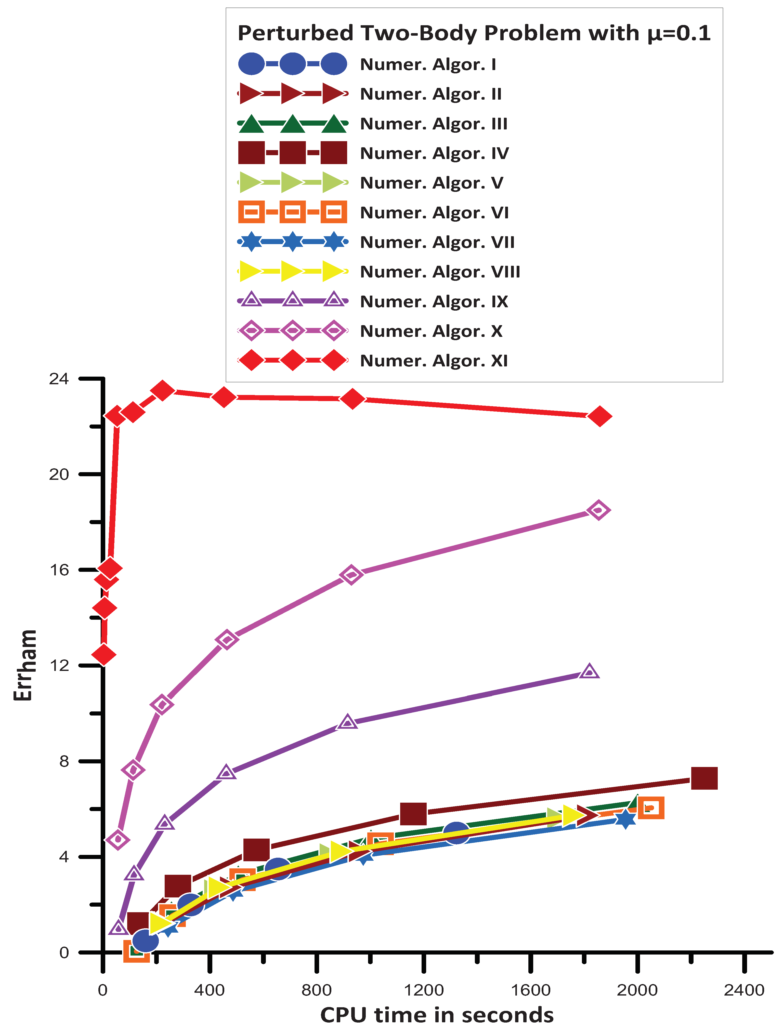
16.7. Perturbed Two-Body Gravitational Problem

16.7.1. Case $\mu =0.1$

Here, we take into account the perturbed two-body Kepler’s plane problem.

$$\begin{array}{c}\hfill s_1^{″}\left(x\right)=-\frac{s_1\left(x\right)}{{\left(s_1{\left(x\right)}^2+s_2{\left(x\right)}^2\right)}^{\frac{3}{2}}}-\mu (\mu +2)\frac{s_1\left(x\right)}{{\left(s_1{\left(x\right)}^2+s_2{\left(x\right)}^2\right)}^{\frac{5}{2}}},\\ \hfill s_1\left(0\right)=1,s_1^{\prime }\left(0\right)=0,\\ \hfill s_2^{″}\left(x\right)=-\frac{s_2\left(x\right)}{{\left(s_1{\left(x\right)}^2+s_2{\left(x\right)}^2\right)}^{\frac{3}{2}}}-\mu (\mu +2)\frac{s_2\left(x\right)}{{\left(s_1{\left(x\right)}^2+s_2{\left(x\right)}^2\right)}^{\frac{5}{2}}},\\ \hfill s_2\left(0\right)=0,s_2^{\prime }\left(0\right)=1+\mu .\end{array}$$

(107)

The exact solution is

$$\begin{array}{c}\hfill s_1\left(x\right)=cos(x+\mu x),\\ \hfill s_2\left(x\right)=sin(x+\mu x).\end{array}$$

(108)

For this problem, we use $\omega =\frac{\sqrt{1+\mu \left(\mu +2\right)}}{{\left(s_1{\left(x\right)}^2+s_2{\left(x\right)}^2\right)}^{\frac{3}{4}}}$.

Numerical solutions have been found for $0\le x\le$ 100,000 using $\mu =0.1$ and the techniques described in Section 16.1 for the system of Equation (107).

The following may be seen in Figure 18:

• Numer. Algor. I is more efficient than Numer. Algor. VII;
• Numer. Algor. I, Numer. Algor. II, Numer. Algor. V, Numer. Algor. VI, and Numer. Algor. VIII, have approximately the same efficiency;
• Numer. Algor. III is more efficient than Numer. Algor. I;
• Numer. Algor. IV is more efficient than Numer. Algor. III;
• Numer. Algor. IX is more efficient than Numer. Algor. IV;
• Numer. Algor. X is more efficient than Numer. Algor. IX;
• Numer. Algor. XI gives the most efficient results.

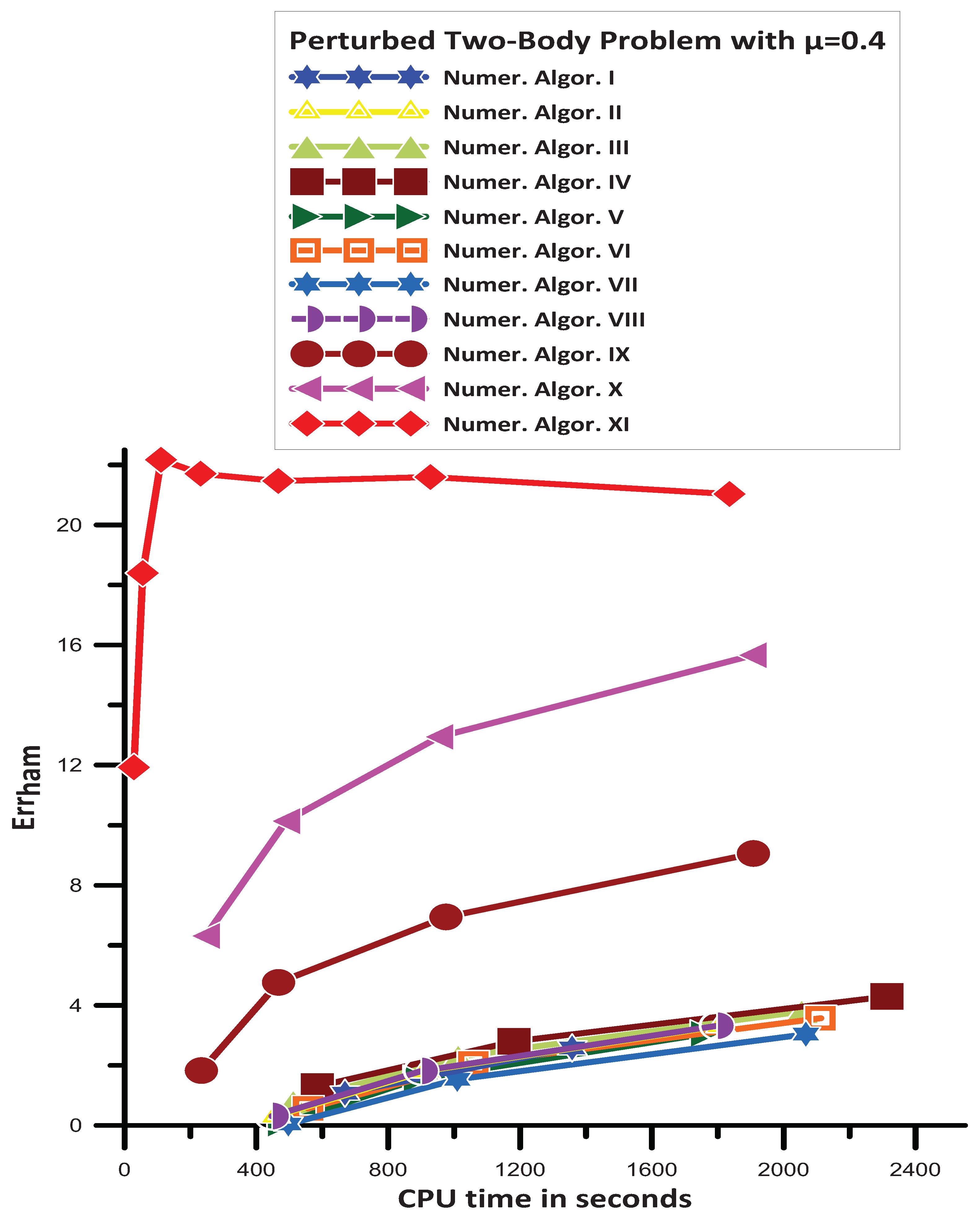
16.7.2. Case $\mu =0.4$

Numerical solutions have been found for $0\le x\le$ 100,000 using $\mu =0.1$ and the techniques described in Section 16.1 for the system of Equation (107).

The following may be seen in Figure 19:

• Numer. Algor. I is more efficient than Numer. Algor. VII;
• Numer. Algor. I, Numer. Algor. II, Numer. Algor. V, Numer. Algor. VI, and Numer. Algor. VIII, have approximately the same efficiency;
• Numer. Algor. III is more efficient than Numer. Algor. I;
• Numer. Algor. IV is more efficient than Numer. Algor. III;
• Numer. Algor. IX is more efficient than Numer. Algor. IV;
• Numer. Algor. X is more efficient than Numer. Algor. IX;
• Numer. Algor. XI gives the most efficient results.

Based on the numerical examples provided above, we may deduce:

• Results for all problems are most efficiently produced by the phase-fitted and amplification-fitted approach (Numer. Algor. XI);
• Results for the majority of problems are second-best when using the amplification-fitted Adams–Bashforth–Moulton Algorithm of second algebraic order with a phase-lag of order eight (Numer. Algor. X);
• Results for the majority of problems are third-best when using the amplification-fitted Adams–Bashforth–Moulton Algorithm of second algebraic order with a phase-lag of order six (Numer. Algor. IX).

In light of the above, it is clear that the strategies offered in this work that provide the best results are:

• The strategy that disregards the algebraic order of the procedure in favor of minimizing the phase-lag;
• Strategies that concentrate on eliminating phase-lag and the amplification factor

The effectiveness of frequency-dependent approaches, such as the recently presented ones, is clearly influenced by the parameter v that is chosen. This option may often be defined directly from the problem’s model in many cases. The literature (e.g., [123,124]) has proposed approaches for determining the parameter v in circumstances when this is not simple.

Remark 2.

One thing to keep in mind when solving systems of high-order ordinary differential equations using the recently introduced techniques is that there are already established ways to simplify such systems into first-order differential equations. For examples of such methods, see [125].

In order to solve systems of partial differential equations using the recently introduced techniques mentioned earlier, it is important to note that there are already established methods, see [126], that can reduce such a system to a system of first-order differential equations.

17. Conclusions

For implicit multistep approaches to first-order initial-value problems, we presented here the theory of phase-lag and amplification-error analysis. Several strategies for the construction of efficient predictor–corrector methods were offered, based on the theory described above and that developed in [115] for explicit methods. Our development efforts focused on the following strategies:

• Strategies for reducing the phase-lag;
• A strategy for the construction of an amplification-fitted method;
• A strategy for the construction of a phase–fitted method.

We created a number of multistep predictor–corrector approaches by using the aforementioned strategies. We based on the fourth algebraic order the Adams–Bashforth explicit method and on the fifth algebraic order Adams–Moulton implicit method.

The effectiveness of the aforementioned strategies was evaluated by applying them to many problems involving oscillating solutions.

It is worth mentioning that the idea put forward in this work and [115] is novel in the literature in relation to the development of:

• multistep methods for first-order initial-value problems with minimal phase-lag;
• phase-fitted and amplification-fitted multistep methods for first-order initial-value problems.

The same theory can be applied to all categories of multistep methods for first-order initial-value problem with oscillating solutions.

We also note that the methods presented in this paper can be applied to any problem with oscillating solution.

The computations were carried out using a 64-bit quadruple-precision arithmetic data type-compatible personal computer that conformed to the IEEE Standard 754, using a $FORTRAN$ package.

References

- Landau, L.D.; Lifshitz, F.M. Quantum Mechanics; Pergamon: New York, NY, USA, 1965. [Google Scholar]
- Prigogine, I.; Rice, S. (Eds.) Advances in Chemical Physics Vol. 93: New Methods in Computational Quantum Mechanics; John Wiley & Sons: Hoboken, NJ, USA, 1997. [Google Scholar]
- Simos, T.E. Numerical Solution of Ordinary Differential Equations with Periodical Solution. Ph.D. Thesis, National Technical University of Athens, Athens, Greece, 1990. (In Greek). [Google Scholar]
- Raptis, A.D. Exponential multistep methods for ordinary differential equations. Bull. Greek Math. Soc. 1984, 25, 113–126. [Google Scholar]
- Vigo-Aguiar, J.; Ferrandiz, J.M. A general procedure for the adaptation of multistep algorithms to the integration of oscillatory problems. SIAM J. Numer. Anal. 1998, 35, 1684–1708. [Google Scholar] [CrossRef]
- Vigo-Aguiar, J. Mathematical Methods for the Numerical Propagation of Satellite Orbits. Ph.D. Thesis, University of Valladolid, Valladolid, Spain, 1993. (In Spanish). [Google Scholar]
- Ixaru, L.G. Numerical Methods for Differential Equations and Applications; Reidel: Dordrecht, The Netherlands; Boston, MA, USA; Lancaster, UK, 1984. [Google Scholar]
- Quinlan, G.D.; Tremaine, S. Symmetric multistep methods for the numerical integration of planetary orbits. Astron. J. 1990, 100, 1694–1700. [Google Scholar] [CrossRef]
- Lyche, T. Chebyshevian multistep methods for ordinary differential equations. Numer. Math. 1972, 10, 65–75. [Google Scholar] [CrossRef]
- Raptis, A.D.; Allison, A.C. Exponential-fitting methods for the numerical solution of the Schrödinger equation. Comput. Phys. Commun. 1978, 14, 1–5. [Google Scholar] [CrossRef]
- Konguetsof, A.; Simos, T.E. On the construction of Exponentially-Fitted Methods for the Numerical Solution of the Schrödinger Equation. J. Comput. Math. Sci. Eng. 2001, 1, 143–165. [Google Scholar] [CrossRef]
- Simos, T.E. Atomic Structure Computations in Chemical Modelling: Applications and Theory; Hinchliffe, A., Ed.; The Royal Society of Chemistry: London, UK, 2000; pp. 38–142. [Google Scholar]
- Simos, T.E.; Vigo-Aguiar, J. On the construction of efficient methods for second order IVPs with oscillating solution. Int. J. Mod. Phys. C 2001, 10, 1453–1476. [Google Scholar] [CrossRef]
- Dormand, J.R.; El-Mikkawy, M.E.A.; Prince, P.J. Families of Runge–Kutta-Nyström formulae. IMA J. Numer. Anal. 1987, 7, 235–250. [Google Scholar] [CrossRef]
- Van De Vyver, H. A Symplectic Exponentially Fitted Modified Runge–Kutta-Nyström Method for the Numerical Integration of Orbital Problems. New Astron. 2005, 10, 261–269. [Google Scholar] [CrossRef]
- Van De Vyver, H. On the Generation of P-Stable Exponentially Fitted Runge–Kutta-Nyström Methods By Exponentially Fitted Runge–Kutta Methods. J. Comput. Appl. Math. 2006, 188, 309–318. [Google Scholar] [CrossRef]
- Franco, J.M.; Khiar, Y.; Rández, L. Two new embedded pairs of explicit Runge–Kutta Methods adapted to the numerical solution of oscillatory problems. Appl. Math. Comput. 2015, 252, 45–57. [Google Scholar] [CrossRef]
- Franco, J.M.; Gomez, I. Symplectic explicit Methods of Runge–Kutta-Nyström type for solving perturbed oscillators. J. Comput. Appl. Math. 2014, 260, 482–493. [Google Scholar] [CrossRef]
- Franco, J.M.; Gomez, I. Some procedures for the construction of high-order exponentially fitted Runge–Kutta-Nyström Methods of explicit type. Comput. Phys. Commun. 2013, 184, 1310–1321. [Google Scholar] [CrossRef]
- Calvo, M.; Franco, J.M.; Montijano, J.I.; Rández, L. On some new low storage implementations of time advancing Runge–Kutta Methods. J. Comput. Appl. Math. 2012, 236, 3665–3675. [Google Scholar] [CrossRef]
- Calvo, M.; Franco, J.M.; Montijano, J.I.; Rández, L. Symmetric and symplectic exponentially fitted Runge–Kutta Methods of high order. Comput. Phys. Commun. 2010, 181, 2044–2056. [Google Scholar] [CrossRef]
- Calvo, M.; Franco, J.M.; Montijano, J.I.; Rández, L. On high order symmetric and symplectic trigonometrically fitted Runge–Kutta Methods with an even number of stages. BIT Numer. Math. 2010, 50, 3–21. [Google Scholar] [CrossRef]
- Franco, J.M.; Gomez, I. Accuracy and linear Stability of RKN Methods for solving second-order stiff problems. Appl. Numer. Math. 2009, 59, 959–975. [Google Scholar] [CrossRef]
- Calvo, M.; Franco, J.M.; Montijano, J.I.; Rández, L. Sixth-order symmetric and symplectic exponentially fitted Runge–Kutta Methods of the Gauss type. J. Comput. Appl. Math. 2009, 22, 387–398. [Google Scholar] [CrossRef]
- Calvo, M.; Franco, J.M.; Montijano, J.I.; Rández, L. Structure preservation of exponentially fitted Runge–Kutta Methods. J. Comput. Appl. Math. 2008, 218, 421–434. [Google Scholar] [CrossRef]
- Calvo, M.; Franco, J.M.; Montijano, J.I.; Rández, L. Sixth-order symmetric and symplectic exponentially fitted modified Runge–Kutta Methods of Gauss type. Comput. Phys. Commun. 2008, 178, 732–744. [Google Scholar] [CrossRef]
- Franco, J.M. Exponentially fitted symplectic integrators of RKN type for solving oscillatory problems. Comput. Phys. Commun. 2007, 177, 479–492. [Google Scholar] [CrossRef]
- Franco, J.M. New Methods for oscillatory systems based on ARKN Methods. Appl. Numer. Math. 2006, 56, 1040–1105. [Google Scholar] [CrossRef]
- Franco, J.M. Runge–Kutta-Nyström Methods adapted to the numerical integration of perturbed oscillators. Comput. Phys. Commun. 2002, 147, 770–787. [Google Scholar] [CrossRef]
- Franco, J.M. Stability of explicit ARKN Methods for perturbed oscillators. J. Comput. Appl. Math. 2005, 173, 389–396. [Google Scholar] [CrossRef]
- Wu, X.Y.; You, X.; Li, J.Y. Note on derivation of order conditions for ARKN Methods for perturbed oscillators. Comput. Phys. Commun. 2009, 180, 1545–1549. [Google Scholar] [CrossRef]
- Tocino, A.; Vigo-Aguiar, J. Symplectic conditions for exponential fitting Runge–Kutta-Nyström Methods. Math. Comput. Modell. 2005, 42, 873–876. [Google Scholar] [CrossRef]
- Van de Vyver, H. Comparison of some special optimized fourth-order Runge–Kutta Methods for the numerical solution of the Schrödinger equation. Comput. Phys. Commun. 2005, 166, 109–122. [Google Scholar] [CrossRef]
- Van de Vyver, H. Frequency evaluation for exponentially fitted Runge–Kutta Methods. J. Comput. Appl. Math. 2005, 184, 442–463. [Google Scholar] [CrossRef]
- Vigo-Aguiar, J.; Martín-Vaquero, J.; Ramos, H. Exponential fitting BDF-Runge–Kutta Algorithms. Comput. Phys. Commun. 2008, 178, 15–34. [Google Scholar] [CrossRef]
- Demba, M.A.; Senu, N.; Ramos, H.; Kumam, P.; Watthayu, W. A Phase– and Amplification–Fitted 5(4) Diagonally Implicit Runge–Kutta–Nyström Pair for Oscillatory Systems. Bull. Iran. Math. Soc. 2023, 49, 24. [Google Scholar] [CrossRef]
- Demba, M.A.; Ramos, H.; Watthayu, W.; Ahmed, I. A New Phase- and Amplification-Fitted Sixth-Order Explicit RKN Method to Solve Oscillating Systems. Thai J. Math. 2023, 21, 219–236. [Google Scholar]
- Monovasilis, T.; Kalogiratou, Z. High Order Two-Derivative Runge–Kutta Methods with Optimized Dispersion and Dissipation Error. Mathematics 2021, 9, 232. [Google Scholar] [CrossRef]
- Ahmad, N.A.; Senu, N.; Ibrahim, Z.B.; Othman, M.; Ismail, Z. Higher Order Three Derivative Runge–Kutta Method with Phase–Fitting and Amplification–Fitting Technique for Periodic IVPs. Malaysian J. Math. Sci. 2020, 14, 403–418. [Google Scholar]
- Lee, K.; Alias, M.A.; Senu, N.; Ahmadian, A. On efficient frequency-dependent parameters of explicit two-derivative improved Runge–Kutta-Nyström method with application to two-body problem. Alex. Eng. J. 2023, 72, 605–620. [Google Scholar] [CrossRef]
- Chien, L.K.; Senu, N.; Ahmadian, A.; Ibrahim, S.N.I. Efficient Frequency-Dependent Coefficients of Explicit Improved Two-Derivative Runge–Kutta Type Methods for Solving Third- Order IVPs. Pertanika J. Sci. Technol. 2023, 31, 843–873. [Google Scholar] [CrossRef]
- Demba, M.A.; Ramos, H.; Kumam, P.; Watthayu, W.; Senu, N.; Ahmed, I. A trigonometrically adapted 6(4) explicit Runge–Kutta-Nyström pair to solve oscillating systems. Math. Methods Appl. Sci. 2023, 46, 560–578. [Google Scholar] [CrossRef]
- Chen, B.Z.; Zhai, W.J. Optimal three-stage implicit exponentially-fitted RKN methods for solving second-order ODEs. Calcolo 2022, 59, 14. [Google Scholar] [CrossRef]
- Senu, N.; Ahmad, N.A.; Othman, M.; Ibrahim, Z.B. Numerical study for periodical delay differential equations using Runge–Kutta with trigonometric interpolation. Comput. Appl. Math. 2022, 41, 25. [Google Scholar] [CrossRef]
- Zhai, W.J.; Fu, S.H.; Zhou, T.C.; Xiu, C. Exponentially-fitted and trigonometrically-fitted implicit RKN methods for solving y′′=f(t,y). J. Appl. Math. Comput. 2022, 68, 1449–1466. [Google Scholar] [CrossRef]
- Senu, N.; Lee, K.C.; Ismail, W.F.W.; Ahmadian, A.; Ibrahim, S.N.I.; Laham, M. Improved Runge–Kutta Method with Trigonometrically-Fitting Technique for Solving Oscillatory Problem. Malaysian J. Math. Sci. 2021, 15, 253–266. [Google Scholar]
- Fang, Y.L.; Yang, Y.P.; You, X. An explicit trigonometrically fitted Runge–Kutta method for stiff and oscillatory problems with two frequencies. Int. J. Comput. Math. 2020, 97, 85–94. [Google Scholar] [CrossRef]
- Dormand, J.R.; Prince, P.J. A family of embedded Runge–Kutta formulae. J. Comput. Appl. Math. 1980, 6, 19–26. [Google Scholar] [CrossRef]
- Kalogiratou, Z.; Monovasilis, T.; Psihoyios, G.; Simos, T.E. Runge–Kutta type methods with special properties for the numerical integration of ordinary differential equations. Phys. Rep. 2014, 536, 75–146. [Google Scholar] [CrossRef]
- Shokri, A.; Khalsaraei, M.M. A new family of explicit linear two-step singularly P-stable Obrechkoff methods for the numerical solution of second-order IVPs. Appl. Math. Comput. 2020, 376, 125116. [Google Scholar] [CrossRef]
- Abdulganiy, R.I.; Ramos, H.; Okunuga, S.A.; Majid, Z.A. A trigonometrically fitted intra-step block Falkner method for the direct integration of second-order delay differential equations with oscillatory solutions. Afr. Mat. 2023, 34, 36. [Google Scholar] [CrossRef]
- Salih, M.M.; Ismail, F. Trigonometrically-Fitted Fifth Order Four-Step Predictor-Corrector Method for Solving Linear Ordinary Differential Equations with Oscillatory Solutions. Malaysian J. Math. Sci. 2022, 16, 739–748. [Google Scholar] [CrossRef]
- Godwin, O.J.; Adewale, O.S.; Otuwatomi, O.P. An efficient block solver of trigonometrically fitted method for stiff odes. Adv. Differ. Equ. Control Process. 2022, 28, 73–98. [Google Scholar] [CrossRef]
- Lee, K.C.; Senu, N.; Ahmadian, A.; Ibrahim, S.N.I. High-order exponentially fitted and trigonometrically fitted explicit two-derivative Runge–Kutta-type methods for solving third-order oscillatory problems. Math. Sci. 2022, 16, 281–297. [Google Scholar] [CrossRef]
- Obaidat, S.; Butt, R. A new implicit symmetric method of sixth algebraic order with vanished phase-lag and its first derivative for solving Schrodinger’s equation. Open Math. 2021, 19, 225–237. [Google Scholar] [CrossRef]
- Shokri, A.; Neta, B.; Khalsaraei, M.M.; Rashidi, M.M.; Mohammad-Sedighi, H. A Singularly P-Stable Multi-Derivative Predictor Method for the Numerical Solution of Second-Order Ordinary Differential Equations. Mathematics 2021, 9, 806. [Google Scholar] [CrossRef]
- Fang, Y.L.; Huang, T.; You, X.; Zheng, J.; Wang, B. Two-frequency trigonometrically-fitted and symmetric linear multi-step methods for second-order oscillators. J. Comput. Appl. Math. 2021, 392, 113312. [Google Scholar] [CrossRef]
- Chun, C.; Neta, B. Trigonometrically-Fitted Methods: A Review. Mathematics 2019, 7, 1197. [Google Scholar] [CrossRef]
- Anastassi, Z.A.; Simos, T.E. Numerical multistep methods for the efficient solution of quantum mechanics and related problems. Phys. Rep. 2009, 482–483, 1–240. [Google Scholar] [CrossRef]
- Chawla, M.M.; Rao, P.S. A Noumerov-Type Method with Minimal Phase–Lag for the Integration of 2nd Order Periodic Initial-Value Problems. J. Comput. Appl. Math. 1984, 11, 277–281. [Google Scholar] [CrossRef]
- Thomas, R.M. Phase properties of high order almost P-stable formulae. BIT 1984, 24, 225–238. [Google Scholar]
- Chawla, M.M.; Rao, P.S.; Neta, B. 2-Step 4Th-Order P-Stable Methods with Phase–Lag of Order 6 for Y″ = F(T,Y). J. Comput. Appl. Math. 1986, 16, 233–236. [Google Scholar] [CrossRef]
- Chawla, M.M.; Rao, P.S. An Explicit 6Th-Order Method with Phase–Lag of Order 8 for Y″ = F(T, Y). J. Comput. Appl. Math. 1987, 17, 365–368. [Google Scholar]
- JColeman, J.P. Numerical-Methods for Y″ = F(X,Y) Via Rational-Approximations for the Cosine. IMA J. Numer. Anal. 1989, 9, 145–165. [Google Scholar]
- Coleman, J.P.; Ixaru, L.G. P-Stability and Exponential-Fitting Methods for Y″ = F(X, Y). IMA J. Numer. Anal. 1996, 16, 179–199. [Google Scholar] [CrossRef]
- Coleman, J.P.; Duxbury, S.C. Mixed Collocation Methods for Y” = F(X,Y). J. Comput. Appl. Math. 2000, 126, 47–75. [Google Scholar] [CrossRef]
- Ixaru, L.G.; Berceanu, S. Coleman Method Maximally Adapted to the Schrödinger-Equation. Comput. Phys. Commun. 1987, 44, 11–20. [Google Scholar] [CrossRef]
- Ixaru, L.G.; Rizea, M. Numerov Method Maximally Adapted to the Schrödinger-Equation. J. Comput. Phys. 1987, 73, 306–324. [Google Scholar] [CrossRef]
- Ixaru, L.G.; Vanden Berghe, G.; De Meyer, H.; Van Daele, M. Four-Step Exponential-Fitted Methods for Nonlinear Physical Problems. Comput. Phys. Commun. 1997, 100, 56–70. [Google Scholar] [CrossRef]
- Ixaru, L.G.; Rizea, M. Four Step Methods for Y″ = F(X,Y). J. Comput. Appl. Math. 1997, 79, 87–99. [Google Scholar] [CrossRef]
- Van Daele, M.; Vanden Berghe, G.; De Meyer, H.; Ixaru, L.G. Exponential-Fitted Four-Step Methods for Y” = F(X,Y). Int. J. Comput. Math. 1998, 66, 299–309. [Google Scholar] [CrossRef]
- Ixaru, L.G.; Paternoster, B. A Conditionally P-Stable Fourth-Order Exponential-Fitting Method for Y” = F(X, Y). J. Comput. Appl. Math. 1999, 106, 87–98. [Google Scholar] [CrossRef]
- Ixaru, L.G. Numerical operations on oscillatory functions. Comput. Chem. 2001, 25, 39–53. [Google Scholar] [CrossRef] [PubMed]
- Ixaru, L.G.; Vanden Berghe, G.; De Meyer, H. Exponentially Fitted Variable Two-Step BDF Algorithm for First Order Odes. Comput. Phys. Commun. 2003, 150, 116–128. [Google Scholar] [CrossRef]
- Ixaru, L.G.; Rizea, M. Comparison of some four-Step Methods for the numerical solution of the Schrödinger equation. Comput. Phys. Commun. 1985, 38, 329–337. [Google Scholar] [CrossRef]
- Ixaru, L.G.; Rizea, M. A Numerov-like scheme for the numerical solution of the Schrödinger equation in the deep continuum spectrum of energies. Comput. Phys. Commun. 1980, 19, 23–27. [Google Scholar] [CrossRef]
- Avdelas, G.; Simos, T.E. A generator of high-order embedded P-stable method for the numerical solution of the Schrödinger equation. J. Comput. Appl. Math. 1996, 72, 345–358. [Google Scholar] [CrossRef]
- Chawla, M.M.; Rao, P.S. An Noumerov-type Method with minimal phase-lag for the integration of second order periodic initial-value problems II Explicit Method. J. Comput. Appl. Math. 1986, 15, 329–337. [Google Scholar] [CrossRef]
- Franco, J.M. Runge–Kutta methods adapted to the numerical integration of oscillatory problems. Appl. Numer. Math. 2004, 50, 427–443. [Google Scholar] [CrossRef]
- Rizea, M. Exponential fitting Method for the time-dependent Schrödinger equation. J. Math. Chem. 2010, 48, 55–65. [Google Scholar] [CrossRef]
- Ixaru, L.G.; Rizea, M.; Vanden Berghe, G.; De Meyer, H. Weights of the Exponential Fitting Multistep Algorithms for First-Order Odes. J. Comput. Appl. Math. 2001, 132, 83–93. [Google Scholar] [CrossRef]
- Raptis, A.D.; Cash, J.R. Exponential and Bessel Fitting Methods for the Numerical-Solution of the Schrödinger-Equation. Comput. Phys. Commun. 1987, 44, 95–103. [Google Scholar] [CrossRef]
- Simos, T.E. Predictor-corrector phase-fitted methods for y”=f(x,y) and an application to the Schrödinger equation. Int. J. Quantum Chem. 1995, 53, 473–483. [Google Scholar] [CrossRef]
- Raptis, A.D. Exponentially-Fitted Solutions of the Eigenvalue Shrödinger Equation with Automatic Error Control. Comput. Phys. Commun. 1983, 28, 427–431. [Google Scholar] [CrossRef]
- Raptis, A.D. 2-Step Methods for the Numerical-Solution of the Schrödinger-Equation. Comput. Phys. Commun. 1982, 28, 373–378. [Google Scholar] [CrossRef]
- Raptis, A.D. On the Numerical-Solution of the Schrödinger-Equation. Comput. Phys. Commun. 1981, 24, 1–4. [Google Scholar] [CrossRef]
- Raptis, A.D. Exponential-Fitting Methods for the Numerical-Integration of the 4Th-Order Differential-Equation Yiv + F.Y = G. Computing 1980, 24, 241–250. [Google Scholar] [CrossRef]
- Van Daele, M.; Vanden Berghe, G. P-stable exponentially-fitted Obrechkoff Methods of arbitrary order for second-order differential equations. Numer. Algorithms 2007, 46, 333–350. [Google Scholar] [CrossRef]
- Fang, Y.; Wu, X. A Trigonometrically Fitted Explicit Numerov-Type Method for Second-Order Initial Value Problems with Oscillating Solutions. Appl. Numer. Math. 2008, 58, 341–351. [Google Scholar] [CrossRef]
- Vanden Berghe, G.; Van Daele, M. Exponentially-fitted Obrechkoff Methods for second-order differential equations. Appl. Numer. Math. 2009, 59, 815–829. [Google Scholar] [CrossRef]
- Hollevoet, D.; Van Daele, M.; Vanden Berghe, G. the Optimal Exponentially-Fitted Numerov Method for Solving Two-Point Boundary Value Problems. J. Comput. Appl. Math. 2009, 230, 260–269. [Google Scholar] [CrossRef]
- Franco, J.M.; Rández, L. Explicit exponentially fitted two-Step hybrid Methods of high order for second-order oscillatory IVPs. Appl. Math. Comput. 2016, 273, 493–505. [Google Scholar] [CrossRef]
- Franco, J.M.; Gomez, I.; Rández, L. Optimization of explicit two-Step hybrid Methods for solving orbital and oscillatory problems. Comput. Phys. Commun. 2014, 185, 2527–2537. [Google Scholar] [CrossRef]
- Franco, J.M.; Gomez, I. Trigonometrically fitted nonlinear two-Step Methods for solving second order oscillatory IVPs. Appl. Math. Comput. 2014, 232, 643–657. [Google Scholar] [CrossRef]
- Konguetsof, A. A generator of families of two-Step numerical Methods with free parameters and minimal phase-lag. J. Math. Chem. 2017, 55, 1808–1832. [Google Scholar] [CrossRef]
- Konguetsof, A. A hybrid Method with phase-lag and derivatives equal to zero for the numerical integration of the Schrödinger equation. J. Math. Chem. 2011, 49, 1330–1356. [Google Scholar] [CrossRef]
- Van de Vyver, H. A phase-fitted and amplification-fitted explicit two-Step hybrid Method for second-order periodic initial value problems. Int. J. Mod. Phys. C 2006, 17, 663–675. [Google Scholar] [CrossRef]
- Van de Vyver, H. An explicit Numerov-type Method for second-order differential equations with oscillating solutions. Comput. Math. Appl. 2007, 53, 1339–1348. [Google Scholar] [CrossRef]
- Fang, Y.; Wu, X. A trigonometrically fitted explicit hybrid Method for the numerical integration of orbital problems. Appl. Math. Comput. 2007, 189, 178–185. [Google Scholar] [CrossRef]
- Van de Vyver, H. Phase-fitted and amplification-fitted two-Step hybrid Methods for y” = f (x, y). J. Comput. Appl. Math. 2007, 209, 33–53. [Google Scholar] [CrossRef]
- Van de Vyver, H. Efficient one-Step Methods for the Schrödinger equation. MATCH-Commun. Math. Comput. Chem. 2008, 60, 711–732. [Google Scholar]
- Martín-Vaquero, J.; Vigo-Aguiar, J. Exponential fitted Gauss, Radau and Lobatto Methods of low order. Numer. Algorithms 2008, 48, 327–346. [Google Scholar]
- Konguetsof, A. A new two-Step hybrid Method for the numerical solution of the Schrödinger equation. J. Math. Chem. 2010, 47, 871–890. [Google Scholar] [CrossRef]
- Hendi, F.A. P-Stable Higher Derivative Methods with Minimal Phase–Lag for Solving Second Order Differential Equations. J. Appl. Math. 2011, 2011, 407151. [Google Scholar] [CrossRef]
- Wang, Z.; Zhao, D.; Dai, Y.; Wu, D. An improved trigonometrically fitted P-stable Obrechkoff Method for periodic initial-value problems. Proc. R. Soc. A-Math. Phys. Eng. Sci. 2005, 461, 1639–1658. [Google Scholar] [CrossRef]
- Van Daele, M.; Vanden Berghe, G.; De Meyer, H. Properties and Implementation of R-Adams Methods Based On Mixed-Type Interpolation. Comput. Phys. Commun. 1995, 30, 37–54. [Google Scholar] [CrossRef]
- Wang, Z. Trigonometrically-fitted Method with the Fourier frequency spectrum for undamped duffing equation. Comput. Phys. Commun. 2006, 174, 109–118. [Google Scholar] [CrossRef]
- Wang, Z. Trigonometrically-fitted Method for a periodic initial value problem with two frequencies. Comput. Phys. Commun. 2006, 175, 241–249. [Google Scholar] [CrossRef]
- Tang, C.; Yan, H.; Zhang, H.; Li, W. The various order explicit multistep exponential fitting for systems of ordinary differential equations. J. Comput. Appl. Math. 2004, 169, 171–182. [Google Scholar] [CrossRef]
- Tang, C.; Yan, H.; Zhang, H.; Chen, Z.; Liu, M.; Zhang, G. The arbitrary order implicit multistep schemes of exponential fitting and their applications. J. Comput. Appl. Math. 2005, 173, 155–168. [Google Scholar] [CrossRef]
- Coleman, J.P.; Ixaru, L.G. Truncation Errors in exponential fitting for oscillatory problems. SIAM J. Numer. Anal. 2006, 44, 1441–1465. [Google Scholar] [CrossRef]
- Paternoster, B. Present state-of-the-art in exponential fitting. A contribution dedicated to Liviu Ixaru on their 70th birthday. Comput. Phys. Commun. 2012, 183, 2499–2512. [Google Scholar] [CrossRef]
- Wang, Z. Obrechkoff one-Step Method fitted with Fourier spectrum for undamped Duffing equation. Comput. Phys. Commun. 2006, 175, 692–699. [Google Scholar] [CrossRef]
- Wang, C.; Wang, Z. A P-stable eighteenth-order six-Step Method for periodic initial value problems. Int. J. Mod. Phys. C 2007, 18, 419–431. [Google Scholar] [CrossRef]
- Simos, T.E. A New Methodology for the Development of Efficient Multistep Methods for First–Order IVPs with Oscillating Solutions. Mathematics 2024, 12, 504. [Google Scholar] [CrossRef]
- Stiefel, E.; Bettis, D.G. Stabilization of Cowell’s method. Numer. Math. 1969, 13, 154–175. [Google Scholar] [CrossRef]
- Fehlberg, E. Classical fifth-, Sixth-, Seventh-, and Eighth-Order Runge–Kutta Formulas with Stepsize Control. NASA Technical Report 287. 1968. Available online: https://ntrs.nasa.gov/api/citations/19680027281/downloads/19680027281.pdf (accessed on 30 March 2024).
- Cash, J.R.; Karp, A.H. A variable order Runge–Kutta method for initial value problems with rapidly varying right-hand sides. ACM Trans. Math. Softw. 1990, 16, 201–222. [Google Scholar] [CrossRef]
- Franco, J.; Gómez, I.; Rández, L. Four-stage symplectic and P–stable SDIRKN methods with dispersion of high order. Numer. Algorithms 2001, 26, 347–363. [Google Scholar] [CrossRef]
- Franco, J.M.; Palacios, M. High-order P-stable multistep methods. J. Comput. Appl. Math. 1990, 30, 1–10. [Google Scholar] [CrossRef]
- Simos, T.E. New Open Modified Newton Cotes Type Formulae as Multilayer Symplectic Integrators. Appl. Math. Modell. 2013, 37, 1983–1991. [Google Scholar] [CrossRef]
- Petzold, L.R. An efficient numerical method for highly oscillatory ordinary differential equations. SIAM J. Numer. Anal. 1981, 18, 455–479. [Google Scholar] [CrossRef]
- Ramos, H.; Vigo-Aguiar, J. On the frequency choice in trigonometrically fitted methods. Appl. Math. Lett. 2010, 11, 1378–1381. [Google Scholar] [CrossRef]
- Ixaru, L.G.; Vanden Berghe, G.; De Meyer, H. Frequency evaluation in exponential fitting multistep algorithms for ODEs. J. Comput. Appl. Math. 2002, 140, 423–434. [Google Scholar] [CrossRef]
- Boyce, W.E.; DiPrima, R.C.; Meade, D.B. Elementary Differential Equations and Boundary Value Problems, 11th ed.; John Wiley & Sons: Hoboken, NJ, USA, 2017. [Google Scholar]
- Lawrence, C. Evans, Partial Differential Equations, 2nd ed.; American Mathematical Society: Providence, RI, USA, 2010; Chapter 3; p. 91135. [Google Scholar]
Figure 1.
Stability Region for the classical Fourth-Order Adams–Bashforth Method (Algorithm I). The axes of the stability region are H and .
Figure 2.
Stability Region of the Amplification-Fitted Adams–Bashforth Method of Algebraic Order Four with Phase-Lag of Order Four (Algorithm II). The axes of the stability region are H and .
Figure 3.
Stability Region of the Amplification-Fitted Adams–Bashforth Method of Algebraic Order Three with Phase-Lag of Order Six (Algorithm III). The axes of the stability region are H and .
Figure 4.
Stability Region of the Amplification-Fitted Adams–Bashforth Method of Algebraic Order Four (Algorithm IV). The axes of the stability region are H and .
Figure 5.
Stability Region of the Phase-Fitted and Amplification-Fitted Adams–Bashforth Method of Algebraic Order Four (Algorithm V). The axes of the stability region are H and .
Figure 6.
Stability Region of Adams–Moulton Fifth Algebraic Order Method (Algorithm VI). The axes of the stability region are H and .
Figure 7.
Stability Region of the Amplification-Fitted Adams–Moulton Method of Algebraic Order Five with Phase-Lag of Order Four (Algorithm VII). The axes of the stability region are H and .
Figure 8.
Stability Region of the Amplification-Fitted Adams–Moulton Method of Algebraic Order Two with Phase-Lag of Order Six (Algorithm VIII). The axes of the stability region are H and .
Figure 9.
Stability Region of the Amplification-Fitted Adams–Moulton Method of Algebraic Order Two with Phase-Lag of Order Eight (Algorithm IX). The axes of the stability region are H and .
Figure 10.
Stability Region of the Amplification-Fitted Adams–Moulton Method of Algebraic Order Five (Algorithm X). The axes of the stability region are H and .
Figure 11.
Stability Region of the Phase-Fitted and Amplification-Fitted Adams–Moulton Method of Algebraic Order Five (Algorithm XI). The axes of the stability region are H and .
Figure 12.
Numerical results for the problem of Stiefel and Bettis [116].
Figure 13.
Numerical results for the problem of Franco et al. [119].
Figure 14.
Numerical results for the problem of Franco and Palacios [120].
Figure 15.
Numerical results for the Nonlinear Orbital problem of [121].
Figure 16.
Numerical results for the nonlinear problem of [122].
Figure 17.
Numerical results for two-body gravitational problem (Kepler’s plane problem).
Figure 18.
Numerical results for perturbed two-body gravitational problem (perturbed Kepler’s problem) with .
Figure 19.
Disclaimer/Publisher’s Note: The statements, opinions and data contained in all publications are solely those of the individual author(s) and contributor(s) and not of MDPI and/or the editor(s). MDPI and/or the editor(s) disclaim responsibility for any injury to people or property resulting from any ideas, methods, instructions or products referred to in the content. |
© 2024 by the author. Licensee MDPI, Basel, Switzerland. This article is an open access article distributed under the terms and conditions of the Creative Commons Attribution (CC BY) license (https://creativecommons.org/licenses/by/4.0/).
Share and Cite
MDPI and ACS Style
Simos, T.E. Efficient Multistep Algorithms for First-Order IVPs with Oscillating Solutions: II Implicit and Predictor–Corrector Algorithms. Symmetry 2024, 16, 508. https://doi.org/10.3390/sym16050508
AMA Style
Simos TE. Efficient Multistep Algorithms for First-Order IVPs with Oscillating Solutions: II Implicit and Predictor–Corrector Algorithms. Symmetry. 2024; 16(5):508. https://doi.org/10.3390/sym16050508
Chicago/Turabian StyleSimos, Theodore E. 2024. "Efficient Multistep Algorithms for First-Order IVPs with Oscillating Solutions: II Implicit and Predictor–Corrector Algorithms" Symmetry 16, no. 5: 508. https://doi.org/10.3390/sym16050508
Note that from the first issue of 2016, this journal uses article numbers instead of page numbers. See further details here.