
Construction of Ruled Surfaces from the W-Curves and Their Characterizations in


1
Department of Mathematics and Statistics, College of Science, King Faisal University, AL-Ahsa, Hafuf 31982, Saudi Arabia
2
Department of Mathematics, Faculty of Science, Assiut University, Assiut 71516, Egypt
3
Department of Mathematics, Faculty of Science, Sohag University, Sohag 82524, Egypt
4
Department of Mathematics, Applied College, Northern Border University, Rafha 91431, Saudi Arabia
*
Author to whom correspondence should be addressed.
Symmetry 2024, 16(5), 509; https://doi.org/10.3390/sym16050509
Submission received: 27 March 2024
/
Revised: 15 April 2024
/
Accepted: 17 April 2024
/
Published: 23 April 2024
(This article belongs to the Section Mathematics)
Abstract
:Ruled surfaces are considered one of the significant aspects of differential geometry. These surfaces are formed by the motion of a straight line called a generator, and every curve that intersects all the generators is called a directrix. In the present research paper, we explore a family of ruled surfaces constructed from circular helices (W-curve) using the Frenet frame in the Euclidean space . We derive the explicit formulas for the second mean curvature and second Gaussian curvature. We present some ruled surfaces, and we describe their properties. In addition, we determine the sufficient conditions for these surfaces to be minimal, flat, II-minimal, and II-flat. Also, we obtain sufficient conditions for the base curve for these ruled surfaces to be a geodesic curve, an asymptotic line, and a principal line. Furthermore, we present an application for a ruled surface whose base curve is a circular helix, we compute some quantities for this surface such as the mean curvature and Gaussian curvatures and we plot the ruled surface with its base curve, and at symmetric points and along a symmetry axis.
Keywords:
ruled surfaces; circular helix; W-curves; II-minimal surfaces; II-flat surfaces; second mean curvature; second Gaussian curvatureMSC:
53A04; 53A05; 53A10; 53C401. Introduction
The primary objective of classical differential geometry is to comprehend the characteristics of specific types of surfaces in , including developable surfaces, ruled surfaces, minimal surfaces, and other related surfaces. Ruled surfaces (R-S) in Euclidean 3-space are geometric entities formed by straight lines, called rulings, that move through space while remaining tangent to a fixed line, known as the directrix. These surfaces have practical applications in fields such as architecture and computer graphics. Understanding their characteristics contributes to a deeper comprehension of geometry and its real-world implications.
Many researchers studied the (R-S) and their diverse characteristics. Gürsoy [1] analyzed the dual integral invariant of a closed ruled surface and presented some new results of the geometric interpretations for the real angle of pitch and the real pitch of a closed ruled surface. Köse [2] expressed the pitch and the angle of pitch of a closed ruled surface in terms of the integral invariants for the dual spherical closed curve that corresponds to the closed ruled surface. Turgut, et al. [3,4] investigated the properties of timelike (R-S) in Minkowski 3-space, along with the structure of developable timelike (R-S). The curve of striction, the central point, and the distribution parameter of these surfaces were also discussed. The angles between normal vectors at various sites on a ruling, the behavior of tangent planes along a ruling, and the unique value of the distribution parameter along a ruling were covered.
Ali et al. [5,6,7] investigated the mathematical description of helical structures in Euclidean 3-space, specifically, general helices and their position vectors concerning the Frenet frame for both general helices and slant helices. In addition, examples such as circular general helices, spherical general helices, Salkowski curves, and circular slant helices were presented.
Barros [8] proposed Lancret’s theorem for general helices in a three-dimensional real-space form. This theorem distinguishes the relationship between hyperbolic and spherical geometries, furthermore studying the problems related to general helices in the 3-sphere, including the closed curve problem and solving natural equations.
Ilarslan, et al. [9] focused on studying the position vectors of timelike and null helices in Minkowski space . These curves have constant curvatures, and their position vectors are utilized to characterize timelike and null helices with images on the Lorentzian sphere or pseudo-hyperbolical space .
Monterde [10] described a family of curves with constant curvature and non-constant torsion. These curves are characterized as space curves, and their normal vectors form a constant angle with a fixed line. The relationship between these curves and rational curves using a double Pythagorean hodograph was explored. In addition, a method for constructing closed curves with constant curvature and continuous torsion using pieces of Salkowski curves was presented.
Classical differential geometry employs intrinsic equations to determine the position vectors of curves, such as and , where and represent the curvature and torsion of the curve, respectively. To understand the behavior of curves, a comprehensive examination of position vectors is necessary. Slant helices encompass various types of helices, including general helices, Salkowski, anti-Salkowski, and constant precession curves. A helix is a geometric curve characterized by constant non-zero curvature and torsion. The circular helix, also known as the W-curve, is a special type of general helix [11,12,13].
Recently, in [14], the (R-S) in a three-dimensional sphere with finite-type and pointwise 1-type spherical Gauss map were investigated. Some new characterizations of the Clifford torus and the great sphere of the 3-sphere were described. Some new applications of spherical (R-S) in a three-dimensional sphere were provided. In [15], the first-order infinitesimal bending of a curve in three-dimensional Euclidean space is considered to obtain an (R-S). The properties of this kind of (R-S) were described and the conditions for (R-S) by bending to be developable were obtained.
In [16], the dual expression of Valeontis’ concept for the parallel p-equidistant (R-S) in Euclidean space was investigated, utilizing the Study mapping. In addition, the dual part of the dual angle on the unit dual sphere corresponded to the p-distance and was defined by (R-S). Furthermore, the dual parallel equidistant (R-S) was obtained. In [17], the parallel q-equidistant (R-S) was defined such that the binormal vectors of two given differentiable curves are parallel along the striction curves of their corresponding binormal (R-S). In addition, the distance between the asymptotic planes is constant at certain points. Some properties were specified and plotted for these surfaces. In the case of closed surfaces, the integral invariants such as the pitch, the angle of the pitch, and the drall of them were given. It is known, see, e.g., [18], that surfaces of revolutions characterize inner conditions, i.e., there exists an equidistant vector field. For (R-S), the similar inner conditions do not exist. Therefore, it is relevant to examine the characteristics of (R-S) in our work.
In [19,20,21,22], the features and applications of generated surfaces across various mathematical fields have been specified. The investigation of equiform Bishop spherical image governed surfaces in Minkowski 3-space yields important minimality and developability requirements, with consequences for computer-aided geometric design and physics. Simultaneously, research on inextensible (R-S), which are especially important in computer vision and animation, provides insights into tangential, normal, and binormal (R-S). These surfaces are formed by a curve with constant torsion. Furthermore, the study of circular surfaces in the Euclidean 3-space provides geometric analysis, minimality criteria, and systematic parametrization, all of which are valuable applications in computer-aided design and architecture.
Our study focuses on (R-S) constructed from the W-curve in . We determine some quantities of the constructed (R-S) such as mean, Gaussian, second mean, and second Gaussian curvatures. We provide some special (R-S) with their properties. Also, the sufficient conditions for the constructed (R-S) to be minimal, flat, II-minimal, and II-flat surfaces are determined. In addition, the sufficient conditions for the base curve for constructed (R-S) to be a geodesic, an asymptotic line, and a principal line are determined.
The outline of the present research is organized as follows: In Section 2, we present some geometric concepts about (R-S) in the Euclidean 3-space. In Section 3, we construct (R-S) from the W-curves. In Section 4, we investigate some special (R-S) and describe their properties. In Section 5, we provide an application of (R-S). Finally, we present our conclusions.
2. Geometric Concepts
Consider a rectangular coordinate system in three-dimensional Euclidean space denoted by with metric defined as .
For any curve , where s represents the arc-length parameter, we define the moving Frenet frame along as . The Frenet equations for the curve can be expressed as
Here, and represent the curvature and torsion of the curve , respectively. The vectors , and B are mutually orthonormal vectors that satisfy the following conditions:
Definition 1
([23,24]). A ruled surface (R-S) is a surface constructed from straight lines parametrized by and . It can be represented parametrically as
where is the directrix or base curve and represents a unit vector in the direction of the ruling of the (R-S). If there exists a common perpendicular line for two constructive rulings on the (R-S), the point where this perpendicular intersects the main rulings is called a central point. The locus of these central points is known as the striction curve, and its parametrization on the (R-S) (3) is given by [4]
If , then the (R-S) does not have any striction curve, and it is identified as cylindrical. In such a case, the base curve can serve as a striction curve.
Definition 2
Definition 3
([25]). Let , , be the geodesic curvature, normal curvature, and geodesic torsion, respectively, associated with the curve on the surface Q. They can be defined by the following formula:
Definition 4
([25]). The curve lying on a surface Q is a geodesic curve, an asymptotic line, and a principal line if and only if , , and , respectively.
Definition 5
([25]). Let K, H, and λ denote the Gaussian curvature (GC), mean curvature (MC), and distribution parameter, respectively. They can be defined by the following formulas:
where and , represent the first fundamental quantities and second fundamental quantities, respectively and they can be expressed as
Definition 6
([26]). Let denote the second mean curvature (S-MC) for the (R-S) in and define it by
where H and K denote the (MC) and (GC) for the (R-S). Also, let denote the Laplacian for functions. Explicitly, we have
where denotes the inverse of the matrix , the indices belong to and the parameters represent the coordinates s and v, respectively.
Definition 7
([27]). Let denote the second Gaussian curvature (S-GC) for the (R-S) in , which is defined from Brioschi’s formula in the Euclidean 3-space by replacing the components of the metric tensors , and by the components of the curvature tensors , and , respectively:
It is widely acknowledged that a minimal surface exhibits the (S-GC) . However, it is crucial to note that a surface with a vanishing (S-GC) does not necessarily qualify as minimal [27]. In the context of our investigation, the following definitions are essential:
Definition 8
([25]). A flat or developable surface in is characterized by having zero (GC), while a minimal surface is defined by having zero (MC).
Definition 9
([28]). A non-developable surface in is called II-flat surface if its (S-GC) and it is called a II-minimal surface if its (S-MC) .
3. Construction of Ruled Surfaces in
We consider the (R-S) with circular helix curve (a family of curves with constant curvature and constant torsion ) as a base curve. Therefore, the (R-S) can be constructed by
where is a unit vector with fixed components. From (4), it easy to see that the parametrization of the striction curve on the (R-S) that is described by (14) is defined by the following form
Theorem 1.
Consider the (R-S) given by (14), then, the first fundamental quantities are given by
Also, the unit normal vector field to the (R-S) is obtained by
where ,
Proof.
The natural frame is given by
Since the metric tensors are defined by (9), then by using Equation (19), we obtain:
Choose
then
The vector product of the vectors and is given as:
For simplicity, we choose
Then
Also, we have
By straightforward computation, we obtain
Since the unit normal vector field to the (R-S) is defined by (5), then by using (24) and (26), we obtain
By using (20) and (23), we obtain the unit normal vector as the following explicit formula:
□
Theorem 2.
Proof.
Taking the second partial derivatives of (19) with respect to s and v, then we obtain
Since the curvature tensors are defined by (10), then by using (18) and the first equation of (29), we have
After some complicated computations, we obtain:
We can rewrite in the following simple form:
Also, by using (18) and the second equation of (29), we have
Explicitly, we obtain
Or we can obtain the following simple form for as
In addition, the metric tensor can be given by using (18) and the third equation of (29) as
□
Lemma 1.
Lemma 2.
The (GC) and (MC) for the (R-S), are given in explicit form by
Lemma 3.
The (R-S) described by (14) in is a flat surface () at any point on the surface if and only if the following condition holds:
Lemma 4.
The distribution parameter λ is obtained as the explicit form:
Proof.
Theorem 3.
Proof.
The (S-MC) is defined by (12), and it can be expressed explicitly in the following form:
From (28), we have:
Since the first equation of (34) defines the (GC) of the (R-S), then by taking the first partial derivatives of with respect to the parameters s and v, we obtain
Substituting from (33), the second equation of (34), (43) and (44) into (42), then we obtain:
Since , then we have
By substituting into (46) and by taking the coefficients of , hence the lemma holds. □
Lemma 5.
Proof.
The (R-S) is II-minimal surface, if the (S-MC) vanishes (). Then all coefficients will equal zero. Thus, we have:
- For , , then .
- Also, for , , then .
- Since , then , which implies a contradiction. □
Theorem 4.
Proof.
Taking the partial derivatives of the curvatures tensors (28) with respect to the parameters , then
Also,
In addition, the second partial derivatives of with respect to the parameters are given as follows:
Since the (S-GC) of the (R-S) is defined by (13), then by substituting (43) and (48)–(50) into (13), we obtain
By substituting into (51) and by taking the coefficients of , hence the lemma holds. □
Lemma 6.
Proof.
The (R-S) is II-flat surface, if the (S-GC) . Then all coefficients will equal zero for and . So, for , , then .
- Also, implies that .
- Since , hence, , which implies a contradiction. □
Lemma 7.
The geodesic curvature , the normal curvature , and the geodesic torsion associated with the curve on the surface Q are obtained by the following formula:
where
Proof.
The vector product of the normal vector Equation (18) with the unit tangent vector T is
Since the geodesic curvature is defined by
taking the inner product (53) with the unit normal vector N, then we obtain
Since, , then
Since the normal curvature is defined by
Taking the inner product of the normal vector (18) and N, then we have
Since the geodesic torsion is defined by
Taking the s-derivative of the (18), then
The vector product of the vectors and are given, respectively, from (18) and (58) as
Substituting from (59) into (57), then we have
By straightforward computation, we obtain
Hence,
where □
Lemma 8.
The base curve of the (R-S) (14) at any point on the surface in for is neither a geodesic curve nor an asymptotic line nor a principal line.
Lemma 9.
The curvatures , and the distribution parameter λ at the point are given by
Also, the second curvatures and are given by
Lemma 10.
The (R-S) constructed by (14) is a flat surface at any point on the surface in for if and only if the following condition holds:
Lemma 11.
The (R-S) constructed by (14) is a minimal surface at the point if and only if the following condition is satisfied:
Lemma 12.
The geodesic curvature , the normal curvature and the geodesic torsion that are associated with the base curve at the point are given as follows:
At the point , the relationship between , , and of the base curve is given by
4. Special Ruled Surfaces and Their Characterizations
In this section, we discuss some special (R-S), and we describe some of their characterizations.
4.1. The Ruled Surfaces with
Lemma 13.
The (GC), (MC), and the distribution parameter λ for the (R-S) at are given by
Also, the (S-MC) and (S-GC) for the (R-S) at are given by
And
Lemma 14.
The geodesic curvature , the normal curvature , and the geodesic torsion associated with the base curve at , take the following formula:
Lemma 15.
There is no flat, minimal, II-minimal, and II-flat (R-S) with at every point in .
Lemma 16.
The base curve for the (R-S) constructed by (60) with is neither a geodesic curve nor an asymptotic line nor a principal line at every point in .
Lemma 17.
The base curve of the (R-S) constructed by (60) with in has the following properties at the point :
4.2. The Ruled Surfaces with
Consider the (R-S) constructed by (14). For , then, the equation for the (R-S) (14) takes the following form:
In this case, we have,
Lemma 18.
The (GC), (MC), and the distribution parameter λ for the (R-S) at are given by
Also, the (S-MC) and (S-GC) for the (R-S) at are given by
And
Lemma 19.
The geodesic curvature , the normal curvature , and the geodesic torsion associated with the base curve at , take the following formula:
Lemma 20.
The (R-S) given by (61) that constructed with in is a flat, II-minimal, and II-flat surface at any point (also at the point ) if and only if the following condition holds:
Lemma 21.
There are no minimal (R-S) with at a point in .
Lemma 22.
The base curve for the (R-S) given by (61) is a geodesic curve and a principal line if and only if
Lemma 23.
The (R-S) given by (61) that constructed with in is characterized by the following conditions at the point :
- It is minimal and II-flat if and only if the ratio of the torsion to curvature is equal to
- It is II-minimal if and only if the ratio of the torsion to curvature is equal to
- The base curve for the (R-S) is a geodesic curve and a principal line.
4.3. Ruled Surfaces with
Consider the (R-S) that is given by (14). For , then thus, the equation for the (R-S) takes the form
In this case, we have
Lemma 24.
The (GC), (MC), and the distribution parameter λ at are given by
Also, the (S-MC) and (S-GC) for the (R-S) at are given by
And
Lemma 25.
The geodesic curvature , the normal curvature , and the geodesic torsion associated with the base curve at , take the following formula:
Lemma 26.
Consider the (R-S) given by (62) that constructed with in , then there is no flat, minimal, II-minimal, and II-flat at every point .
Lemma 27.
The base curve for the (R-S) that is described by (62) with is neither a geodesic curve nor an asymptotic line nor a principal line at any point where and .
Lemma 28.
At the point , the base curve of the (R-S) given by (62) is both an asymptotic line and a principal line for .
4.4. Ruled Surfaces with
Lemma 29.
The (GC), (MC), and the distribution parameter λ at are given by
Also, the (S-MC) and (S-GC) at are given by
And
Lemma 30.
The geodesic curvature , the normal curvature , and the geodesic torsion associated with the base curve at , take the following formula:
Lemma 31.
At any point on the surface Q with , there are no flat, minimal, II-minimal, and II-flat (R-S) in .
Lemma 32.
The base curve of the (R-S) described by (63) with in is a geodesic curve at any point , and it is a principal line at a point .
4.5. Ruled Surfaces with and
Lemma 33.
The (GC), (MC), and distribution parameter λ at are given by
Also, the (S-MC) and (S-GC) at are given by
Lemma 34.
The geodesic curvature , the normal curvature , and the geodesic torsion associated with the base curve at , take the following formula:
Lemma 35.
At every point on the (R-S) for , we find that:
- The (R-S) are minimal, II-minimal, and II-flat surfaces but not flat in .
- The base curve of the (R-S) (64) in is both an asymptotic line and a principal line.
4.6. Ruled Surfaces with
Lemma 36.
The (GC), (MC), and the distribution parameter λ for the (R-S) at are given by
Also, the (S-MC) and (S-GC) at are undefined due to the fact that
Lemma 37.
The geodesic curvature , the normal curvature , and the geodesic torsion associated with the base curve at , take the following formula:
The base curve of the (R-S) (66) in is both an asymptotic line and a principal line at any point on the surface.
5. Application
Consider the following (R-S):
where is a circular helix given by
Explicitly, we have
The Frenet frame vectors are
with constant curvature and torsion .
6. Conclusions
In the current study, we have focused on the (R-S) that is generated from the W-curve in . We have analyzed various properties of the generated (R-S), such as its mean curvature, Gaussian curvature, second mean curvature, and second Gaussian curvature. Additionally, we have presented specific ruled surfaces and discussed their characteristics. Furthermore, we have established the necessary conditions for the generated (R-S) to be minimal, flat, II-minimal, and II-flat surfaces. Moreover, we have identified the conditions for the base curve associated with the generated (R-S) to be a geodesic curve, an asymptotic line, and a principal line. Some of the important results of this work are listed as follows:
- If the unit director vector , then there are no minimal, flat, II-minimal, and II-flat ruled surfaces at every point on the surface. In addition, the base curve (circular helix) for the ruled surface is neither a geodesic curve nor an asymptotic line nor a principal line.
- If the unit director vector , then there are no minimal ruled surfaces at every point on the surface, and there are flat, II-minimal, and II-flat ruled surfaces at any point on the surface if and only if the ratio of the torsion and curvature of the base curve is .Also, the base curve (circular helix) of the ruled surface is a geodesic curve and a principal line if
- If the unit director vector , then there are no minimal, flat, II-minimal, and II-flat ruled surfaces at every point on the surface. In addition, the base curve (circular helix) for the ruled surface is neither a geodesic curve nor an asymptotic line nor a principal line.
- If the unit director vector , then there are no minimal, flat, II-minimal, and II-flat ruled surfaces at every point on the surface. In addition, the base curve (circular helix) of the ruled surface is a geodesic curve at any point on the surface and a principal line at the point .
- If the unit director vector , then there are minimal, II-minimal, and II-flat ruled surfaces at every point on the surface, and there is no flat ruled surface. In addition, the base curve (circular helix) for the ruled surface is both an asymptotic line and a principal line at any point on the surface.
- If the unit director vector , then there are no minimal, II-minimal, and II-flat ruled surfaces at every point on the surface (the unit normal vector to the ruled surface is undefined). In addition, the base curve (circular helix) for the ruled surface is an asymptotic line and a principal line at any point on the surface.
Author Contributions
Software, S.G. and A.H.S.; Validation, S.G. and A.A.A.-S.; Investigation, S.G. and A.H.S.; Resources, A.H.S. and A.A.A.-S.; Writing—original draft, A.H.S.; Writing—review and editing, S.G. and A.A.A.-S.; Funding acquisition, S.G. All authors have read and agreed to the published version of the manuscript.
Funding
This work was supported by the Deanship of Scientific Research, Vice Presidency for Graduate Studies and Scientific Research, King Faisal University, Saudi Arabia (Ambitious Researcher Track (Grant No. 6136)).
Data Availability Statement
Data is contained within the article.
Acknowledgments
This work was supported by the Deanship of Scientific Research, Vice Presidency for Graduate Studies and Scientific Research, King Faisal University, Saudi Arabia (Ambitious Researcher Track. Project No. GRANT 6136), King Faisal University (KFU), AL-Ahsa, Saudi Arabia. The authors, therefore, acknowledge the technical and financial support of the DSR at KFU.
Conflicts of Interest
The authors declare no conflicts of interest.
Abbreviations
The following abbreviations are used in this manuscript:
| GC | Gaussian curvature. |
| MC | Mean curvature. |
| R-S | Ruled surface(s). |
| S-MC | Second mean curvature. |
| S-GC | Second Gaussian curvature. |
References
- Gürsoy, O. On the integral invariants of a closed ruled surface. J. Geom. 1990, 39, 80–91. [Google Scholar] [CrossRef]
- Köse, Ö. Contribution to the theory of integral invariants of a closed ruled surface. Mech. Mach. Theory 1997, 32, 261–277. [Google Scholar] [CrossRef]
- Turgut, A.; Hacisalihoglu, H.H. Spacelike ruled surfaces in the Minkowski 3-space. Commun. Fac. Sci. Univ. Ank. Ser. Al Math. Stat. 1997, 46, 83–91. [Google Scholar]
- Turgut, A.; Hacisalihoglu, H.H. Time-like ruled surfaces in the Minkowski 3-space. Far. East J. Math. Sci. 1997, 5, 83–90. [Google Scholar]
- Ali, A.T.; Abdel-Aziz, H.S.; Sorour, A.H. Ruled surfaces generated by some special curves in Euclidean 3-Space. J. Egypt. Math. Soc. 2013, 21, 285–294. [Google Scholar] [CrossRef]
- Ali, A.T. Position vectors of slant helices in Euclidean 3-space. J. Egypt. Math. Soc. 2012, 20, 1–6. [Google Scholar] [CrossRef]
- Ali, A.T. Position vectors of general helices in Euclidean 3-space. Bull. Math. Anal. Appl. 2011, 2, 198–205. [Google Scholar]
- Barros, M. General helices and a theorem of Lancret. Proc. Am. Math. Soc. 1997, 125, 1503–1509. [Google Scholar] [CrossRef]
- Ilarslan, K.; Boyacioglu, O. Position vectors of a timelike and a null helix in Minkowski 3-space. Chaos Solitions Fractals 2008, 38, 1383–1389. [Google Scholar] [CrossRef]
- Monterde, J. Salkowski curves revisited: A family of curves with constant curvature and non-constant torsion. Comput. Aided Geomet. Des. 2009, 26, 271–278. [Google Scholar] [CrossRef]
- Arslan, K.; Celik, Y.; Deszcz, R.; Özgür, C. Submanifolds all of whose normal sections are W-curves. Far. East J. Math. Sci. 1997, 5, 537–544. [Google Scholar]
- Bektas, O.; Yuce, S. Special Smarandache curves according to Darboux frame in E3. Rom. J. Math. Comput. Sci. 2013, 3, 48–59. [Google Scholar]
- Chen, Y.B.; Kim, D.S.; Kim, Y.H. New characterizations of W-curves. Publ. Math. Debr. 2006, 69, 457–472. [Google Scholar] [CrossRef]
- Jung, S.M.; Kim, Y.H.; Qian, J. New Characterizations of the Clifford Torus and the Great Sphere. Symmetry 2019, 11, 1076. [Google Scholar] [CrossRef]
- Gozutok, U.; Çoban, H.A.; Sagiroglu, Y. Ruled surfaces obtained by bending of curves. Turk. J. Math. 2020, 44, 300–306. [Google Scholar] [CrossRef]
- Gür Mazlum, S.; Senyurt, S.; Grilli, L. The Dual Expression of Parallel Equidistant Ruled Surfaces in Euclidean 3-Space. Symmetry 2022, 14, 1062. [Google Scholar] [CrossRef]
- Li, Y.; Şenyurt, S.; Özduran, A.; Canlı, D. The Characterizations of Parallel q-Equidistant Ruled Surfaces. Symmetry 2022, 14, 1879. [Google Scholar] [CrossRef]
- Peška, P.; Vítková, L.; Mikeš, J.; Kuzmina, I. On General Solutions of Sinyukov Equations on Two-Dimensional Equidistant (pseudo-) Riemannian Spaces. Filomat 2023, 37, 8569–8574. [Google Scholar]
- Solouma, E.; Abdelkawy, M. Family of ruled surfaces generated by equiform Bishop spherical image in Minkowski 3-space. AIMS Math. 2023, 8, 4372–4389. [Google Scholar] [CrossRef]
- Yüksel, N.; Saltik, B. On inextensible ruled surfaces generated via a curve derived from a curve with constant torsion. AIMS Math. 2023, 5, 11312–11324. [Google Scholar] [CrossRef]
- Alluhaibi, N. Circular surfaces and singularities in Euclidean 3-space E3. AIMS Math. 2023, 7, 12671–12688. [Google Scholar] [CrossRef]
- Ferhat, T.; Ziatdinov, R. Developable ruled surfaces generated by the curvature axis of a curve. Axioms 2023, 12, 1090. [Google Scholar] [CrossRef]
- Struik, D.J. Lectures on Classical Differential Geometry; Addison Wesley Publishing Company Inc.: Boston, MA, USA, 1961. [Google Scholar]
- Yilmaz, T.; Nejat, E. A study on ruled surface in Euclidean 3-space. J. Dyn. Syst. Geom. Theor. 2010, 8, 49–57. [Google Scholar]
- Do Carmo, M. Differential Geometry of Curves and Surfaces; Prentice Hall: Englewood Cliffs, NJ, USA, 1976. [Google Scholar]
- Verpoort, S. The Geometry of the Second Fundamental Form: Curvature Properties and Variational Aspects. Ph.D. Thesis, Katholieke Universiteit, Leuven, Belgium, 2008. [Google Scholar]
- Yoon, D.W. On the second Gaussian curvature of ruled surfaces in Euclidean 3-space. Tamkang J. Math. 2006, 37, 221–226. [Google Scholar] [CrossRef]
- Blair, D.E.; Koufogiorgos, T. Ruled surfaces with vanishing second Gaussian curvature. Monatshefte Math. 1992, 113, 177–181. [Google Scholar] [CrossRef]
Figure 1.
The Ruled surface associated with a circular helix (the blue curve represents the base curve, and the green point is a symmetric point) for .
Figure 1.
The Ruled surface associated with a circular helix (the blue curve represents the base curve, and the green point is a symmetric point) for .
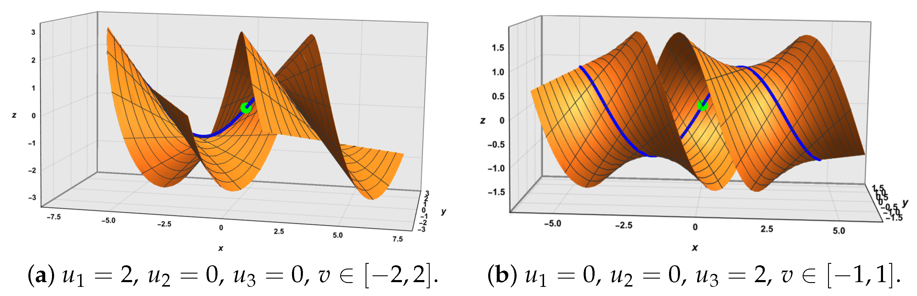
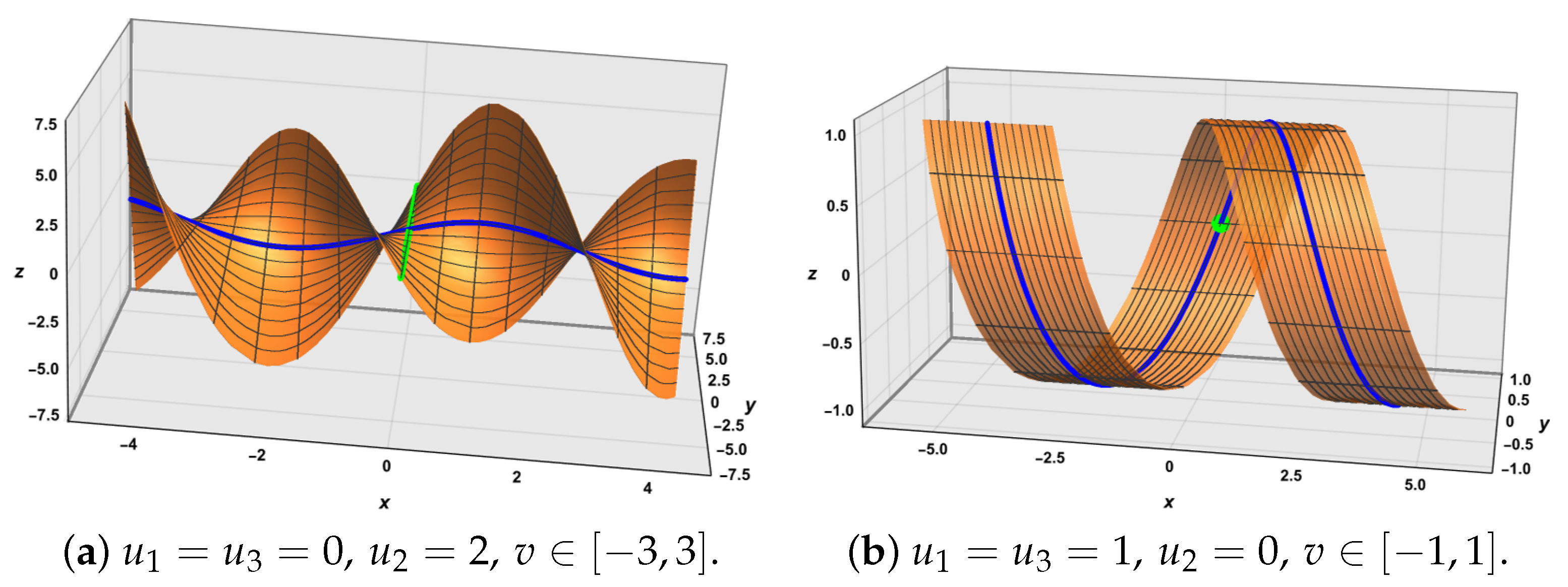
Figure 2.
The Ruled surface associated with a circular helix (the blue curve represents the base curve, the green point is a symmetric point, and the green line is a symmetric axis) for .
Figure 2.
The Ruled surface associated with a circular helix (the blue curve represents the base curve, the green point is a symmetric point, and the green line is a symmetric axis) for .
Disclaimer/Publisher’s Note: The statements, opinions and data contained in all publications are solely those of the individual author(s) and contributor(s) and not of MDPI and/or the editor(s). MDPI and/or the editor(s) disclaim responsibility for any injury to people or property resulting from any ideas, methods, instructions or products referred to in the content. |
© 2024 by the authors. Licensee MDPI, Basel, Switzerland. This article is an open access article distributed under the terms and conditions of the Creative Commons Attribution (CC BY) license (https://creativecommons.org/licenses/by/4.0/).
Share and Cite
MDPI and ACS Style
Gaber, S.; Sorour, A.H.; Abdel-Salam, A.A.
Construction of Ruled Surfaces from the W-Curves and Their Characterizations in
AMA Style
Gaber S, Sorour AH, Abdel-Salam AA.
Construction of Ruled Surfaces from the W-Curves and Their Characterizations in
Gaber, Samah, Adel H. Sorour, and A. A. Abdel-Salam.
2024. "Construction of Ruled Surfaces from the W-Curves and Their Characterizations in
Note that from the first issue of 2016, this journal uses article numbers instead of page numbers. See further details here.