Image Enhancement Based on Dual-Branch Generative Adversarial Network Combining Spatial and Frequency Domain Information for Imbalanced Fault Diagnosis of Rolling Bearing

Abstract

To address the problems of existing 2D image-based imbalanced fault diagnosis methods for rolling bearings, which generate images with inadequate texture details and color degradation, this paper proposes a novel image enhancement model based on a dual-branch generative adversarial network (GAN) combining spatial and frequency domain information for an imbalanced fault diagnosis of rolling bearing. Firstly, the original vibration signals are converted into 2D time–frequency (TF) images by a continuous wavelet transform, and a dual-branch GAN model with a symmetric structure is constructed. One branch utilizes an auxiliary classification GAN (ACGAN) to process the spatial information of the TF images, while the other employs a GAN with a frequency generator and a frequency discriminator to handle the frequency information of the input images after a fast Fourier transform. Then, a shuffle attention (SA) module based on an attention mechanism is integrated into the proposed model to improve the network’s expression ability and reduce the computational burden. Simultaneously, mean square error (MSE) is integrated into the loss functions of both generators to enhance the consistency of frequency information for the generated images. Additionally, a Wasserstein distance and gradient penalty are also incorporated into the losses of the two discriminators to prevent gradient vanishing and mode collapse. Under the supervision of the frequency WGAN-GP branch, an ACWGAN-GP can generate high-quality fault samples to balance the dataset. Finally, the balanced dataset is utilized to train the auxiliary classifier to achieve fault diagnosis. The effectiveness of the proposed method is validated by two rolling bearing datasets. When the imbalanced ratios of the four datasets are 0.5, 0.2, 0.1, and 0.05, respectively, their average classification accuracy reaches 99.35% on the CWRU bearing dataset. Meanwhile, the average classification accuracy reaches 96.62% on the MFS bearing dataset.

1. Introduction

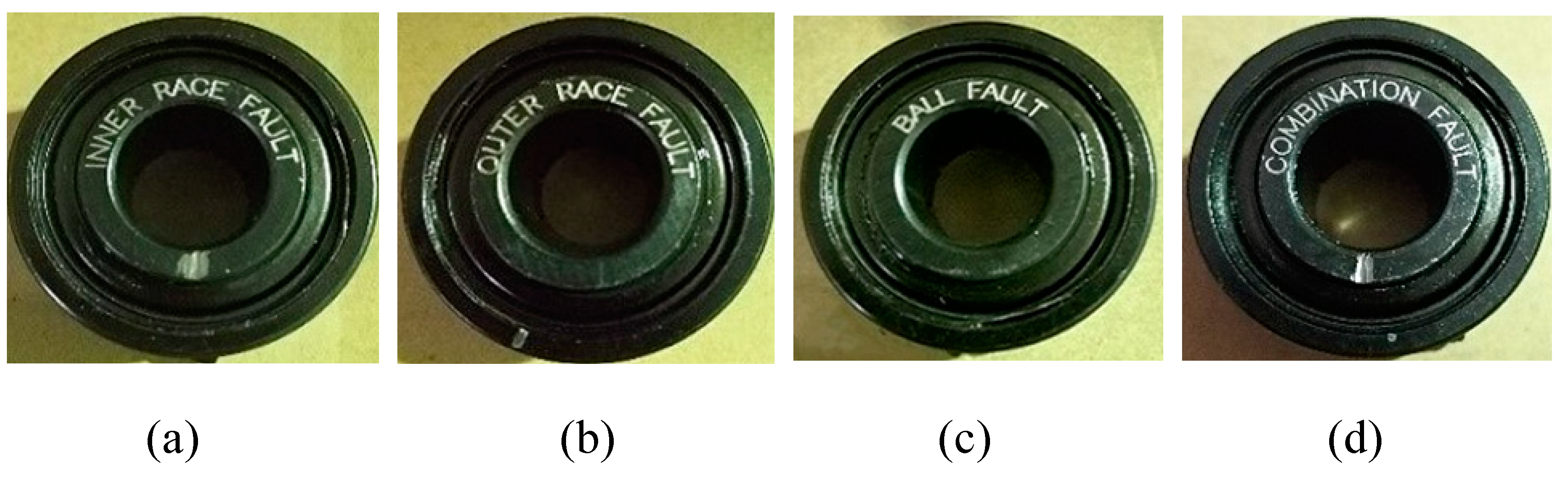
With the emergence of industry 4.0, the significance of mechanical equipment in modern industrial technology has become increasingly prominent. As a symmetry device, the rolling bearing is a crucial component in mechanical equipment and plays a vital role in ensuring the efficient and stable operation of such equipment [1]. Due to the long-term impact of thermal fatigue, alternating loads, mechanical vibration, wear, and other factors, it is also one of the most vulnerable mechanical components of mechanical equipment. Common types of faults include spalling, pitting, and wear. According to relevant statistics, the annual fault rate of rolling bearings is approximately 35%. Among these faults, the predominant issues are with the inner and outer rings and rolling bodies, accounting for about 90% [2]. Once the rolling bearing fails, it will affect the reliability of the mechanical equipment, and even lead to catastrophic consequences. Therefore, studying the fault diagnosis methods of the rolling bearing is essential to ensure mechanical equipment’s accuracy, reliability, and safety and to extend its service life [3,4].

Common fault diagnosis techniques for rolling bearings include methods based on vibration, sound, electrical, and temperature signals, among others. Among these, methods based on vibration signals are the most commonly used. Scholars have extensively researched methods for fault diagnosis in rolling bearings. In traditional fault diagnosis methods, qualitative approaches tend to be relatively imprecise and contain redundant information, and may lead to non-unique diagnosis results [5]. Methods that rely on semi-quantitative information can have significant errors. Diagnosis methods that rely on analytical models require precise parameters for the dynamic modeling of rolling bearings. However, due to the complex working environment and the difficulty in identifying fault mechanisms, the applicability of this method is limited.

In recent years, machine learning, especially deep learning, has been extensively utilized in monitoring bearing conditions and diagnosing faults in rotating machinery [6,7,8]. Compared to traditional methods that rely on manual feature extraction, deep learning models have potent capabilities for extracting features at a deep level and have achieved tremendous success in the latest applications for machine state monitoring and fault diagnosis [9,10]. For instance, Qiao et al. [11] utilized deep convolutional and LSTM recurrent neural networks to concurrently capture the temporal and frequency domain characteristics of vibration signals to achieve end-to-end fault diagnosis. Long et al. [12] proposed a multi-scale convolutional capsule network that integrates the multi-scale features extracted by a CNN with the spatial relationship features in CapsNet for the fault diagnosis of industrial robots. Huo et al. [13] presented an improved Adaptive Dimension Conversion–CNN approach for fault diagnosis. In this approach, 1D vibration signals were transformed into 2D matrices and then input into a 2D-CNN, fully leveraging the CNN’s ability to extract features from 2D data.

Data imbalance can significantly impact the stability and reliability of deep learning model training, leading to a substantial decrease in the performance of fault diagnosis models. Therefore, a significant amount of balanced data is crucial for training the deep diagnostic model to achieve accurate and reliable fault diagnosis results. However, in practical situations, mechanical equipment usually operates under normal working conditions, making it easy to collect sufficient operational data from the equipment under these conditions. On the contrary, mechanical equipment seldom operates under fault conditions, making it challenging to gather enough fault samples [14]. As a result, obtaining an extensive and balanced dataset to train deep learning models is difficult, significantly limiting the ability of deep learning models to achieve accurate fault diagnosis.

To solve the problem of imbalanced datasets in fault diagnosis, an increasing number of researchers have been investigating effective solutions [15,16]. For instance, Wu et al. [17] proposed a novel adaptive oversampling technique based on expectation maximization (EM) for local weighted minority oversampling in industrial fault diagnosis. Mao et al. [18] proposed a sequence prediction method based on an extreme learning machine to tackle the issue of imbalanced fault diagnosis, which incorporated the principal curve and granulation division to simulate the flow and overall distribution of fault data, effectively preserving the important features of fault samples. Shi et al. [19] proposed an undersampling technique that utilizes linear discriminant analysis and the gray wolf optimizer algorithm for threshold adjustment to improve the performance of fault classification.

However, the traditional methods mentioned above have a common drawback; they may generate incorrect or unnecessary samples and fail to increase the diversity of the original fault samples, resulting in issues such as overfitting and poor generalization ability, and only low diagnosis accuracy can be obtained.

In recent years, with the development of deep learning, the generative adversarial network (GAN) provides an alternative approach to addressing imbalanced fault diagnosis [20]. Originally used as a framework for generating images, the GAN has been proven to exhibit strong performance in image generation. However, the quality of the samples generated by the GAN is inferior due to unstable training. Therefore, to improve the performance of the GAN, an increasing number of models derived from the GAN have been proposed [21,22]. For example, to address the issue of data imbalance in practical industrial environments, Liu et al. [23] transformed 1D original vibration signals into 2D grayscale images and proposed an auxiliary classification GAN based on spectral normalization and gradient penalty. This GAN is employed to generate high-quality samples and incorporate them into the original dataset for data augmentation. Similarly, Fu et al. [24] proposed a small-sample data enhancement method for rotating machinery based on a fusion attention-guided Wasserstein GAN. This method reduces the multisensor data to three channels by principal component analysis, then converts the 1D data of each channel into a 2D pixel matrix and generates an RGB image by fusing the three-channel 2D image. Liu et al. [25] proposed an imbalanced fault diagnosis method based on an improved multi-scale residual GAN. By designing a multi-scale residual network structure and hybrid loss function, the original GAN model is improved, and high-quality time–frequency features are generated to balance fault data distribution. Xu et al. [26] proposed a semi-supervised conditional GAN with spectral normalization to generate time–frequency fault images with a similar distribution.

However, the existing imbalanced fault diagnosis methods based on the 2D time–frequency images mentioned above still face the following two drawbacks. (1) They all extract features from images in the spatial domain [27]. The images generated by these methods suffer from blurring, artifacts in texture details, and degradation of fake images compared to real images in terms of color. (2) They still suffer from inadequate extraction of local and global features. Although some models incorporate spatial or channel attention to overcome this deficiency [28,29], they do not consider the internal connection between these two types of attention, and are computationally complex, seriously affecting the reliability of diagnosis results.

The reasons for the limitations mentioned above are that the neural network tends to prioritize fitting the low-frequency components of the objective function when processing input images, especially as the network’s depth increases. On the other hand, the image’s texture details and color information are part of the high-frequency information, which the neural network does not prioritize fitting during training. Secondly, in the spatial domain, the color and brightness information of images are integrated through the intensity of pixel values in the three RGB channels. Therefore, processing the image in the spatial domain will impact the color information due to the lower brightness value. In contrast, in the frequency information domain, the image’s color information is primarily represented as high-frequency components, while the brightness information of the image is mainly represented as low-frequency components. Therefore, when processing the image in the frequency information domain, color and brightness are independent of each other, reducing interference between them.

Inspired by the above analysis, a novel data augmentation framework in which image enhancement based on a dual-branch GAN combining spatial and frequency domain information is established to improve the quality of the generated image. Meanwhile, the spatial domain information processing branch utilizes an auxiliary classification generative adversarial network (ACGAN) with a discriminator that can distinguish between true and false and realize fault diagnosis. The main contributions of this paper are summarized as follows:

(1)

A new dual-branch image enhancement GAN model combined with spatial and frequency domain information is proposed. Guided by the frequency domain GAN branch, the spatial domain ACGAN generates high-quality images with distinct texture details and vivid color. The generative capacity of this model significantly enhances the quality of the generated TF images, effectively addressing the data imbalance problem. Meanwhile, the auxiliary classifiers can achieve precise fault classification.

(2)

The shuffle attention [30] module based on spatial and channel attention mechanisms is integrated into the proposed model to form a pixel-level feature extraction network. The network is motivated to extract the local and global features of fault samples fully, enhancing the network’s expressive power. Compared to other attention modules, shuffle attention uses a parallel computation model, which makes it easier to focus on sensitive feature information and reduces computational complexity.

(3)

The Wasserstein distance and gradient penalty are incorporated into the loss function of the proposed model, significantly enhancing the data generation capability and solving the problems of gradient explosion and mode collapse during training.

The rest of this paper is organized as follows. We provide a brief introduction to the theory related to the GAN and its improved models in Section 2. We introduce the detailed structure and training method of the proposed model in Section 3. Section 4 discusses the experimental results and analysis of rolling bearing fault diagnosis. Finally, Section 5 summarizes the entire paper and gives a conclusion.

2. Basic Theory

In fault diagnosis tasks of rolling bearings, data imbalance often leads to overfitting and model instability, which reduces the accuracy and reliability of fault diagnosis. The generative adversarial network (GAN) is widely recognized as effective for generating high-quality images and data. Meanwhile, the GAN excels in learning and capturing complex data distributions, especially when dealing with imbalanced data. With the advancement of GAN technology, many variants have been proposed. These improved models offer better performance and generation results, making them more suitable for the imbalanced fault diagnosis of rolling bearings. Therefore, in this paper, GANs are employed to generate samples of specific fault categories to address the issue of data imbalance. This method can effectively enhance the quality of the generated data and fault diagnostic accuracy. Accordingly, the principles of the GAN and its derived models will be described in detail.

2.1. The GAN and Its Improved Models

The GAN [31] comprises a generator G and a discriminator D, which participate in a mutually antagonistic game. The decisions made by both sides of the game will combine to form a Nash equilibrium point, at which neither side will be able to increase their benefits through their behavior. During the training process, the generator constructs a mapping space P_z that satisfies the joint Gaussian distribution, gradually fitting the input noise z to the distribution P_r of real samples x to generate a new sample distribution P_g. The discriminator’s task is to receive true sample distribution P_r and the generated sample distribution P_g, and to distinguish between the authenticity of input samples. The ultimate objective is to identify the position that minimizes the losses of the generator and discriminator. The objective function of the entire process is as follows:

$$\underset{G}{\min } \underset{D}{\max }V(D,G)=E_{x\sim P_r(x)}[{\log }_{2}D(x)]+E_{z\sim P_z}[{\log }_2(1-D(G(z)))]$$

(1)

where E represents the expectation of the corresponding distribution, G(z) denotes the generated sample from generator, and D signifies the output of discriminator.

However, traditional GAN models suffer from defects such as training instability and mode collapse. The ACGAN [32] introduces conditional attribute information, which improves the model’s training stability and convergence speed while generating more diverse and attribute-specific samples. The loss function of the ACGAN includes discriminative loss and classification loss, and its general framework is shown in Figure 1. The discriminative loss function is as follows:

$$L_{dis}=E_{x\sim P_r(x)}[\log D(x,c_r)]+E_{z\sim P_z}[\log (1-D(G(z,c_g)))]$$

(2)

where x and c_r represent the real data and their respective category labels; c_g represents the label of the generated samples. c_g and z are input into generator G together to obtain the generated sample G(z, c_g), while D[G(z, c_g)] represents the probability that the discriminator D judges the generated G(z, c_g) to be true.

The classification loss function compels the generator to generate samples that align with the specified target category. The classification loss function is as follows:

$$L_{cls}^r=E_{x\sim P_r(x)}[-\log (P(c=c_r|x))]$$

(3)

$$L_{cls}^g=E_{z\sim P_z(z)}[-\log (P(c=c_g|G(z,c_g)))]$$

(4)

where P(c|x) represents the probability distribution of the category labels computed by the auxiliary classifier C.

In summary, the total loss functions during ACGAN training are as follows:

$$L_D=-L_{dis}+L_{cls}^r+L_{cls}^g$$

(5)

$$L_G=L_{dis}+L_{cls}^r+L_{cls}^g$$

(6)

During adversarial training, the discriminator needs to minimize L_D, and the generator needs to minimize L_G.

2.2. CWGAN-GP

The reliability of the ACGAN still needs to be improved because it uses JS divergence to distinguish the distance between the real distribution P_r and the fake distribution P_g. Furthermore, the JS divergence is discrete. When the two distributions of P_r and P_z do not overlap, the value of JS divergence remains a constant. This can make the model susceptible to gradient vanishing and mode collapse.

The CWGAN model is proposed to solve the problems mentioned above. It uses the Wasserstein distance to measure the discrepancy between these two distributions and can effectively address the limitations of the JS divergence. The Wasserstein distance is calculated as

$$W(P_r,P_z)=\underset{\gamma \sim \Pi (P_r,P_z)}{\inf }{E}_{(x,G(z))\sim \gamma }\left[\Vert x-G(z)\Vert \right]$$

(7)

where Π(P_r, P_z) represents the set of all possible joint distributions obtained by combining the true sample distribution P_r with the generated sample distribution P_z. For each possible joint distribution γ, one can sample (x, G(z))~γ from it to obtain samples x and G(z), and ǁx − G(z)ǁ represents the distance between the pairs of samples. Since it is impossible to solve for an exact lower bound on the Wasserstein distance directly, the Kantorovich–Rubinstein dual form is used. The Wasserstein distance is converted as

$$W(P_r,P_z)=\frac{1}{K}\underset{{\Vert f\Vert }_L\le K}{\sup }\left\{E_{x\sim P_r(x)}[f(x)]-E_{z\sim P(z)}[f(G(z))]\right\}$$

(8)

where sup is the minimum upper bound. f is a continuous function, ǁfǁ_L≤ K indicates that f must satisfy the Lipschitz continuity condition, and there exists a constant K ≥ 0 such that it meets |f(x) − f(G(z))| ≤ K|(x − G(z)| in the domain of definition. The objective function of the CWGAN is

$$\underset{G}{\min } \underset{D\in \Delta }{\max }V(G,D)=E_{x\sim P_r}[D(x|c)]-E_{z\sim P_z}[D(G(z|c))]$$

(9)

where Δ denotes the set of 1-Lipschitz functions. To implement the CWGAN, the discriminator D should belong to 1-Lipschitz functions, and it should satisfy condition |D(x) − D(G(z))| ≤ |x − G(z)|. To meet this requirement, the CWGAN truncates the discriminator D’s parameters at [−c, c] after each iteration.

However, this optimization strategy is susceptible to gradient explosion. To tackle this issue, Gulrajani et al. [33] proposed the gradient penalty term, which effectively solves the problem above by incorporating the gradient penalty term (GP) into the CWGAN. The objective function of the CWGAN-GP is as follows:

$$L_D=E_{z\sim P_z(z)}[D(G(z|c))]-E_{x\sim P_r(x)}[D(x|c)]+\lambda E_{\widehat{x}\sim P_{\widehat{x}}(\widehat{x})}\left[{({\Vert {\nabla }_{\widehat{x}}D(\widehat{x}|c)\Vert }_2-1)}^2\right]$$

(10)

$$L_G=-E_{z\sim P_z(z)}[D(G(z|c))]$$

(11)

$$\begin{array}{l}\widehat{x}=\epsilon x_r+(1-\epsilon )x_g,\\ x_r\in P_r,x_g\in P_z,\epsilon \in Uniform[0,1]\end{array}\}$$

(12)

where λ represents the gradient penalty weight, x_r and x_g represent the data in the real distribution P_r and the fake distribution P_z, $\widehat{x}$ is the data sampled by random interpolation of random noise on the line between x_r and x_g, $P_{\widehat{x}}(\widehat{x})$ represents the set of sampled data, ε represents the random number obeying the uniform distribution, and ${\Vert {\nabla }_{\widehat{x}}D(\widehat{x}|c)\Vert }_2$ represents the L₂-paradigm of the gradient of the D.

2.3. ACWGAN-GP

The ACWGAN-GP [34] effectively solves the shortcomings of traditional GAN models described above. It significantly enhances the reliability of GAN model training and improves the quality of the generated samples. The main idea is to use an ACGAN-based Wasserstein distance and evaluate the difference between the fake distribution and real distribution while employing a gradient penalty to satisfy the Lipschitz constraints. The loss function of the ACWGAN-GP is as follows:

$$\begin{array}{l}{L}_D=E_{x\sim P_r}[\log D(x,c_r)]-E_{z\sim P_z}[\log D(G(z,c_g))]-\lambda E_{\widehat{x}\sim P_{\widehat{x}}}\left[{({\Vert {\nabla }_{\widehat{x}}D(\widehat{x})\Vert }_2-1)}^2\right]\\ +E_{x\sim P_r}[\log P(Y=y|S_{real})]\end{array}$$

(13)

$$L_G=E_{z\sim P_z}[\log D(G(z,c_g))]+E_{z\sim P_z}[\log P(c=c_g|G(z,c_g))]$$

(14)

where P(Y = y|S_real) represents the probability distribution on the category labels.

In summary, the GAN possesses a powerful ability to generate high-quality images and data samples. However, its training process often encounters instability issues, such as gradient vanishing and mode collapse, compromising its robustness in practical applications. To address these challenges, researchers have proposed various enhancement methods. The ACGAN builds upon the original GAN by introducing conditional attribute information, leading to more diverse and attribute-specific generated samples. Nonetheless, it remains susceptible to gradient vanishing, and the model’s performance requires further optimization. The CWGAN-GP effectively addresses the issues of pattern collapse and gradient vanishing by incorporating the Wasserstein distance and gradient penalty terms. However, compared with the original GAN, the CWGAN-GP requires more training data to achieve enhanced generative capability and stability. The ACWGAN-GP combines the advantages of the ACGAN’s conditional attribute information and the CWGAN-GP’s training stability. Although its complexity increases the computational requirements, the ACWGAN-GP can generate high-quality samples with robust classification performance, positioning it as an excellent choice for imbalanced fault diagnosis of rolling bearing.

2.4. Continuous Wavelet Transform Feature Extraction

The continuous wavelet transform (CWT) [35] is widely used to extract the time and frequency domain features of the original vibration signals, the essence of which is to describe the original signal by translating and scaling the wavelet mother function; the time domain information of the signal is obtained by translating, and the frequency domain information of the signal is obtained by scaling the wavelet mother function. Wavelet analysis can locally amplify the time–frequency domain of the signal, adjust the scale factor, and change the time resolution of low-frequency and high-frequency signals and frequency resolution to adapt to the signals of different compositions, so the wavelet analysis method shows promising results in fault diagnosis, image processing, and other aspects.

Assuming the vibration signal is $s(t)\in L^2(R)$, the wavelet transform can be represented as follows:

$$c_s(a,b)=s\ast {\psi }_{a,b}(t)=\frac{1}{\sqrt{\left|a\right|}}{\displaystyle {\int }_{-\infty }^{\infty }s(t)}{\psi }_{a,b}\left(\frac{t-b}{a}\right)dt$$

(15)

where a b $\in$ R, a > 0 are the scaling and translation factors, respectively. ψ_a,b(⸱) is the scaling and translation factor. Analyzing the signal through the expansion of ψ(t) in the scale and the translation in the time domain, i.e., decomposing the existing time-domain signal into a two-dimensional time–frequency plane, is a TF domain analysis, which is more conducive to the extraction of local features of the original vibration signal. Generally, rolling bearing faults are always expressed as impulse shocks, whose shapes are similar to Morlet wavelets. Therefore, this paper uses a Morlet wavelet as the basis function to transform the original vibration signals into TF images with apparent local features.

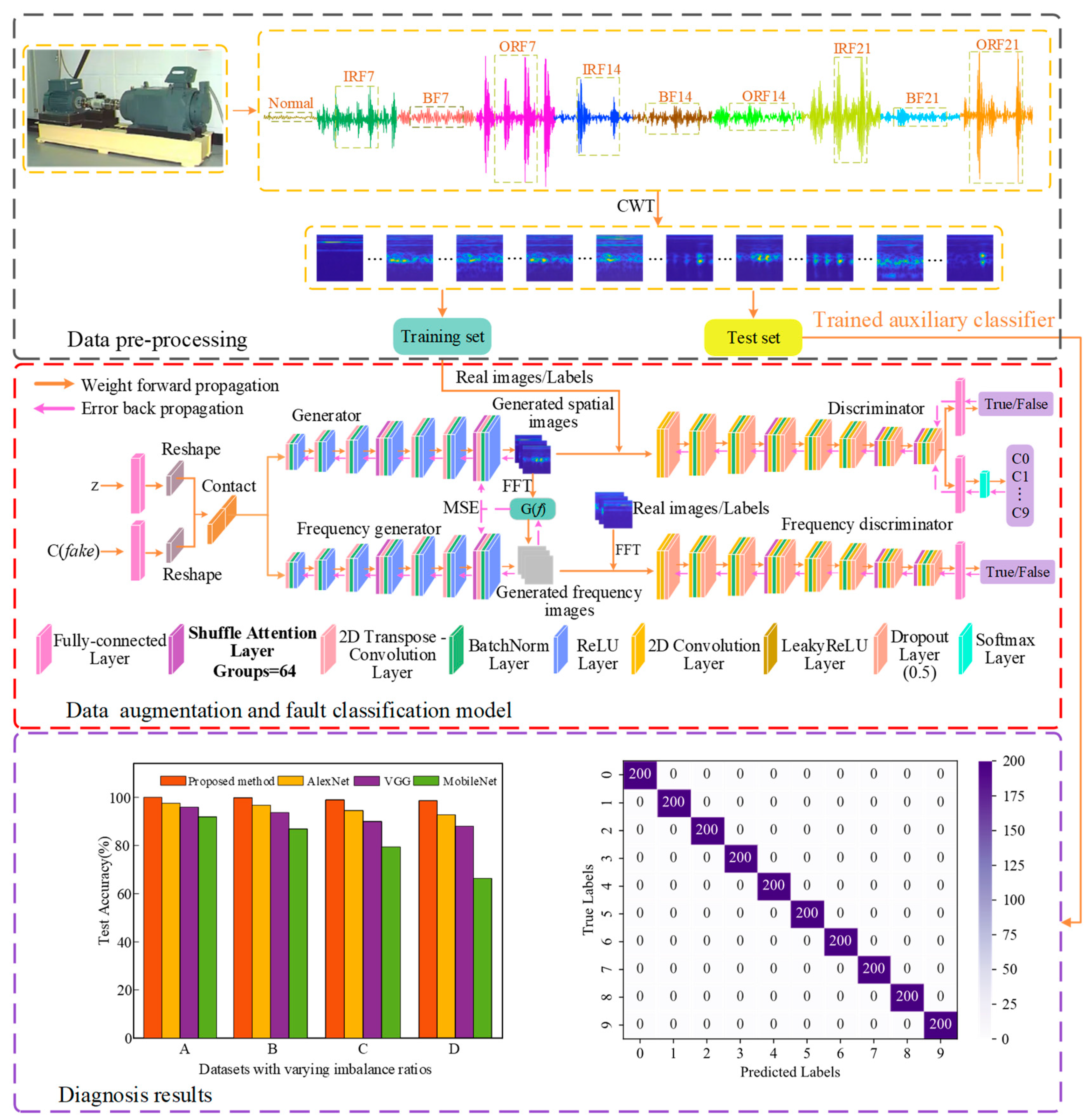
This paper employs the CWT to convert one-dimensional original vibration signals into two-dimensional time–frequency images, which are used as inputs to the proposed enhanced GAN model. Accordingly, the GAN’s excellent image generation capability is utilized to generate time–frequency images of specific fault categories and balance the original dataset.

3. The Proposed Method

In the spatial domain, images represent color and brightness information by combining intensity values across the three RGB channels. Low brightness values can affect the color information in TF images. Conversely, in the frequency domain, color and brightness information are represented by high-frequency and low-frequency components. Therefore, when dealing with TF images in the frequency domain, the color and brightness information are independent and do not interfere.

Based on the above problem and aiming at the problem of color distortion in images generated by existing 2D image-based GAN models for imbalanced fault diagnosis, this paper proposes a novel image enhancement model based on a dual-branch GAN combining spatial and frequency domain information. The overall flowchart of the proposed model is shown in Figure 2. The spatial domain information processing branch utilizes an auxiliary classification GAN, which comprises a generator (G) and a discriminator (D). Meanwhile, the frequency domain information processing branch uses a GAN with a frequency generator (FG) and a frequency discriminator (FD). A fast Fourier transform is used to transform the input image from the spatial domain to the frequency domain. The MSE is integrated into the loss function of both generators to enhance the consistency of frequency information for the generated images. Two of the GANs receive the same noise and labeling information and the ACWGAN-GP is responsible for generating high-quality image samples and balancing the original dataset. Finally, the auxiliary classifier is trained with a balanced dataset to achieve intelligent imbalanced fault diagnosis of the rolling bearing.

3.1. Fast Fourier Transform and Consistency Measure Mean Square Error Loss

3.1.1. Fast Fourier Transform

In image processing, the FFT is an effective method for separating the frequency information components of an image from the spatial domain [36]. Therefore, this paper utilizes the FFT to separate the frequency information of the input image from the spatial domain. The computational method of the FFT is defined as follows:

$$F(u,v)={\displaystyle \sum _{x=0}^{W-1}{\displaystyle \sum _{y=0}^{H-1}S(x,y)\cdot e^{-j2\pi (\frac{ux}{W}+\frac{vy}{H})}}}$$

(16)

where S(x, y) denotes the pixel value of the image at the spatial domain coordinate (x, y); H and W are the height and width of the image, respectively. After the FFT operation, the input image will get the spectrogram with the same size as H and W, which is the representation of the image in the frequency domain. The F(u, v) represents the frequency components’ intensity and phase information at the frequency domain’s spectral coordinates (u, v).

3.1.2. Consistency Measure Mean Square Error Loss

Consistency measure mean square error (MSE) is a commonly used statistical metric to measure the difference between the expected and actual values. It has a significant advantage in calculating the discrepancy in pixel values between two images [37]. The formula is defined as follows:

$$MSE=\frac{1}{N}{\displaystyle \sum _{i=1}^N{(y_i-h(x_i))}^2}$$

(17)

where y_i and x_i represent the actual and expected values of the ith frequency component, respectively, and N represents the total number of frequency components.

For the training loss of the proposed model, the discriminator loss function of the spatial domain generative model is kept consistent with the ACWGAN-GP mentioned above, according to the knowledge discussed in Section 2. At the same time, by introducing the MSE loss into the generator, the loss of the spatial domain generator network is as follows:

$$L_G=\alpha [-E_{z\sim P_z}[\log D(G(z,c_g))]+E_{z\sim P_z}[-\log P(c=c_g|G(z,c_g))]]+(1-\alpha )MSE$$

(18)

Accordingly, the frequency information branch using the CWGAN-GP and the loss function of the frequency generator is as follows:

$$L_G=-\alpha E_{z\sim P_z(z)}[D(G(z|c_g))]+(1-\alpha )MSE$$

(19)

where α is a hyperparameter to adjust the weight ratio between the two loss functions, and the α is set to 0.01 in this paper.

This paper introduces MSE loss in the two generators to evaluate the disparity between the frequency information of the spatial and frequency domain pseudo-images. The gradients of the loss functions of the two generators are updated during training to enhance the consistency of the frequency information for the generated images. Therefore, the frequency information branch can supervise the spatial information branch in learning the detailed texture features of images more comprehensively, allowing the G to generate fault images with a higher resolution.

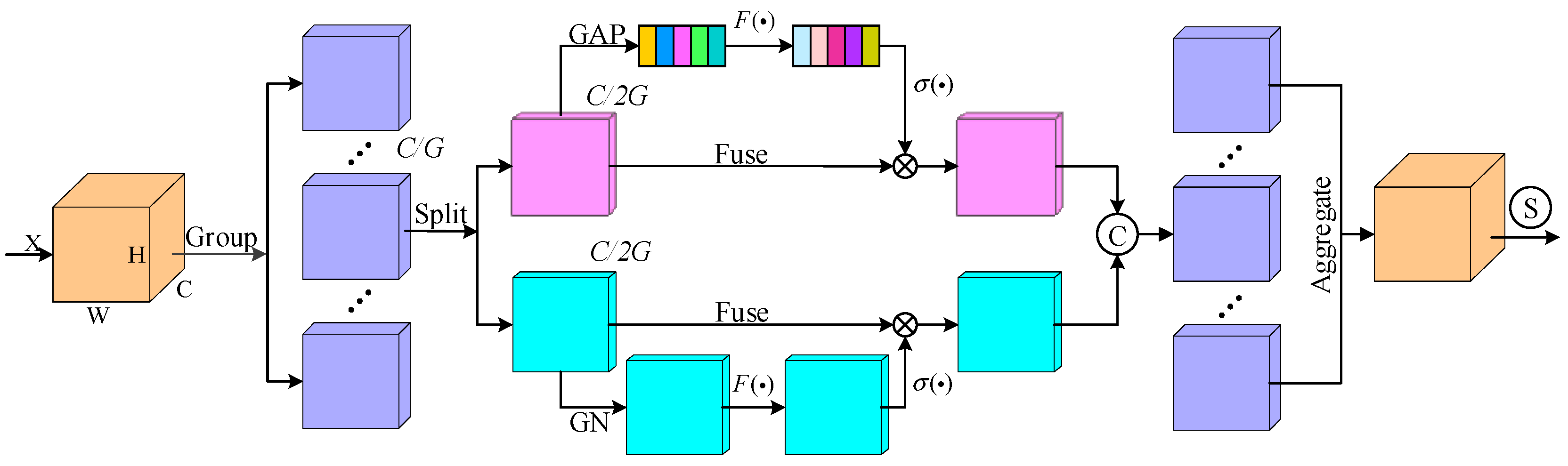
3.2. Shuffle Attention Module

Recently, the use of attention mechanisms in fault diagnosis has become increasingly widespread. Efficient channel attention (ECA) focuses on the intrinsic connections between pixel-level feature information. The convolutional block attention mechanism (CBAM) enables the model to focus on the spatial relationships of features and the intrinsic connection between channels by combining spatial and channel attention [38,39]. However, they do not adequately consider the intrinsic connection between spatial and channel attention mechanisms and still have limitations in terms of computational efficiency.

To enhance the expression ability of the proposed model and alleviate the computational burden caused by the dual GAN structure, the shuffle attention (SA) module is proposed, employing a parallel computation approach that enables the model to extract global feature information and reduce computational complexity significantly.

As shown in Figure 3, the input feature map is denoted as $X\in {ℝ}^{C\times H\times W}$, where C represents the number of channels, H represents the height, and W represents the width. Additionally, SA sets the value of G as the segmentation parameter. The input feature map X is divided into G sub-feature maps along the channel to form a branch, denoted as X = [X₁, …, X_G] and $X_k\in {ℝ}^{C\times H\times W/G}$. Each branch X_k is computed in parallel during the feature extraction process, enhancing computation speed and obtaining new weight parameters through the attention module in the feature extraction process. After each branch enters the attention module, X_k is further subdivided into two branches along the channel, denoted as X_k1, $X_{k2}\in {ℝ}^{C\times H\times W/2G}$; X_k1 and X_k2 form the preliminary channel attention feature map and spatial attention feature map through the feature information between channels and sub-feature maps, respectively. At this point, the model obtains the source information of different feature maps.

To enhance the integration of feature information between the channel attention and the spatial attention feature map, the overall feature information is extracted using global average pooling (GAP), denoted as $S\in {ℝ}^{C\times 1\times 1/2G}$, and X_k1 is recomputed using the overall feature information.

$$s=GAP(X_{k1})=\frac{1}{H\times W}{\displaystyle \sum _{i=1}^H{\displaystyle \sum _{j=1}^W{X}_{k1}(i,j)}}$$

(20)

The sigmoid activation function is utilized to regulate the fusion of the dual-channel feature information, and the final channel attention output is:

$${X^{\prime }}_{k1}=\sigma (F(s))\cdot X_{k1}=\sigma (W_{1}s+b_1)\cdot X_{k1}$$

(21)

where W₁ and $b_1\in {ℝ}^{C\times 1\times 1/2G}$ are the parameters used to rescale the output feature map.

Spatial attention focuses more on the source of information. After calculating the output of channel attention obtained by X_k1, it is also necessary to calculate the spatial attention of X_k2. This ensures that all feature information can be effectively obtained when the two branches are merged. The group norm (GN) is used for X_k2 to obtain the spatial features, and then the enhancement F(⸱) is applied. The final output of spatial attention is

$${X^{\prime }}_{k2}=\sigma (W_2\cdot GN(X_{k2})+b_2)\cdot X_{k2}$$

(22)

where W₂ and $b_2\in {ℝ}^{C\times 1\times 1/2G}$ merge the two attention feature map branches, denoted as X′_k = [X′_k1, X′_k2]$\in {ℝ}^{C\times H\times W/G}$, W₁, b₁, W₂, b₂, and the GN hyperparameters are generated in the SA module, and the number of channels in each branch is split by the G-parameter, ensuring that the SA is sufficiently lightweight. Finally, the shuffle operator is used to merge and flow the feature information of each branch along the channels across the branches, ensuring that the final output of the SA module is consistent with the size of X.

In summary, compared with other attention mechanisms, shuffle attention allows the input feature information to flow between different channels. This enables the effective capture of the relationship between global and local features in both spatial and frequency domains. In addition, it can perform both spatial and channel branching feature extraction, making it more computationally efficient and lightweight. Therefore, in this paper, shuffle attention is incorporated into the proposed model to enhance the feature extraction capability of the network while reducing the computational burden associated with the dual GAN structure.

3.3. Overall Flow of the Proposed Method

This paper aims to generate time–frequency images with sufficient texture details and color information to improve fault diagnosis accuracy. A dual-branch GAN model that combines information from both the spatial and frequency domains of images is proposed. The general flow of the proposed diagnosis method is shown in Figure 4. In the spatial domain generator, 100-dimensional noise and the label C (fake) are input into a fully connected (FC) layer. A reshape function transforms the FC layer’s output into 4 × 4 × 384 images. Then, seven feature extraction modules are employed, each containing a convolution layer, batch normalization, and ReLU activation function. The 4th and 7th feature extraction modules contain shuffle attention layers. The size of the image is altered by employing multiple 4 × 4 convolution kernels. The number of output channels of the last layer is 3, corresponding to the channels of the RGB image. Simultaneously, the discriminator consists of 8 feature extraction modules, and the input image size is 64 × 64 × 3. The shuffle attention layer is included in the 4th and 8th feature extraction modules. To enhance the discriminator’s performance, the LeakyReLU activation function is employed. The output layer constructs an auxiliary classifier using the softmax activation function to achieve fault learning and recognition. The detailed network parameters of G and D are shown in

Table 1. The specific network parameters of the generator and discriminator.

Network	Layer	Kernel	Strides	Maps	N	AF
Generator	Input (100, 10)	—	—	—	—	—
	Full connection	—	—	768	—	—
	Deconv2d	4 × 4	1 × 1	384	BN	ReLU
	Deconv2d	4 × 4	2 × 2	256	BN	ReLU
	Deconv2d	4 × 4	2 × 2	192	BN	ReLU
	Shuffle attention	—	—	192	—	—
	Deconv2d	4 × 4	2 × 2	64	BN	ReLU
	Deconv2d	4 × 4	2 × 2	64	BN	ReLU
	Deconv2d	4 × 4	2 × 2	64	BN	ReLU
	Shuffle attention	—	—	16	—	—
	Deconv2d	4 × 4	2 × 2	3	BN	Tanh
Discriminator	Input(64 × 64 × 3)	—	—	—	—	—
	Conv2d	3 × 3	2 × 2	16	—	LeakyReLU
	Conv2d	3 × 3	1 × 1	32	BN	LeakyReLU
	Conv2d	3 × 3	2 × 2	64	BN	LeakyReLU
	Shuffle attention	—	—	64	—	—
	Conv2d	3 × 3	1 × 1	128	BN	LeakyReLU
	Conv2d	3 × 3	2 × 2	256	BN	LeakyReLU
	Conv2d	3 × 3	1 × 1	512	BN	LeakyReLU
	Conv2d	3 × 3	2 × 2	512	BN	LeakyReLU
	Shuffle attention	—	—	512	—	—
	Conv2d	3 × 3	2 × 2	512	BN	LeakyReLU
	Full connection	—	—	1	—	sigmoid
	Full connection	—	—	10	—	softmax

Note: N and AF stand for “Normalization” and “Activation Function”, respectively. Maps represent the number of output channels.

. It is worth noting that the network parameters of the frequency domain WGAN-GP are the same as those of the spatial domain ACWGAN-GP, except that the last layer of the FG has only one output channel and does not include a fully connected layer with a softmax activation function.

The TF images are divided into a training set and a test set with a ratio of 4:1, and the balanced dataset is used to train the auxiliary classifier in the spatial discriminator. Then, the performance of the trained classifier is evaluated using the test set. During the training of the proposed model, the learning rates of the two sets of generators and discriminators are set to 0.0001 and 0.0002, respectively. The number of training iterations for the generative task is 500, while the number of training iterations for the auxiliary classifier is 200, and the batch size is 32. Adam’s algorithm is used as the optimizer for this model, with momentum parameters β₁ and β₂ set to 0.5 and 0.999, respectively. The model also utilizes LeakyReLU and Dropout with parameters of 0.2 and 0.5, and the value of the gradient penalty coefficient λ is 5.

4. Experimental Verification

To comprehensively confirm the validity of the proposed method, we conducted detailed experiments on two bearing datasets. The rolling bearing dataset for case 1 was obtained from the Case Western Reserve University (CWRU) bearing data center. The dataset for case 2 was obtained from the Mechanical Fault Simulation Platform (MFS). The experiment was conducted on a computer running the 64-bit Windows 10 operating system. The hardware configuration included an Intel(R) Core (TM) i5-13490F CPU, an NVIDIA GeForce RTX3060Ti GPU, 32GB of RAM, Python 3.9.15, and PyTorch 1.13.1.

4.1. Case 1: The Case Western Reserve University (CWRU) Bearing Dataset

4.1.1. Description of The Dataset

The bearing dataset from CWRU is a well-recognized standard dataset in bearing fault diagnosis and is widely used in related research and practice. The experimental platform included a 2-horsepower motor, torque sensor and decoder, power tester, and electronic control equipment. Single-point damage faults were created on the outer raceway, inner raceway, and balls of the bearing using electrical discharge machining (EDM).

The damage diameters were 0.007, 0.014, and 0.021 inches, respectively. To collect vibration signals from various fault categories, the experimental data selected for this study are as follows; a vibration acceleration sensor with a sampling frequency of 12 kHz, a motor load of 0 hp, and a motor speed of 1797 rpm were chosen. The damage diameters of the fault samples were 0.007, 0.014, and 0.021 inches. The fault locations were identified as follows: outer raceway of the bearing (outer fault), inner raceway of the bearing (inner fault), and the ball (ball fault), resulting in a total of nine types of fault data. These were combined with the normal bearing vibration data, resulting in a total of ten types of samples. They are marked from 0 to 9 in order and denoted as Normal, BF7, BF14, BF21, IRF7, IRF14, IRF21, ORF7, ORF14, and ORF21 in that sequence.

4.1.2. Dataset Setting

The original vibration signal for each fault contained 120,000 sample points, with each fault sample consisting of 600 sampling points. To increase the number of training samples while maintaining sample diversity [40], a 120-point interval was used for overlapping samples. The original vibration signal of each fault was converted into 1000 TF images by CWT, including 800 training samples and 200 test samples.

To simulate the imbalance of datasets in practical engineering, the TF images were randomly segmented and reorganized into five datasets. Dataset E is a fully balanced dataset for evaluating the classifier’s performance. A, B, C, and D are distributed with imbalanced ratios of 2:1, 5:1, 10:1, and 20:1 between the number of normal and faulty samples for each category, respectively. The proposed generative model in this paper was first utilized to generate class-specific fault samples to balance the four datasets. Subsequently, the balanced datasets A′, B′, C′, and D′ were employed to train the auxiliary classifier in the spatial discriminator. Finally, the dataset E was utilized as a test set to assess the diagnostic accuracy of the different balanced datasets. The number of samples for specific fault categories is shown in

Table 2. The detailed division of the CWRU rolling bearing dataset.

State	Normal	Ball Fault	Inner Fault	Outer Fault
Fault Diameter (inches)	0	0.007/0.014/0.021	0.007/0.014/0.021	0.007/0.014/0.021
Dataset A	800	400/400/400	400/400/400	400/400/400
Dataset B	800	160/160/160	160/160/160	160/160/160
Dataset C	800	80/80/80	80/80/80	80/80/80
Dataset D	800	40/40/40	40/40/40	40/40/40
Dataset E	200	200/200/200	200/200/200	200/200/200

.

4.1.3. Quality Assessment of Generated Images

To verify the capability of the proposed model to generate high-quality images with clear texture details and rich colors, a qualitative visual comparison was conducted between the proposed model and the CWGAN-GP, a widely used data enhancement model known for its excellence. As shown in Figure 5, it is evident that CWGAN-GP effectively generates the important features of faults and exhibits high visual quality. However, it still suffers from spectral inhomogeneity and lacks sufficient local detailed features. In contrast, the images generated by the proposed method have more apparent texture details and color information.

The structural similarity index (SSIM) was designed based on the visual perceptual properties of images, integrating the three aspects of brightness, contrast, and structure. It is suitable for objectively assessing image quality in image processing. By utilizing the Inception model to extract image features, the Fréchet inception distance (FID) can sensitively capture subtle differences between images, making it particularly effective for quality assessments of the generated images. Peak signal-to-noise ratio (PSNR) is a straightforward and intuitive image quality assessment method that evaluates an image’s quality by calculating the maximum possible error between the original and processed images. It has a simple formula and is well-suited for scenarios where image quality needs to be assessed quickly. Therefore, to objectively evaluate the generative ability of the proposed method, this paper uses SSIM, FID, and PSNR metrics to quantitatively evaluate the similarity between the generated and the original images. As shown in

Table 3. Mean values of the metrics for the original samples and generated samples on the CWRU datasets.

Datasets	SSIM	FID	PSNR
A	0.883	58.893	29.150
B	0.876	59.215	29.086
C	0.824	61.329	28.592
D	0.813	64.092	26.757

, in each of these four imbalanced datasets, the mean SSIM value for the ten categories of fault images exceeds 0.8, the mean FID values are around 60, and the mean PSNR values are around 29. These results indicate that the discrepancy between the fake and original distributions is minimal, and the generated images are of high quality.

To fully demonstrate the ability of the proposed method to generate high-quality TF images, we compare the evaluation metrics with existing generative models such as the DCGAN, ACGAN, and CWGAN-GP on dataset A. It is worth noting that the hyperparameters are consistent across all models, ensuring a fair comparison.

Table 4. Performance comparison of different data enhancement models.

Methods	SSIM	FID	PSNR
DCGAN	0.621	108.031	21.364
ACGAN	0.639	106.165	21.962
CWGAN-GP	0.743	71.027	24.425
The proposed method	0.883	58.893	29.150

presents the results of the comparison of their generative abilities. From the comparison, the generative ability of the DCGAN is significantly inferior, while the ACGAN and CWGAN-GP are relatively superior. However, the proposed method achieves optimal performance in all key metrics compared to these three models. Specifically, it achieves a mean SSIM value of 0.883, while the mean PSNR value is 29.150, indicating that the generated TF images are highly similar to the original images. The comparison results confirm that the proposed model possesses excellent image generation capability and provides more reliable input samples for fault classification.

4.1.4. Experiment Results

After the auxiliary classifier completed training on these four balanced datasets A′, B′, C′, and D′, the test set E was used to assess the reliability of the training results. The four confusion matrices depicting the classification results of the test set E are shown in Figure 6. This visual representation intuitively illustrates the accuracy of fault classification. The rows and columns of the confusion matrix represent the actual labels of the fault categories and the predicted labels, respectively. It can be noted that with an imbalance ratio of 2:1, the classification accuracy reaches 100%. At the imbalance ratio of 5:1, only one of the samples with fault categories BF7 and BF14 was misclassified, and only two of the fault samples with fault category IRF7 were misclassified. Meanwhile, only around 5% of the samples in the IR7 category were misclassified when the imbalance ratio is 20:1. These results demonstrate the effectiveness of the proposed method in enhancing the original dataset, enabling the ACWGAN-GP network to effectively capture the characteristic distribution of fault samples.

Figure 6. Confusion matrix of classification results for the CWRU datasets with different imbalance ratios.To further illustrate the feature learning performance of the proposed diagnostic model with various unbalanced datasets, we utilized the t-distributed stochastic neighbor embedding (t-SNE) algorithm [41] to visualize the classification results of the model on the test set. As shown in Figure 7, it is evident that the feature distributions of the test set samples with different health states in the four datasets exhibit significant differences. Although there are a few samples with conflated feature distributions, this impact on the model’s diagnosis results can be largely disregarded. This further validates the confusion matrices’ classification results and underscores the proposed model’s excellent feature learning and fault diagnosis capability.

Figure 6. Confusion matrix of classification results for the CWRU datasets with different imbalance ratios.To further illustrate the feature learning performance of the proposed diagnostic model with various unbalanced datasets, we utilized the t-distributed stochastic neighbor embedding (t-SNE) algorithm [41] to visualize the classification results of the model on the test set. As shown in Figure 7, it is evident that the feature distributions of the test set samples with different health states in the four datasets exhibit significant differences. Although there are a few samples with conflated feature distributions, this impact on the model’s diagnosis results can be largely disregarded. This further validates the confusion matrices’ classification results and underscores the proposed model’s excellent feature learning and fault diagnosis capability.

Figure 7. The visualization of t-SNE for classification results on the CWRU datasets with different imbalance ratios.

Figure 7. The visualization of t-SNE for classification results on the CWRU datasets with different imbalance ratios.

4.1.5. Comparison of Different Diagnosis Models

To further verify the diagnostic performance of the proposed model, the classification results of the model were compared with those of different models, including AlexNet, MobileNet, and VGG, at four different imbalance ratios. Their number of training iterations was set to 200, and the learning rate was fixed at 0.0002. The Adam optimization algorithm was also applied to the three comparison diagnostic models, and all hyperparameters remained consistent with those of the proposed models. Five experiments were conducted for each method to minimize random errors, and their average value was calculated. The diagnostic accuracies of various models are shown in Figure 8. It is evident that MobileNet has the poorest results, with classification accuracies of only 79.40% and 66.35% in datasets C and D, respectively. In contrast, AlexNet and VGG show significant improvements in classification accuracy across the four datasets. It is worth noting that the proposed model has the highest diagnostic accuracy among all models in the four datasets. Even in the case of an imbalanced ratio of 20:1, the diagnostic accuracy of the proposed model still reaches 98.65%, indicating the model has excellent feature extraction capability.

4.2. Case 2: Mechanical Fault Simulation (MFS) Platform Bearing Dataset

4.2.1. Description of the Dataset

To further verify the strong performance and generalization capability of the proposed model, the Mechanical Fault Comprehensive Simulation Platform from the laboratory was utilized. As shown in Figure 9, the experimental platform consisted of an AC motor, a coupling, an acceleration sensor, a rotor, an experimental bearing, an alignment adjustment plate, an inverter, and a data acquisition box, and the motor speed was 1000 rpm. As shown in Figure 10, the experiment collects bearing data from five fault states at a sampling frequency of 16 kHz. These states include the normal state and four fault states labeled from 0 to 4, representing normal, inner race fault (IRF), outer race fault (ORF), ball fault (BF), and combination fault (CF), in that order.

4.2.2. Dataset Setting

Similar to case 1, four datasets (A, B, C, and D) with different imbalance ratios of 2:1, 5:1, 10:1, and 20:1, respectively, were established. Additionally, dataset E, a fully balanced dataset, was used as a test set, and the detailed division of the datasets is shown in

Table 5. The detailed division of the MFS bearing dataset.

State	Normal	IRF	CF	ORF	BF
Dataset A	500	250	250	250	250
Dataset B	500	100	100	100	100
Dataset C	500	50	50	50	50
Dataset D	500	25	25	25	25
Dataset E	125	125	125	125	125

.

4.2.3. Quality Assessment of Generated Images

Similar to case 1, the generated images for each category were quantitatively compared with the original images using SSIM, FID, and PSNR, and the average of the comparison results for all fault categories was calculated and is shown in

Table 6. Mean values of the metrics for the original samples and generated samples on the MFS datasets.

Datasets	SSIM	FID	PSNR
A	0.840	59.994	28.882
B	0.827	60.146	28.630
C	0.793	64.230	26.080
D	0.774	65.720	25.154

; it is evident that all three metrics show excellent results across various datasets, indicating a low level of distortion and further demonstrating the excellent image generative capacity of the proposed model.

4.2.4. Experimental Results

After completing the training of the auxiliary classifier using balanced datasets, the test set E was employed to assess the reliability of the classifier. Confusion matrices illustrating the classification results of the four datasets on the test set are shown in Figure 11. It is evident that almost all fault categories can still be correctly classified, even with extreme data imbalance, demonstrating the exceptional capability of the proposed model in capturing fault features.

Figure 11. Confusion matrix of classification results for the MFS datasets with different imbalance ratios. To better evaluate the diagnostic performance of the proposed model in a more intuitive way, the t-SNE dimensionality reduction visualization results are shown in Figure 12. It is evident that each fault category still exhibits a distinct classification boundary, further indicating the excellent data generation and fault diagnosis performance of the proposed model, along with its strong generalization ability.

Figure 11. Confusion matrix of classification results for the MFS datasets with different imbalance ratios. To better evaluate the diagnostic performance of the proposed model in a more intuitive way, the t-SNE dimensionality reduction visualization results are shown in Figure 12. It is evident that each fault category still exhibits a distinct classification boundary, further indicating the excellent data generation and fault diagnosis performance of the proposed model, along with its strong generalization ability.

Figure 12. The visualization of t-SNE for classification results on the MFS datasets with different imbalance ratios.

Figure 12. The visualization of t-SNE for classification results on the MFS datasets with different imbalance ratios.

4.2.5. Comparison of Different Diagnosis Models

To further validate the performance of the proposed diagnostic model, we compare its classification results on the test set with existing state-of-the-art deep learning models, including AlexNet, VGG, and MobileNet. As shown in Figure 13, it is evident that the proposed method achieves the highest classification accuracy across all four imbalance ratios. On the contrary, MobileNet exhibits the poorest performance among all the models, achieving only 46.50% accuracy in the unbalanced ratio of 20:1. This issue may be attributed to the low complexity of the MobileNet model, which fails to adequately capture the intricate features present in the dataset. Additionally, it may suffer from issues such as data imbalance or overfitting.

5. Conclusions

To address the issues of insufficient texture details and color distortion in the image generated by the existing image-based imbalanced fault diagnosis models, this paper proposes a novel image enhancement model based on a dual-branch GAN combining spatial and frequency domain information for imbalanced fault diagnosis of rolling bearing. First, the method applies a CWT to convert the 1D raw data into 2D time–frequency images. Then, a Wasserstein distance and gradient penalty are incorporated into the loss functions of the proposed model to prevent gradient vanishing and mode collapse. Therefore, in the proposed model, the spatial domain information processing branch employs an ACWGAN-GP, while a CWGAN-GP is applied to the frequency domain information processing branch after the fast Fourier transform. Subsequently, the MSE is integrated into the loss functions of both generators to enhance the consistency of frequency information for the generated image. SA is also incorporated into this model to alleviate the computational load resulting from the dual GAN structure and enhance the expression ability of the network. Under the supervision of the frequency domain information processing branch, the ACWGAN-GP generates high-quality TF images and balances the original dataset. Finally, the auxiliary classifier is used to train the balanced dataset for comprehensive feature extraction and accurate fault diagnosis.

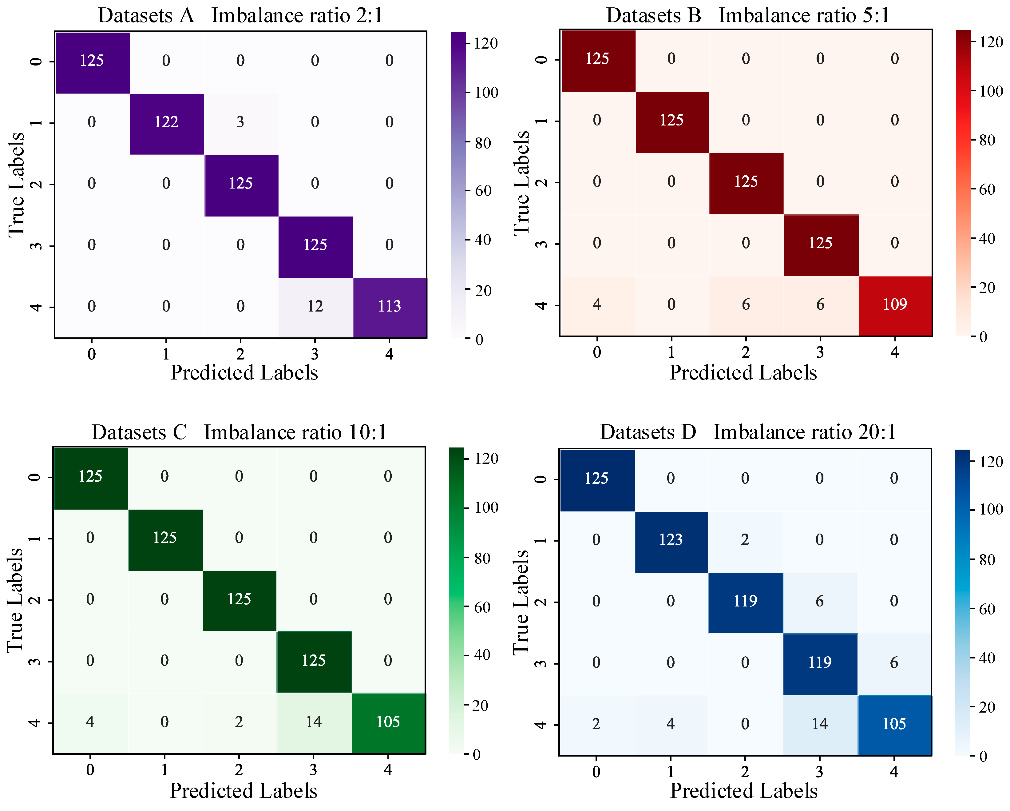
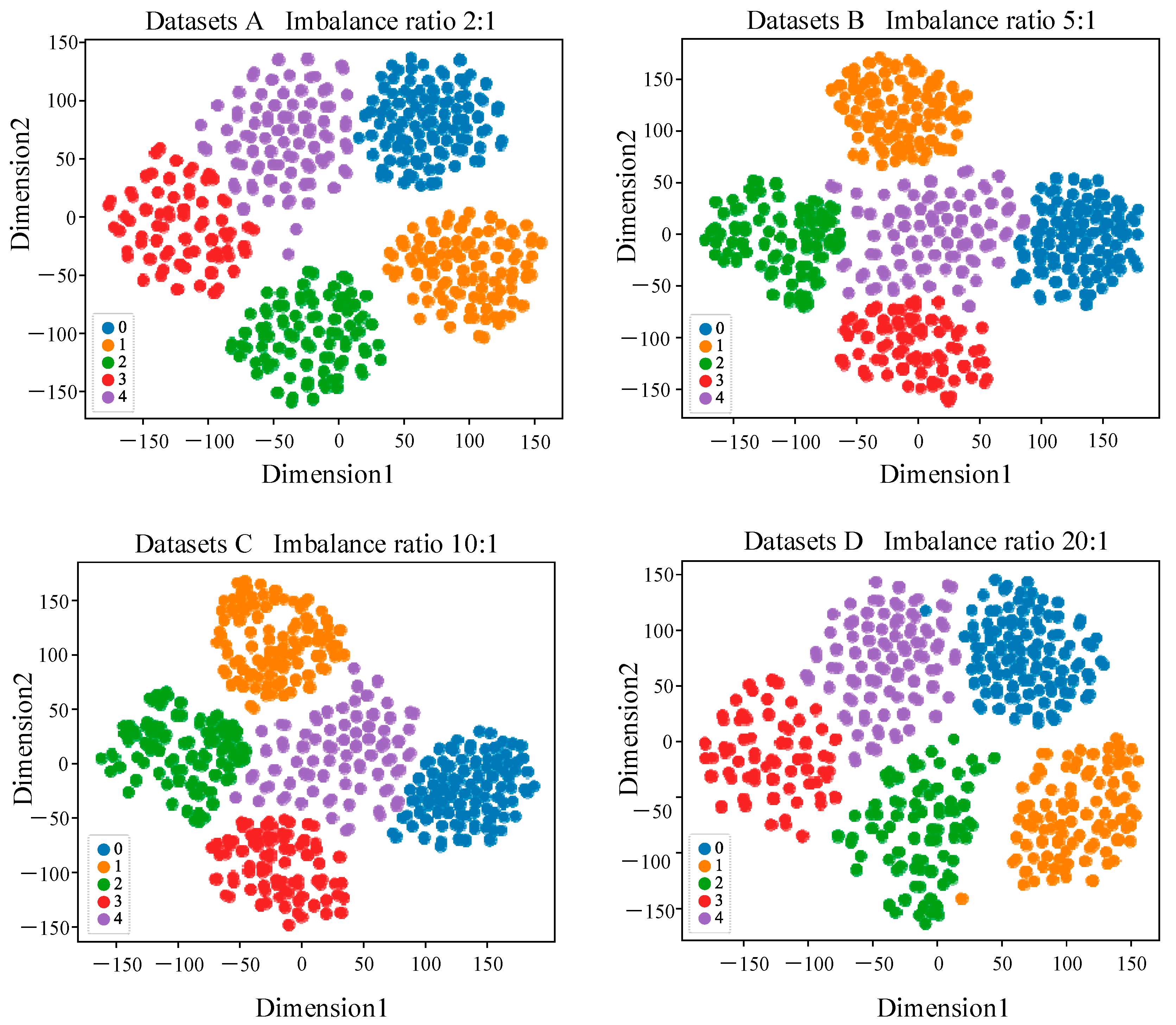
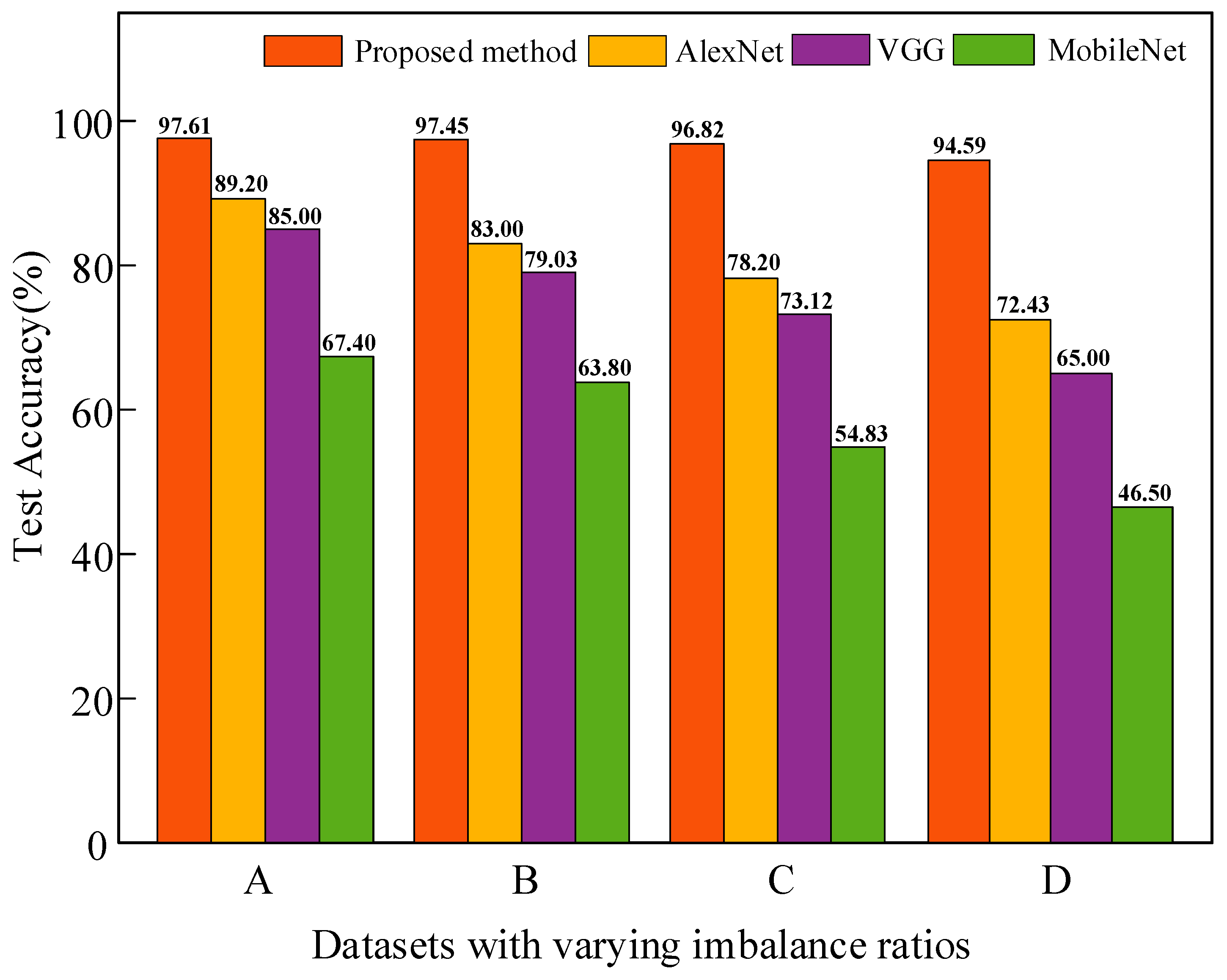
Experimental results on two bearing datasets indicate the high feasibility of the proposed method in both theory and practice. By comparing the performance with the existing state-of-the-art generative models, the results indicate that this method can generate higher-quality images with more apparent texture details and color information and enhance fault diagnosis performance and generalization ability. In addition, comparing the results of different diagnostic models indicates that the proposed method maintains high diagnosis accuracy on both datasets.

Although the integration of SA in the proposed model can alleviate the computational burden imposed by the dual GAN to some extent, the training of the proposed model is still time-consuming. Therefore, future research will further explore how to reduce the training time of the model more effectively and combine the frequency domain information of images with unsupervised learning. Furthermore, it is worth noting that the proposed method only applies to specific fault types and experimental subjects. Therefore, future work will incorporate transfer learning to diagnose more complex fault classes.

References

1. Wang, Z.; Yang, J.; Guo, Y. Unknown fault feature extraction of rolling bearings under variable speed conditions based on statistical complexity measures. Mech. Syst. Signal Process. 2022, 172, 108964. [Google Scholar] [CrossRef]
2. Fu, W.; Jiang, X.; Li, B.; Tan, C.; Chen, B.; Chen, X. Rolling bearing fault diagnosis based on 2D time-frequency images and data augmentation technique. Meas. Sci. Technol. 2023, 34, 045005. [Google Scholar] [CrossRef]
3. Xu, X.; Yu, Z. Failure analysis of tapered roller bearing inner rings used in heavy truck. Eng. Fail. Anal. 2020, 111, 104474. [Google Scholar] [CrossRef]
4. Wang, L.; Shao, Y. Fault feature extraction of rotating machinery using a reweighted complete ensemble empirical mode decomposition with adaptive noise and demodulation analysis. Mech. Syst. Signal Process. 2020, 138, 106545. [Google Scholar] [CrossRef]
5. Zhao, Z.; Chen, F.; Gui, Z.; Liu, D.; Yang, J. Refined composite hierarchical multiscale Lempel-Ziv complexity: A quantitative diagnostic method of multi-feature fusion for rotating energy devices. Renew. Energy 2023, 218, 119310. [Google Scholar] [CrossRef]
6. Lei, Y.; Yang, B.; Jiang, X.; Jia, F.; Li, N.; Nandi, A.K. Applications of machine learning to machine fault diagnosis: A review and roadmap. Mech. Syst. Signal Process. 2020, 138, 106587. [Google Scholar] [CrossRef]
7. Sun, J.; Yan, C.; Wen, J. Intelligent bearing fault diagnosis method combining compressed data acquisition and deep learning. IEEE Trans. Instrum. Meas. 2017, 67, 185–195. [Google Scholar] [CrossRef]
8. Liao, W.; Fu, W.; Yang, K.; Tan, C.; Huang, Y. Multi-scale residual neural network with enhanced gated recurrent unit for fault diagnosis of rolling bearing. Meas. Sci. Technol. 2024, 35, 056114. [Google Scholar] [CrossRef]
9. Li, X.; Jiang, H.; Niu, M.; Wang, R. An enhanced selective ensemble deep learning method for rolling bearing fault diagnosis with beetle antennae search algorithm. Mech. Syst. Signal Process. 2020, 142, 106752. [Google Scholar] [CrossRef]
10. Cao, H.; Shao, H.; Zhong, X.; Deng, Q.; Yang, X.; Xuan, J. Unsupervised domain-share CNN for machine fault transfer diagnosis from steady speeds to time-varying speeds. J. Manuf. Syst. 2022, 62, 186–198. [Google Scholar] [CrossRef]
11. Qiao, M.; Yan, S.; Tang, X.; Xu, C. Deep convolutional and LSTM recurrent neural networks for rolling bearing fault diagnosis under strong noises and variable loads. IEEE Access 2020, 8, 66257–66269. [Google Scholar] [CrossRef]
12. Long, J.; Qin, Y.; Yang, Z.; Huang, Y.; Li, C. Discriminative feature learning using a multiscale convolutional capsule network from attitude data for fault diagnosis of industrial robots. Mech. Syst. Signal Process. 2023, 182, 109569. [Google Scholar] [CrossRef]
13. Huo, C.; Jiang, Q.; Shen, Y.; Qian, C.; Zhang, Q. New transfer learning fault diagnosis method of rolling bearing based on ADC-CNN and LATL under variable conditions. Measurement 2022, 188, 110587. [Google Scholar] [CrossRef]
14. Jia, S.; Deng, Y.; Lv, J.; Du, S.; Xie, Z. Joint distribution adaptation with diverse feature aggregation: A new transfer learning framework for bearing diagnosis across different machines. Measurement 2022, 187, 110332. [Google Scholar] [CrossRef]
15. Zheng, T.; Song, L.; Guo, B.; Liang, H.; Guo, L. An efficient method based on conditional generative adversarial networks for imbalanced fault diagnosis of rolling bearing. In Proceedings of the 2019 Prognostics and System Health Management Conference (PHM-Qingdao), Qingdao, China, 25–27 October 2019; pp. 1–8. [Google Scholar]
16. Mao, W.; Liu, Y.; Ding, L.; Li, Y. Imbalanced fault diagnosis of rolling bearing based on generative adversarial network: A comparative study. IEEE Access 2019, 7, 9515–9530. [Google Scholar] [CrossRef]
17. Wu, Z.; Lin, W.; Fu, B.; Guo, J.; Ji, Y.; Pecht, M. A local adaptive minority selection and oversampling method for class-imbalanced fault diagnostics in industrial systems. IEEE Trans. Reliab. 2019, 69, 1195–1206. [Google Scholar] [CrossRef]
18. Mao, W.; He, L.; Yan, Y.; Wang, J. Online sequential prediction of bearings imbalanced fault diagnosis by extreme learning machine. Mech. Syst. Signal Process. 2017, 83, 450–473. [Google Scholar] [CrossRef]
19. Shi, Q.; Zhang, H. Fault diagnosis of an autonomous vehicle with an improved SVM algorithm subject to unbalanced datasets. IEEE Trans. Ind. Electron. 2020, 68, 6248–6256. [Google Scholar] [CrossRef]
20. Zhang, W.; Li, X.; Jia, X.D.; Ma, H.; Luo, Z.; Li, X. Machinery fault diagnosis with imbalanced data using deep generative adversarial networks. Measurement 2020, 152, 107377. [Google Scholar] [CrossRef]
21. Gao, X.; Deng, F.; Yue, X. Data augmentation in fault diagnosis based on the Wasserstein generative adversarial network with gradient penalty. Neurocomputing 2020, 396, 487–494. [Google Scholar] [CrossRef]
22. Liao, W.; Yang, K.; Fu, W.; Tan, C.; Chen, B.J.; Shan, Y. A Review: The Application of Generative Adversarial Network for Mechanical Fault Diagnosis. Meas. Sci. Technol. 2024, 35, 062002. [Google Scholar] [CrossRef]
23. Liu, S.; Dou, L.; Jin, Q. Improved Generative Adversarial Network for Bearing Fault Diagnosis with Imbalanced Data. In Proceedings of the 2023 6th International Conference on Information Communication and Signal Processing (ICICSP), Xi’an, China, 23–25 September 2023; pp. 343–347. [Google Scholar]
24. Fu, W.; Yang, K.; Wen, B.; Shan, Y.; Li, S.; Zheng, B. Rotating Machinery Fault Diagnosis with Limited Multisensor Fusion Samples by Fused Attention-Guided Wasserstein GAN. Symmetry 2024, 16, 285. [Google Scholar] [CrossRef]
25. Liu, J.; Zhang, C.; Jiang, X. Imbalanced fault diagnosis of rolling bearing using improved MsR-GAN and feature enhancement-driven CapsNet. Mech. Syst. Signal Process. 2022, 168, 108664. [Google Scholar] [CrossRef]
26. Xu, M.; Wang, Y. An imbalanced fault diagnosis method for rolling bearing based on semi-supervised conditional generative adversarial network with spectral normalization. IEEE Access 2021, 9, 27736–27747. [Google Scholar] [CrossRef]
27. Liang, P.; Deng, C.; Wu, J.; Yang, Z. Intelligent fault diagnosis of rotating machinery via wavelet transform, generative adversarial nets and convolutional neural network. Measurement 2020, 159, 107768. [Google Scholar] [CrossRef]
28. Meng, Z.; Li, Q.; Sun, D.; Cao, W.; Fan, F. An intelligent fault diagnosis method of small sample bearing based on improved auxiliary classification generative adversarial network. IEEE Sens. J. 2022, 22, 19543–19555. [Google Scholar] [CrossRef]
29. Peng, X.; Xu, H.; Wang, J.; Liu, J.; He, C. Ensemble multiple distinct ResNet networks with channel-attention mechanism for multi-sensor fault diagnosis of hydraulic systems. IEEE Sens. J. 2023, 23, 10706–10717. [Google Scholar] [CrossRef]
30. Hou, C.; Sun, Q.; Wang, W.; Zhang, J. Shuffle Attention Multiple Instances Learning for Breast Cancer Whole Slide Image Classification. In Proceedings of the 2022 IEEE International Conference on Image Processing (ICIP), Bordeaux, France, 16–19 October 2022; pp. 466–470. [Google Scholar]
31. Goodfellow, I.; Pouget-Abadie, J.; Mirza, M.; Xu, B.; Warde-Farley, D.; Ozair, S.; Courville, A.; Bengio, Y. Generative adversarial networks. Commun. ACM 2020, 63, 139–144. [Google Scholar] [CrossRef]
32. Wu, C.; Zeng, Z. A fault diagnosis method based on Auxiliary Classifier Generative Adversarial Network for rolling bearing. PLoS ONE 2021, 16, e0246905. [Google Scholar] [CrossRef]
33. Gulrajani, I.; Ahmed, F.; Arjovsky, M.; Dumoulin, V.; Courville, A.C. Improved training of wasserstein gans. Adv. Neural Inf. Process. Syst. 2017, 30. [Google Scholar]
34. Li, Z.; Zheng, T.; Wang, Y.; Cao, Z.; Guo, Z.; Fu, H. A novel method for imbalanced fault diagnosis of rotating machinery based on generative adversarial networks. IEEE Trans. Instrum. Meas. 2020, 70, 3500417. [Google Scholar] [CrossRef]
35. Yan, R.; Gao, R.; Chen, X. Wavelets for fault diagnosis of rotary machines: A review with applications. Signal Process. 2014, 96, 1–15. [Google Scholar] [CrossRef]
36. Nam, J.; Lee, S. Frequency filtering for data augmentation in X-ray image classification. In Proceedings of the 2021 IEEE International Conference on Image Processing (ICIP), Anchorage, AK, USA, 19–22 September 2021; pp. 81–85. [Google Scholar]
37. Pu, Y.; Wang, W.; Xu, Q. Image change detection based on the minimum mean square error. In Proceedings of the 2012 Fifth International Joint Conference on Computational Sciences and Optimization, Harbin, China, 23–26 June 2012; pp. 367–371. [Google Scholar]
38. Liang, X.; Guo, L. Fault diagnosis of batch process based on improved time convolution network and efficient channel attention. In Proceedings of the 2022 4th International Conference on Intelligent Information Processing (IIP), Guangzhou, China, 14–16 October 2022; pp. 129–133. [Google Scholar]
39. Chang, M.; Yao, D.; Yang, J. Intelligent Fault Diagnosis of Rolling Bearings Using Efficient and Lightweight ResNet Networks Based on an Attention Mechanism. IEEE Sens. J. 2023, 23, 9136–9145. [Google Scholar] [CrossRef]
40. Lu, S.; Wang, X.; He, Q.; Liu, F.; Liu, Y. Fault diagnosis of motor bearing with speed fluctuation via angular resampling of transient sound signals. J. Sound Vib. 2016, 385, 16–32. [Google Scholar] [CrossRef]
41. Maaten, L.; Hinton, G. Visualizing data using t-SNE. J. Mach. Learn. Res. 2008, 9, 2579–2605. [Google Scholar]
Figure 1. The structure of the ACGAN.
Symmetry 16 00512 g001
Figure 2. Framework of the proposed model.
Symmetry 16 00512 g002
Figure 3. Structure of the SA: GAP represents the global average pooling, GN stands for group norm, F(x) = ωx + b, σ(⸱) represents the activation function, ⊗ represents the element-wise product, and C and S stand for the concat and channel shuffle operators, respectively.
Symmetry 16 00512 g003
Figure 4. General structure of the proposed fault diagnosis method.
Symmetry 16 00512 g004
Figure 5. The comparison of image generation ability among different models. (a) Normal; (b) BF7; (c) ORF14; (d) IRF14.
Symmetry 16 00512 g005
Figure 8. The comparison of test accuracies among different models across four unbalanced datasets.
Symmetry 16 00512 g008
Figure 9. Mechanical fault comprehensive simulation platform.
Symmetry 16 00512 g009
Figure 10. Bearings with different fault types. (a) IRF; (b); ORF; (c) BF; (d); CF.
Symmetry 16 00512 g010
Figure 13. The comparison of test accuracies among different models across four imbalanced datasets.
Symmetry 16 00512 g013