Mirror Symmetry Is Subject to Crowding

Abstract

Mirror symmetry is often thought to be particularly salient to human observers because it engages specialized mechanisms that evolved to sense symmetrical objects in nature. Although symmetry is indeed present in many of our artifacts and markings on wildlife, studies have shown that sensitivity to mirror symmetry does not serve an alerting function and sensitivity to symmetry decreases in a rather unremarkable way when it is presented away from the centre of the visual field. Here we show that symmetrical targets are vulnerable to the same interference as other stimuli when surrounded by non-target elements. These results provide further evidence that symmetry is not special to the early visual system, and reinforce the notion that our fascination with symmetry is more likely attributable to cognitive and aesthetic factors than to specialized, low level mechanisms in the visual system.

1. Introduction

To vision scientists, symmetry typically means bilateral (mirror) symmetry, and less often it denotes multifold symmetry. Papers devoted to the study of mirror symmetry frequently note the apparently innate appreciation for symmetry and its prominent place in human artifacts of many sorts. In fact we can report that many presentations of psychophysical work on symmetry perception begin with slides of the Notre Dame Cathedral in Paris and front-on views of tigers and mandrills. The structural symmetry of many biological forms is frequently hypothesized to underlie our putative sensitivity to visual symmetry and our fascination with it. Sensitivity to symmetry, it is argued, would have advantages to predator and prey. In fact, studies have shown that both female swallows [1] and finches [2] prefer symmetric males, and honey bees [3] can discriminate symmetry from non-symmetry. Such studies have suggested to some that symmetry in the visual world has played a causal role in the evolution of our visual systems and hence our sensitivity to symmetry, or vice versa [4].

Although animate biological forms are structurally symmetrical they rarely project perfect bilateral symmetry to the retinas. In part this is because animate objects do not often position their limbs to produce perfect, object-centered symmetry, and in part because even perfectly symmetrical objects rarely present themselves perpendicular to the line of sight. Therefore, perfectly symmetrical objects typically project to the retinas as skewed symmetries [5].

Notwithstanding the rarity of mirror symmetrical images on the retinas, early work on symmetry perception in the vision science literature typically took the position that mirror symmetry is a salient (and perhaps) special image feature of our visual world (see Wagemans [6], 1995 for a useful review). In fact, human subjects are able to detect symmetry in noise with high efficiency [7] and we are more sensitive to symmetry than other patterns with similar information content [8]. So, in these ways symmetry may be special to the visual system but there are other ways in which it is not. Vision scientists view feature contrasts as important when they pop out of cluttered backgrounds, in the way that a single red letter on a page of black text would pop-out (i.e., draw attention [9]). Because red is unique in the display it is readily distinguished from the surrounding black text. Therefore, it is somewhat surprising that a symmetrical target does not pop out of a display of non-symmetrical items that are otherwise identical to the target; the time required to detect a symmetrical item embedded in a background of non-symmetrical items increases rather steeply with the number of non-symmetrical items [10,11]. Therefore, the symmetry/non-symmetry contrast does not seem important (special) to the visual system. Similarly, symmetry does not seem to serve an alerting function because it is extremely difficult to detect in peripheral vision when embedded in non-symmetrical noise [12]. In this paper we extend our explorations of sensitivity to symmetry across the visual field.

A great deal of study has focused on our sensitivity to isolated patches of symmetry presented to different positions in the visual field. It is clear to anyone possessing a normally functioning visual system that sensitivity to spatial structure decreases as stimuli are moved from fixation into the visual periphery. (Distance from fixation is called “eccentricity” and measured in degrees of visual angle.) It has long been known that in many cases stimulus magnification is sufficient to compensate for eccentricity-dependent sensitivity loss and that the required magnification is often a linear function of eccentricity [13]. Studies of eccentricity-dependent loss of sensitivity to isolated symmetrical targets have shown that stimulus magnification is sufficient to compensate for this loss [14,15,16]. The rate at which stimuli need to be magnified (M) with eccentricity is characterized by k such that M = 1 + kE, where E is eccentricity in degrees visual angle. This research shows that perception of symmetry at fixation is not qualitatively different from perception of symmetry in the periphery in the sense that eccentricity-dependent stimulus magnification, using $M=1+kE$, with k ≈ 1.25, seems sufficient to equate sensitivity to symmetry across the visual field. (However, there is very interesting work on symmetry and peripheral vision that deviates from this simple model [17]). This gradient (k ≈ 1.25) has been found in many other studies for a variety of stimuli [18,19,20,21] and should not be viewed as exceptional in any way.

In addition to simple eccentricity-dependent resolution loss (requiring stimulus magnification to equate performance across the visual field), neighboring (henceforth flanking) items impair discrimination of targets that are well above the resolution limits of the visual system. Such interference effects are known in the vision science literature as crowding. Crowding by flanking stimuli increases with eccentricity [22,23] and is arguably non-existent at fixation [24]. Furthermore, crowding regions (the regions within which flankers impair target detection or discrimination) are elliptical and oriented towards the fovea [23]. This means that when a target is presented on the horizontal meridian, flankers placed to the right and left of the target (i.e., on a line connected to the point of fixation) will have a more disruptive effect than when placed above and below the target (i.e., perpendicular to the line connecting the target and the point of fixation).

We have noted that symmetry is difficult to distinguish from background clutter in peripheral vision [11,12] but these effects have not been studied in the context of crowding. Therefore, in this paper we ask how flankers affect the perception of symmetry across the visual field. Using a symmetrical target in a number of target/flanker configurations we investigate whether symmetry does indeed exhibit the common characteristics of crowding such as: (i) the decrease or absence of effect at fixation; (ii) increasing magnitude of spatial interference in the peripheral visual field; (iii) the presence of an anisotropy with respect to target/flanker configuration; and (iv) whether linear magnification factors are sufficient to characterize performance across the visual field.

Our approach to these questions relies on a method developed by Latham and Whitaker [22]. Configurations are created with targets (symmetrical patches) flanked by non-symmetrical “flankers” at a range of separations that are proportional to target size. The size of an entire configuration is varied across trials until the target size eliciting a fixed level of discrimination accuracy is obtained. At this point we have, simultaneously, the target size at threshold and the target/flanker separation at threshold.

Recently we have shown (using other types of stimuli) that target size at threshold increases at a modest rate in the absence of flankers [25]. The presence of flankers increases the rate at which target size-thresholds increase with eccentricity, and the smaller the separation the greater the rate of size-threshold increase with eccentricity [22,23,25]. For the smallest possible target/flanker separations, the rate at which size thresholds increase with eccentricity is far greater than the rate of increase in the unflanked condition. Recent work has shown that when targets are distinguished from flankers by a feature such as color, orientation or spatial frequency then the flankers have little effect on sensitivity to the target [26,27]. Therefore, if symmetry were special to the visual system in this way we would expect to see size thresholds increase at about the same rate in the presence of flankers as in their absence. However, as noted, previous results have shown that mirror symmetry does not pop out of non-symmetrical distractors in a visual search task [10,11] and that it is difficult to detect when surrounded by noise in the periphery. These results suggest that symmetry/non-symmetry contrasts are not special to the early visual system and so we expect to see size thresholds increase at a much faster rate in the presence of flankers than in their absence [25].

2. Method

2.1. Participants

The participants included one of the authors (GR), a female, and one male subject (WC) who was naïve to the purpose of the experiment. Both had normal or corrected-to-normal vision, as assessed by the Freiburg acuity test [28].

2.2. Apparatus

All aspects of stimulus generation, presentation and data collection were under the control of MATLAB (Mathworks, Ltd.) and the Psychophysics Toolbox extensions [29] running on a MacPro Computer attached to a ViewSonic G225f 21-inch multi-scan monitor having a refresh rate of 85 Hz and pixel resolution set to 2048 horizontal by 1600 vertical. Pixel size was approximately 0.188 mm. A chin rest was used to help participants maintain steady gaze.

2.3. Stimuli

The stimuli were 7 × 7 arrays of black and white checks. For targets, the arrays were symmetrical about the vertical or horizontal axes and for flankers the checks were randomly black and white. Figure 1 provides an illustration of targets and flankers, and the configurations in which they were presented. Targets could be flanked vertically (flankers above and below the target) or horizontally (flankers to the left and right of the target) with a centre-to-centre separation of 1.25, 1.70, 2.32, 3.16, 4.31, 5.87, or 8.00 times target size. These configurations were presented either in the right visual field (RightVF) on the horizontal midline or in the lower (LowerVF) visual field on the vertical midline. Stimulus eccentricities were 0, 1, 2, 4, 8 and 16° in the RightVF and LowerVF. Stimuli were always presented in the centre of the screen and varying the position of a fixation dot controlled the eccentricity of stimulus presentation (centre of the target). Viewing distances were varied from 40 to 456 cm and were chosen to satisfy the twin constraints of (i) keeping the fixation dot and stimulus on the screen and (ii) maximizing the number of pixels per dot. For example, stimuli presented at fixation were always viewed from 456 cm and those presented at 16° were viewed from 40 cm.

2.4. Procedure

On each trial of the experiment the subject’s task was to report whether the symmetrical patch (centre item of the trigram) was horizontal or vertical. Two non-symmetrical patches flanked the symmetrical target at one of the 8 relative separations. An adaptive procedure [30] adjusted the size of the entire stimulus (target + flankers) on the basis the subject’s response history; stimulus size was decreased during periods of correct responses and increased during periods of incorrect responses. The goal of the adaptive procedure was to find the target size that elicited 81% correct in the two-alternative forced choice task (2AFC). The adaptive procedure ran until the standard deviation of the threshold probability density function fell below 0.05, or 100 trials, whichever came first.

A small green fixation dot was placed either above (LowerVF) or to the left (RightVF) of the stimulus except at 0° eccentricity, in which case the subject fixated the stimulus. The stimulus was presented for approximately 333 ms, after which the subject entered his or her response; the up-arrow for a vertically symmetrical stimulus and either of the side arrows for horizontally oriented symmetry. Incorrect responses were signaled by a 300 ms, 400 Hz tone.

There were four factors in the experiment: Visual Field (RightVF and LowerVF), Flanker orientation (horizontal or vertical), eccentricity (0, 1, 2, 4, 8 and 16°) and relative separation (1.25, 1.70, 2.32, 3.16, 4.31, 5.87, 8.00, and ∞ times target size). For each of these 192 conditions three thresholds were obtained and then averaged. Consequently, each subject produced 576 thresholds, each of which required 2 to 3 minutes to obtain. Each of the four combinations of Visual Field and Flanker Orientation were tested in a random order. Within each of these conditions eccentricities were tested from 0 to 16° in that order. For each eccentricity the eight relative separations were tested from widest to narrowest.

3. Results

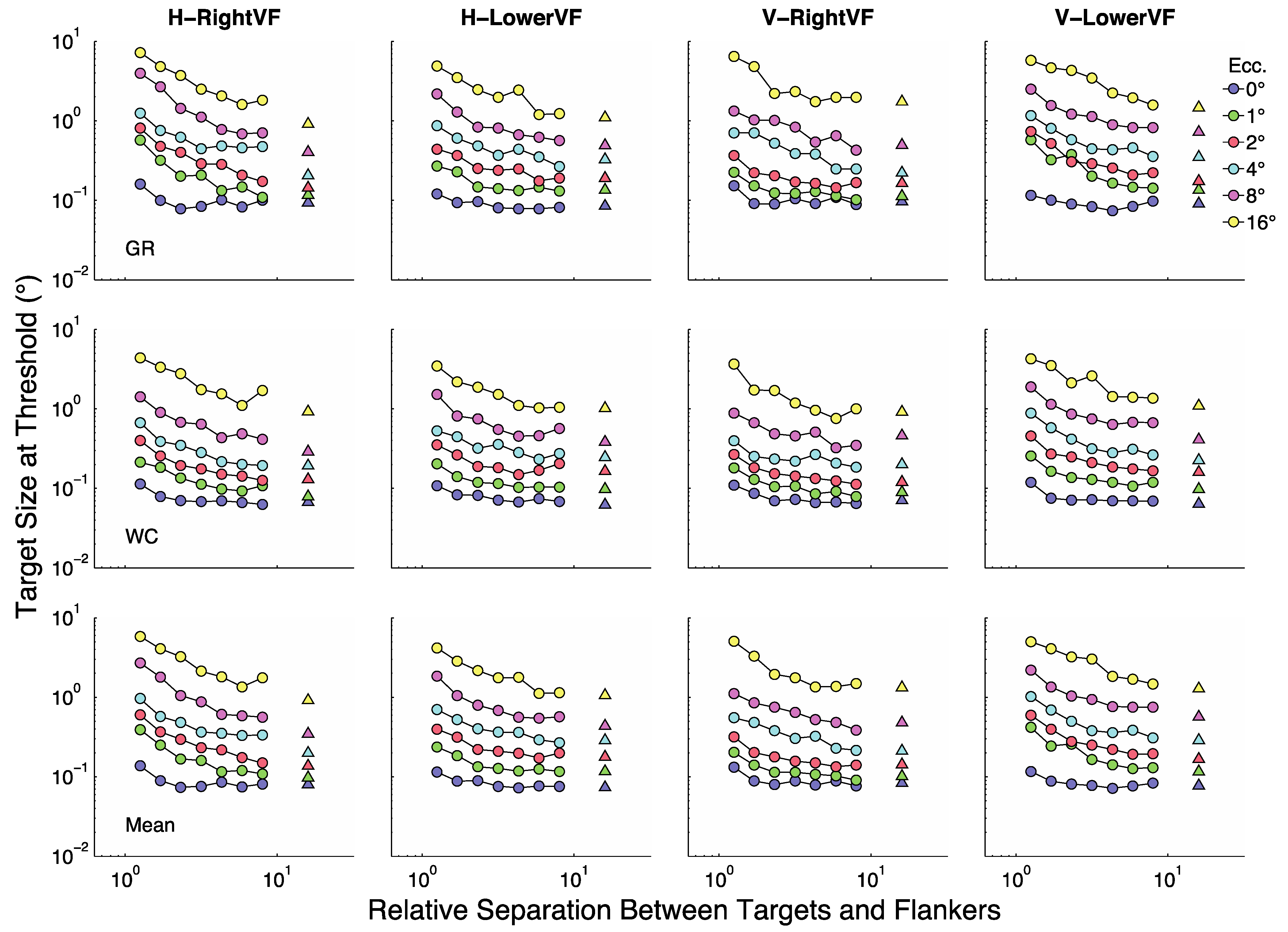
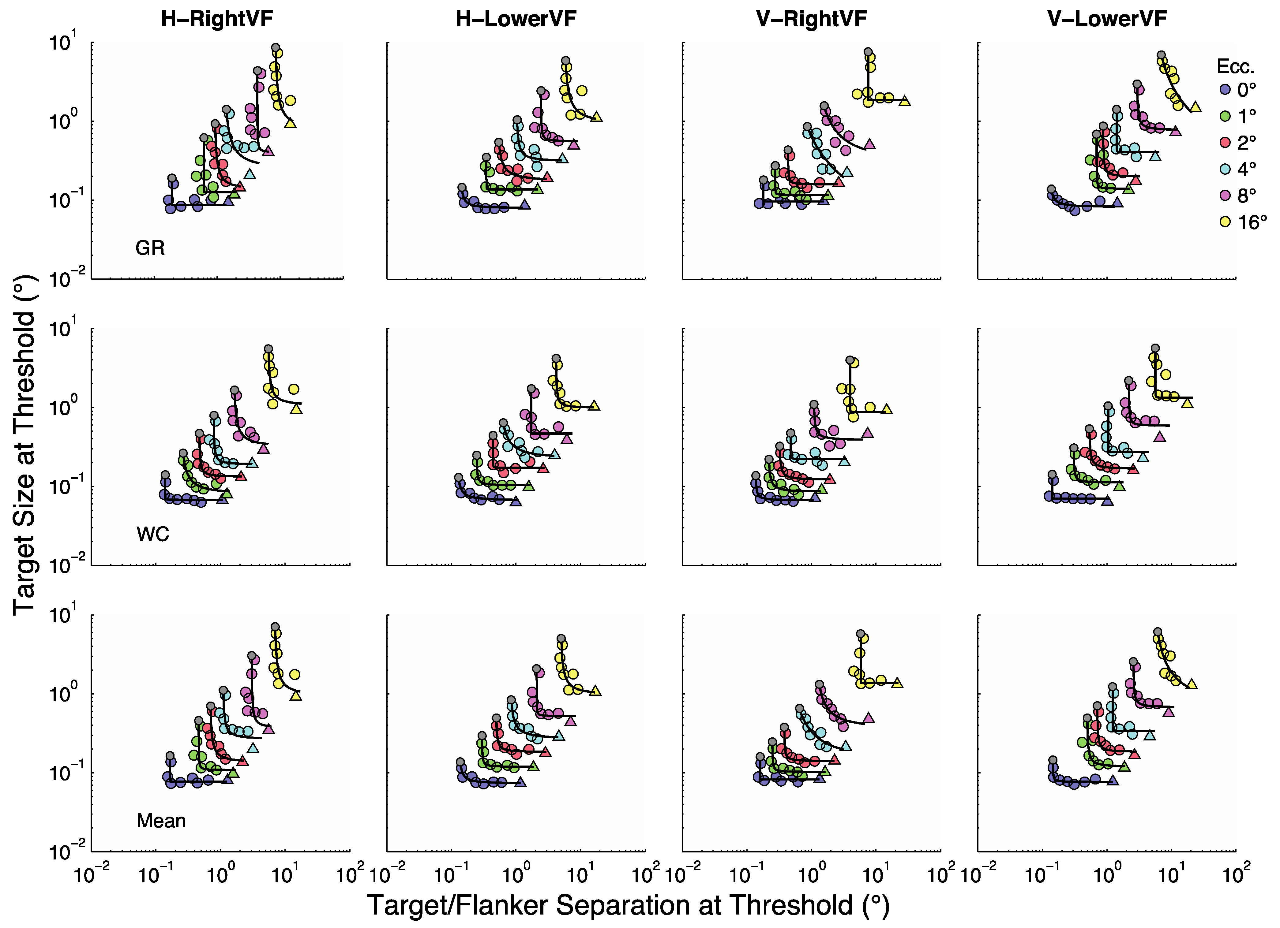
Figure 2 summarizes the results for the two participants (rows 1 and 2) as well as their averaged results (row 3). In each panel the y-axis represents target size (in degrees visual angle) at threshold and the X-axis represents target/flanker separation in multiples of target size (relative separations). Each line (color) represents a given eccentricity as shown in the legend. The four panels in each row show results for the horizontal (H) and vertical (V) flankers when presented in the RightVF or LowerVF. Figure 3 replots the same data with the x-axis as actual separation (in degrees visual angle). Actual separation is obtained by multiplying target size at threshold by the relative separation. The colored circles represent conditions in which the relative separations were 1.25 to 8× target size. Triangles represent the unflanked condition (plotted at 16 times target size in Figure 2 and Figure 3).

Figure 3 shows that at fixation (blue symbols, 0°) size thresholds are largely independent of target-flanker separation for most separations, with modest threshold elevation (increases over the unflanked-condition) at the two smallest separations. At all other eccentricities threshold elevation is considerably greater at the smallest sizes and decreases as separation increases until asymptote is reached at the largest separations. Roughly speaking there are two major parts to most non-foveal curves in Figure 3. At small separations the curves tend to asymptote parallel to the y-axis and at large separations they tend to asymptote parallel to the X-axis. Sections of a curve parallel to the y-axis indicate points at which crowding is independent of target size. That is, the centre-to-centre spacing between targets and flankers does not change with changes in target size. Sections of a curve parallel to the X-axis indicate points at which the flankers have no influence on size thresholds. That is, size thresholds are unchanged as the centre-to-centre spacing between targets and flankers varies.

The general form of the functions in Figure 3 is well captured by a rectangular parabola [31], as defined in Equation 1,

c² = (sep − sep_min)(size − size_min)

(1)

In this case $siz{e}_{min}$ represents the limiting size-at-threshold obtained when target/flanker separation increases towards infinity (i.e., the unflanked condition). In other words, $siz{e}_{min}$ represents the stimulus size at which the curve becomes parallel to the separation axis. And, $se{p}_{min}$ represents the limiting separation-at-threshold obtained when target/flanker separation decreases towards 1 (i.e., the smallest centre-to-centre spacing for which targets and flankers do not overlap). In other words, $se{p}_{min}$ represents the target/flanker separation at which the curve becomes parallel to the size axis. The best fitting rectangular parabola for each curve in Figure 3 is shown as a continuous black line.

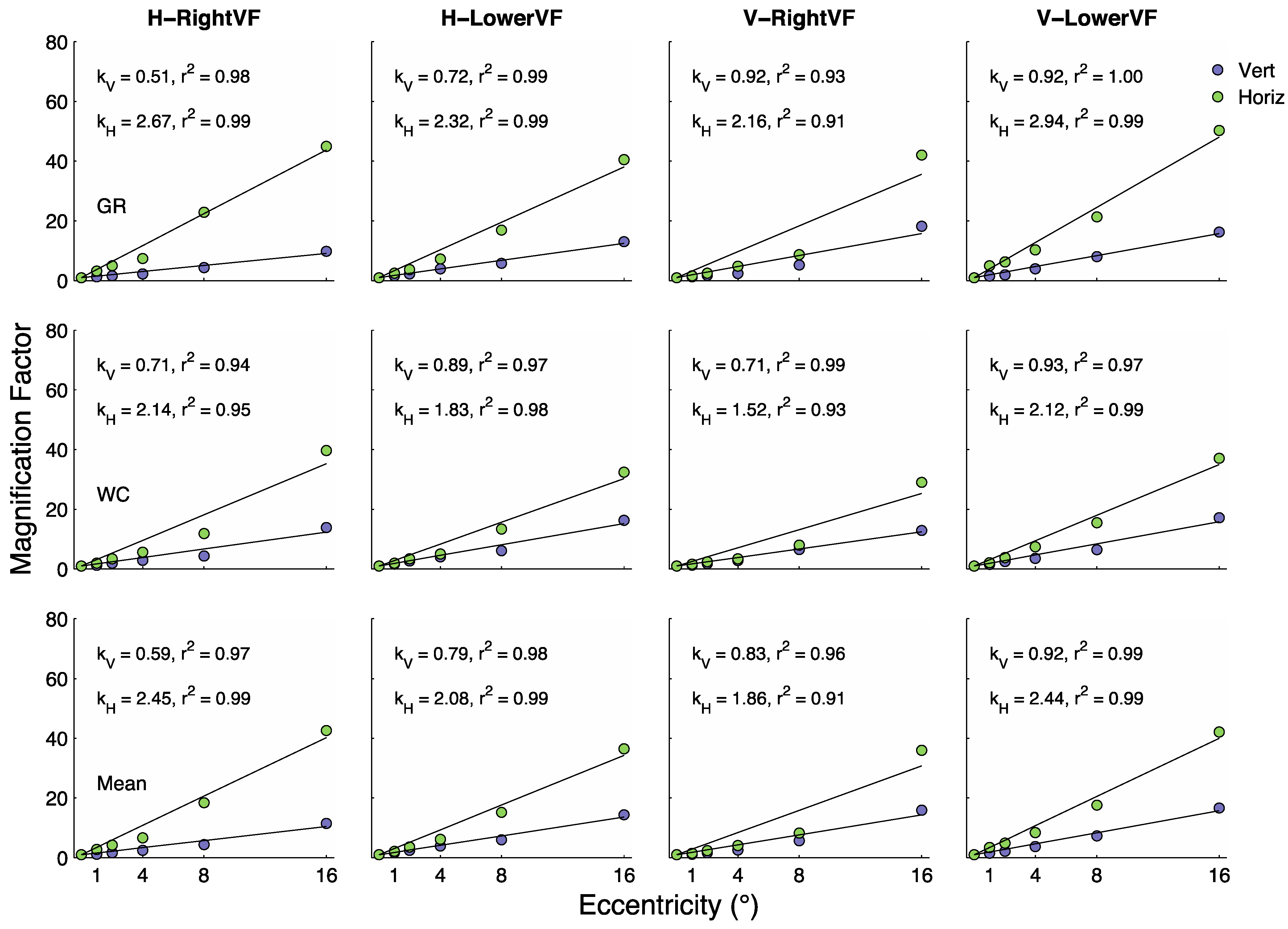
Our objective is to characterize how stimulus size and target/flanker separation combine to determine thresholds across the visual field. A first step in this direction is to consider the limiting cases; i.e., the unflanked thresholds and the smallest possible target/flanker separations. The blue circles in Figure 4 show size thresholds at 1 to 16° relative to size thresholds at fixation; i.e., $s_E/s_0$. The green circles in Figure 4 show the points on the rectangular parabolas at 1 to 16° for which size at threshold (μ_size) = separation at threshold (μ_sep); i.e., μ_size /μ_sep = 1. In other words, the green circles in Figure 4 represent the sizes (or separations) corresponding to the grey dots in Figure 3 at eccentricities of 1 to 16° divided by the sizes (or separations) corresponding to the grey dots at fixation (0°); i.e., μ_E/μ₀. These limiting cases ($s_E/s_0$ and μ_E/μ₀) show how the rectangular parabolas in Figure 3 shift up and to the right with eccentricity, respectively, within each panel.

In each panel of Figure 4 the blue and green data points have been fit with a function of the form $M=1+kE$. The values of $k_V$ and $k_H$ and the proportion of variability ($r^2$) in the data explained by the lines are shown within each panel. In general the fits are quite good, explaining, on average, about 97% of the eccentricity-dependent variability in both $s_E/s_0$ and μ_E/μ₀. The y-axis in Figure 4 is labeled “Magnification Factor” because the curves represent the degree to which the functions shift up and to the right with eccentricity.

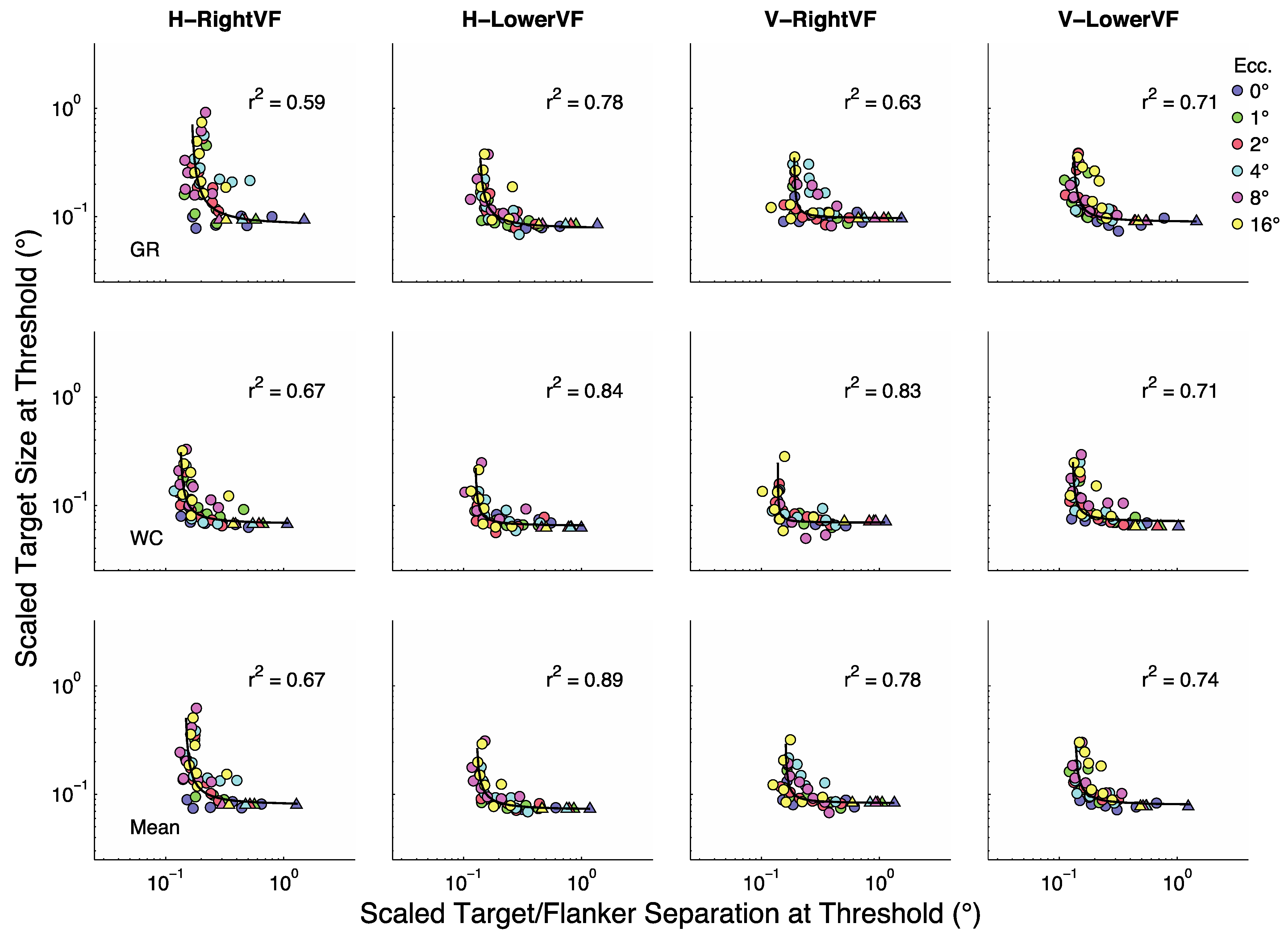
In the large literature on size scaling attempts are made to shift data from all eccentricities onto a single curve in order to provide a concise characterization of the data. For the present data set it is clear that the data would have to be shifted both down and to the left. We used three shifting methods in an attempt to find a simple characterization of the data. First, for each data point in Figure 3 we divided separation at threshold by μ_E/μ₀ and the corresponding size at threshold by $s_E/s_0$. Once the data were shifted downward and leftward in this way, we found the best fitting rectangular parabola to the scaled data. Figure 5 shows the shifted data along with the best-fitting rectangular parabola. Also shown is the proportion of variability that the parabola explains. (Please note that our measure of fit is based on the diagonal distance from data point to curve in the log-log space shown [31]). Generally the fits were reasonably good and explained 72% of the variability in the data on average.

A second analysis was performed to see if a more concise characterization of the data could be achieved by replacing μ_E/μ₀ with $M=1+k_{H}E$ and $s_E/s_0$ with $M=1+k_{V}E$. Once the data were scaled we found the best fitting rectangular parabola. The results are not shown but they explained only 55% of the variability in the data on average, and are therefore substantially worse than the first analysis, which used μ_E/μ₀ and $s_E/s_0$ to scale the data. Therefore, in spite of the seemingly nice fits of $M=1+k_{H}E$ to μ_E/μ₀ and $M=1+k_{V}E$ to $s_E/s_0$ (r² ≈ .97) these approximations leave a great deal of residual variability about the rectangular parabola fit to the scaled data.

A third analysis was performed to see if a better fit could be achieved by replacing linear magnification functions $M=1+k_{H}E$ and $M=1+k_{V}E$ with non-linear magnification functions M = 1+E^αH/β_H and M = 1+E^αV/β_V respectively. We thought these non-linear functions might better fit μ_E/μ₀ and $s_E/s_0$, respectively, and thus produce scaled data that are a better fit to a rectangular parabola. The obtained results explained 63% of the variability in the data and are thus substantially better than the second fit, yet still worse than for the original “raw fits”.

From these analyses we can conclude that the most effective scaling method shifts the curves down and to the left by dividing size at threshold by $s_E/s_0$ and separation at threshold by μ_E/μ₀. It is disappointing that we are unable to find low-parameter fits to these scaling factors that are equally effective. It should be kept in mind, however, that the $r^2$ values reported above do not include variability attributable to eccentricity. That is, the $r^2$ values account only for the variability of the scaled data about the best fitting function. If the fits to the scaled data were “unscaled” by multiplying scaled size at threshold by $s_E/s_0$ and scaled separation at threshold by μ_E/μ₀, the resulting fits to the original data would have produced $r^2$ values that exceed .97, on average, in all cases.

Finally, a number of reports in the crowding literature have shown that crowding is most effective when targets and flankers are aligned with the line that connects them with the point of fixation [23,32]; i.e., horizontally positioned flankers in the RightVF and vertically positioned flankers in the LowerVF. We were able to assess this trend in our data by comparing size at threshold in cases of flankers and targets forming a line connected to fixation to those forming a line perpendicular to this line. In the RightVF this means dividing size thresholds obtained with horizontally oriented flankers by the size thresholds obtained with vertically oriented flankers and in the LowerVF, dividing size thresholds obtained with vertically oriented flankers by the size thresholds obtained with horizontally oriented flankers. These results are shown in Figure 6 for the averaged data. Threshold ratios are shown for each separation and eccentricity in the RightVF and LowerVF. It is notable that in almost all cases the ratios exceed 1, meaning that flankers are more effective when aligned with fixation.

4. Discussion

In this study we asked how flanking items affect the discrimination of symmetry across the visual field. To do this we measured, simultaneously, stimulus size- and target/flanker separation-at threshold across a range of eccentricities in the RightVF and LowerVF. Size thresholds for isolated (unflanked) patches of symmetry (triangles in Figure 3) increased linearly with eccentricity at a relatively modest rate. Figure 4 shows $k_V$ values ranging from 0.51 to 0.93, with a mean of ${\overline{k}}_V$ = .79 (SEM = .053). These results are generally consistent with several previous studies that asked the same question with somewhat different methods [12,14,15,16]. A report by Barrett et al. [14] found average values of $k_V$ = 1.21, but within this average one subject had $k_V$ = 0.97 and the other had $k_V$ = 1.62. A study by Saarinen [15] found that $k_V$ = 1.29 accounted for the data and a study by Sally and Gurnsey [16] found that $k_V$ = 0.88 averaged over conditions and subjects; the range was 0.49 to 1.14. As noted, some of this variability may be attributable to subject differences. However, some of this variability may be attributable to the nature of symmetry itself. In most studies of symmetry, symmetrical patches are generated randomly on each trial. Therefore, subjects cannot perform the task through a template-matching strategy. The downside of this stochastic stimulus generation is that two nominally identical stimuli (e.g., stimuli of identical size) might actually differ in “perceptual salience”. This inherent variability makes it difficult to estimate thresholds reliably. In fact, the data reported in Figure 3, for example, are more variable than comparable data we have obtained [25] in similar tasks (letter identification, and grating [≡ ⫴] and “T” [⊤ ⊢ ⊥ ⊣] orientation discrimination) that do not have this stochastic characteristic.

Changes with eccentricity in μ_size (or μ_sep) for which μ_size/μ_sep = 1, reflect the changes in the maximum crowding effects with eccentricity; i.e., greatest extent of the crowding region or greatest elevation of target size at threshold. Figure 4 (green circles) shows that the magnitude of crowding increases with eccentricity at a faster rate than changes in size thresholds in the unflanked conditions. Using the best-fitting linear fits to these data gives a mean ${\overline{k}}_H$ = 2.21 (SEM = 0.16), which is about 2.8 times greater than ${\overline{k}}_V$ = 0.79. Therefore, in the case of symmetry discrimination we find that crowding effects increase with eccentricity at a greater rate than unflanked size-thresholds, as found in several previous studies employing different stimuli and tasks [22,23,25]. Clearly, symmetry is not exempt from crowding effects.

We noted earlier that the evidence shows clearly that bilateral symmetry does not pop-out of complex displays [10,11]. In addition, evidence suggests that symmetry does not provide an alerting signal when surrounded by non-symmetrical noise [12] in peripheral vision. The present study extends what is known about sensitivity to symmetry in the visual periphery by showing that symmetry is susceptible to interference from flanking items in peripheral vision. We have recently employed the methodology used here to examine crowding effects for letter identification, and grating and “T” orientation discrimination tasks. In all these cases the growth of interference regions with eccentricity (the horizontal shifts of the curves in Figure 3; green symbols in Figure 4) is much faster than the loss of resolution with eccentricity (the vertical shifts of the curves in Figure 3; blue symbols in Figure 4). However, tasks differ with respect to the relative rates at which the extent of interference zones and resolution limits change with eccentricity. For example, the horizontal magnification factor (μ_E/μ₀) for grating and T orientation discrimination tasks reach levels of 54 and 58, respectively at 16° in the LowerVF, whereas for letter discrimination this ratio reaches only 33 at 16°. In the present tasks, averaged over observers and conditions we find that the μ_E/μ₀ reaches 38 at 16°. Interestingly, we found ${\overline{k}}_V$ = 0.79 in the present symmetry task, 0.759 in the letter discrimination task and 0.54 and 0.57 in the grating and T orientation tasks. Therefore, in terms of these metrics the symmetry tasks studied here have more in common with the letter identification task than the grating and T orientation discrimination tasks.

The similarity of the symmetry results and the letter task (and their difference from the grating and T orientation tasks) may have something to do with the complexity of the decision to be made. We might have expected the symmetry tasks to have more in common with the grating and T orientation tasks, than the letter identification task. After all, we asked subjects to judge the orientation of the axis of symmetry. On the other hand, the perceptual complexity of the symmetrical stimuli may be more akin to the perceptual complexity of the letters. It may be that orientation discrimination for simple figures is a relatively simple task and hence the relatively slower rates of eccentricity-dependent sensitivity loss whereas the more demanding tasks (letter and symmetry discrimination) produce faster rates of eccentricity dependent sensitivity loss.

We found little evidence of crowding at fixation, however, there was some evidence of crowding at the smallest two relative separations (1.25, 1.70), consistent with previous findings that suggest the extent of spatial interaction extends over a very small range [22,24,32]. The smallest relative separation (1.25) translates to a centre-to-centre spacing of 0.15° on average at fixation. As the crowding effect at fovea is modest at best and only for the two smallest distances between target and flanker it could be the result of internal blur given the complexity of our stimulus pattern [24]. A consistent issue in the crowding literature is the near impossibility of making the stimuli at fixation (e.g., target and flankers) smaller than the internal blur while still being able to measure performance. As a result crowding and masking may get confused in the fovea because of the effects of blur, so that what looks like crowding is actually partly masking [33].

Finally, Figure 6 shows that in both cases target to fixation size thresholds are higher when the flankers are aligned (parallel) with the axis. This is in keeping with literature that suggests that crowding zones are elliptical and oriented to the fovea [23,34].

5. Conclusions

The present paper demonstrates that there are two eccentricity-dependent limits on symmetry perception. The first is a simple loss of resolution with eccentricity, and this can be compensated for by stimulus magnification. The second involves susceptibility to interference by flanking items. The extent of this interference increases with eccentricity, and generally this rate is faster than the rate of resolution loss. It is also the case, as with other instances of crowding, that interference is greatest when the targets and flankers form a line that connects the centre of the target to the point of fixation. We found very little evidence of crowding at fixation, consistent with recent work in our lab [25] and several other labs [23,34]. The similarity of the present results, using symmetrical targets, and previous results using letter like stimuli, suggest that symmetry is not particularly special to the early visual system, even though it is clearly important at a conceptual and aesthetic level.

References

- Møller, A. Female swallow preference for symmetrical male sexual ornaments. Nature 1992, 357, 238–240. [Google Scholar] [CrossRef]
- Swaddle, J.; Cuthill, I. Preference for symmetric males by female zebra finches. Nature 1994, 367, 165–166. [Google Scholar] [CrossRef]
- Horridge, G. The honeybee (apis mellifera) detects bilateral symmetry and discriminates its axis. J. Insect Physiol. 1996, 42, 755–764. [Google Scholar] [CrossRef]
- van der Helm, P. The influence of perception on the distribution of multiple symmetries in nature and art. Symmetry 2011, 3, 54–71. [Google Scholar] [CrossRef]
- Wagemans, J. Skewed symmetry: A nonaccidental property used to perceive visual forms. J. Exp. Psychol. Hum. Percept. Perform. 1993, 19, 364–380. [Google Scholar] [CrossRef] [PubMed]
- Wagemans, J. Detection of visual symmetries. Spat. Vis. 1995, 9, 9–32. [Google Scholar] [CrossRef]
- Barlow, H.B.; Reeves, B.C. The versatility and absolute efficiency of detecting mirror symmetry in random dot displays. Vis. Res. 1979, 19, 783–793. [Google Scholar] [CrossRef]
- van der Helm, P.A.; Leeuwenberg, E.L. Goodness of visual regularities: a nontransformational approach. Psychol. Rev. 1996, 103, 429–456. [Google Scholar] [CrossRef]
- Treisman, A.M.; Gelade, G. A feature-integration theory of attention. Cognit. Psychol. 1980, 12, 97–136. [Google Scholar] [CrossRef]
- Gurnsey, R.; Herbert, A.; Nguyen-Tri, D. Bilateral Symmetry is not detected in parallel. In Proceedings of the Annual Meeting of the Canadian Society for Brain, Behaviour and Cognitive Science, Ottawa, ON, Canada, 18–21 June 1998. [Google Scholar]
- Olivers, C.N.; van der Helm, P.A. Symmetry and selective attention: A dissociation between effortless perception and serial search. Percept. Psychophys. 1998, 60, 1101–1116. [Google Scholar] [CrossRef]
- Gurnsey, R.; Herbert, A.M.; Kenemy, J. Bilateral symmetry embedded in noise is detected accurately only at fixation. Vis. Res. 1998, 38, 3795–3803. [Google Scholar] [CrossRef]
- Weymouth, F.W. Visual sensory units and the minimal angle of resolution. Am. J. Ophthalmol. 1958, 46, 102–113. [Google Scholar] [CrossRef]
- Barrett, B.T.; Whitaker, D.; McGraw, P.V.; Herbert, A.M. Discriminating mirror symmetry in foveal and extra-foveal vision. Vis. Res. 1999, 39, 3737–3744. [Google Scholar] [CrossRef]
- Saarinen, J. Detection of mirror symmetry in random dot patterns at different eccentricities. Vis. Res. 1988, 28, 755–759. [Google Scholar] [CrossRef]
- Sally, S.L.; Gurnsey, R. Symmetry detection across the visual field. Spat. Vis. 2001, 14, 217–234. [Google Scholar] [PubMed]
- Tyler, C.W. Human symmetry detection exhibits reverse eccentricity scaling. Vis. Neurosci. 1999, 16, 919–922. [Google Scholar] [CrossRef] [PubMed]
- Gurnsey, R.; Poirier, F.J.; Bluett, P.; Leibov, L. Identification of 3D shape from texture and motion across the visual field. J. Vis. 2006, 6, 543–553. [Google Scholar] [CrossRef]
- Gurnsey, R.; Roddy, G.; Ouhnana, M.; Troje, N.F. Stimulus magnification equates identification and discrimination of biological motion across the visual field. Vis. Res. 2008, 48, 2827–2834. [Google Scholar] [CrossRef]
- Gurnsey, R.; Roddy, G.; Troje, N.F. Limits of peripheral direction discrimination of point-light walkers. J. Vis. 2010, 10, 1–17. [Google Scholar] [CrossRef]
- Whitaker, D.; Rovamo, J.; MacVeigh, D.; Mäkelä, P. Spatial scaling of vernier acuity tasks. Vis. Res. 1992, 32, 1481–1491. [Google Scholar] [CrossRef]
- Latham, K.; Whitaker, D. Relative roles of resolution and spatial interference in foveal and peripheral vision. Ophthalmic Physiol. Opt. 1996, 16, 49–57. [Google Scholar] [CrossRef]
- Toet, A.; Levi, D.M. The two-dimensional shape of spatial interaction zones in the parafovea. Vis. Res 1992, 32, 1349–1357. [Google Scholar] [CrossRef]
- Levi, D.M. Crowding--an essential bottleneck for object recognition: A mini-review. Vis. Res. 2008, 48, 635–654. [Google Scholar] [CrossRef] [PubMed]
- Gurnsey, R.; Roddy, G.; Chanab, W. Crowding is eccentricity and size dependent. J. Vis. 2011, 11. [Google Scholar] [CrossRef]
- Kennedy, G.J.; Whitaker, D. The chromatic selectivity of visual crowding. J. Vis. 2010, 10, 15. [Google Scholar] [CrossRef]
- Levi, D.M.; Carney, T. Crowding in peripheral vision: why bigger is better. Curr. Biol. 2009, 19, 1988–1993. [Google Scholar] [CrossRef]
- Bach, M. The Freiburg Visual Acuity test--automatic measurement of visual acuity. Optom. Vis. Sci. 1996, 73, 49–53. [Google Scholar] [CrossRef] [PubMed]
- Kleiner, M.; Brainard, D.H.; Pelli, D.G. What’s new in Psychtoolbox-3? Eur. Conf. Visual Percept. 2007, 36, 1–14. [Google Scholar]
- Watson, A.B.; Pelli, D.G. QUEST: A Bayesian adaptive psychometric method. Percept. Psychophys. 1983, 33, 113–120. [Google Scholar] [CrossRef]
- Poirier, F.J.; Gurnsey, R. Two eccentricity-dependent limitations on subjective contour discrimination. Vis. Res. 2002, 42, 227–238. [Google Scholar] [CrossRef]
- Pelli, D.G.; Tillman, K.A.; Freeman, J.; Su, M.; Berger, T.D.; Majaj, N.J. Crowding and eccentricity determine reading rate. J. Vis. 2007, 7, 21–36. [Google Scholar] [CrossRef] [PubMed]
- Levi, D.M.; Klein, S.A.; Hariharan, S. Suppressive and facilitatory spatial interactions in foveal vision: foveal crowding is simple contrast masking. J. Vis. 2002, 2, 140–166. [Google Scholar] [CrossRef] [PubMed]
- Pelli, D.G.; Palomares, M.; Majaj, N.J. Crowding is unlike ordinary masking: distinguishing feature integration from detection. J. Vis. 2004, 4, 1136–1169. [Google Scholar] [CrossRef] [PubMed]
Figure 1.
Trigrams used for Experiment 1. The central element (target) was a symmetrical patch that could have a vertical (shown) or horizontal (not shown) axis of symmetry. The flankers could be above and below or to the left and right of the target. The entire configuration (trigram) could be parallel to or perpendicular to the line that connects the central target to the point of fixation. Note, the target and flankers were presented on a uniform grey background.
Figure 2.
Size at threshold as a function of relative target/flanker separation at each eccentricity. Rows 1 and 2 plot results for two subjects and row 3 plots mean results. The four columns represent the four combinations of flanker positions with respect to the target (H and V) and position in the visual field (RightVF and LowerVF). Symbol colors represent eccentricities of 0 to 16°, as shown in the legend. Circles represent target/flanker separations of 1.25 to 8 times target size at each eccentricity. Triangles represent the unflanked condition at each eccentricity; these are depicted at 16 times target size for illustration.
Figure 3.
Size at threshold as a function of the target/flanker separation at threshold. (Target/flanker separation at threshold = target size at threshold * relative separation.) Rows 1 and 2 plot results for two subjects and row 3 plots mean results. The four columns represent the four combinations of flanker positions with respect to the target (H and V) and position in the visual field (RightVF and LowerVF). Circles represent target/flanker separations of 1.25 to 8 times target size at each eccentricity. Triangles represent the unflanked condition at each eccentricity; these are depicted at 16 times target size for illustration. The continuous curves show the best fitting rectangular parabola; see text for details. The small gray point at the upper end of each curve represents the point on the curve for which size at threshold equals separation at threshold.
Figure 4.
Horizontal and vertical magnification factors. The x-axes represent eccentricity in degrees visual angle. The blue circles represent target size at threshold in the unflanked conditions divided by target size at threshold at fixation (0°). These ratios show how the curves in Figure 3 shift upwards with eccentricity. The green circles represent sizes (and separations) for which size = separation at threshold divided by the same quantity obtained at fixation. These ratios show how the curves in Figure 3 shift rightwards with eccentricity. and are linear approximations to these vertical and horizontal shifts. In each panel and that best fit the data are shown along with the proportion of variability () they explain in the data.
Figure 5.
Scaled target size at threshold vs. scaled target/flanker separation at threshold. (See text for details.) The four columns represent the four combinations of flanker positions with respect to the target (H and V) and position in the visual field (RightVF and LowerVF). Symbol colors represent eccentricities of 0 to 16°. Circles represent target/flanker separations of 1.25 to 8 times target size at each eccentricity. Triangles represent the unflanked condition at each eccentricity; these are depicted at 16 times target size.
Figure 6.
Effect target/flanker configuration in the RightVF and LowerVF. The ratio of size threshold for parallel flankers to perpendicular flankers is shown as a function of relative separation for the RightVF and LowerVF. The ratios have been formed from the average data (row three) from Figure 2.
© 2011 by the authors; licensee MDPI, Basel, Switzerland. This article is an open access article distributed under the terms and conditions of the Creative Commons Attribution license (http://creativecommons.org/licenses/by/3.0/).
Share and Cite
MDPI and ACS Style
Roddy, G.; Gurnsey, R. Mirror Symmetry Is Subject to Crowding. Symmetry 2011, 3, 457-471. https://doi.org/10.3390/sym3030457
AMA Style
Roddy G, Gurnsey R. Mirror Symmetry Is Subject to Crowding. Symmetry. 2011; 3(3):457-471. https://doi.org/10.3390/sym3030457
Chicago/Turabian StyleRoddy, Gabrielle, and Rick Gurnsey. 2011. "Mirror Symmetry Is Subject to Crowding" Symmetry 3, no. 3: 457-471. https://doi.org/10.3390/sym3030457