Intrinsic Symmetry Groups of Links with 8 and Fewer Crossings

Abstract

We present an elementary derivation of the “intrinsic” symmetry groups for links of 8 or fewer crossings. We show that standard invariants are enough to rule out all potential symmetries outside the symmetry group of the group of the link for all but one of these links and present explicit isotopies generating the symmetry group for every link.

1. Introduction

The symmetry group of a link L is defined to be the mapping class group $MCG\left(L\right)$ (or $Sym\left(L\right)$) of the pair $(S^3,L)$. The study of this symmetry group is a classical topic in knot theory, and these groups have now been computed for prime knots and links in several ways. Kodama and Sakuma [1] used a method in Bonahon and Siebenmann [2] to compute these groups for all but three of the knots of 10 and fewer crossings in 1992. In the same year, Weeks and Henry used the program SnapPea to compute the symmetry groups for hyperbolic knots and links of 9 and fewer crossings [3]. These efforts followed earlier tabulations of symmetry groups by Boileau and Zimmermann [4], who found symmetry groups for non-elliptic Montesinos links with 11 or fewer crossings.

We consider a different group of symmetries of a link L given by the image of the natural homomorphism

$$\pi :Sym\left(L\right)=MCG(S^3,L)\to MCG\left(S^3\right)\times MCG\left(L\right)$$

Since these symmetries record an action on L itself (and only record the orientation of the ambient $S^3$), we will call them “intrinsic” symmetries of L to distinguish them from the standard symmetry group and denote them as $\Sigma \left(L\right)$, cf. Definition 4.5. Following Whitten [5], we denote all possible intrinsic symmetries as $\Gamma \left(L\right)=MCG\left(S^3\right)\times MCG\left(L\right)$; see Definition 4.1.

Unlike the elements in the Sym group, which may be somewhat difficult to describe explicitly, each of the elements in $\Sigma \left(L\right)$ corresponds to an isotopy of L which may exchange the position of some components, which may reverse the orientation of the ambient space—this mirrors any diagram of L, and which may reverse orientations of some components. Neither the Boileau–Zimmerman or the Henry–Weeks-SnapPea method gives much insight into what those isotopies might look like. In addition, it is worth noting that SnapPea is a large and complicated computer program, and while its results are accurate for the links in our table, it is always worthwhile to have alternate proofs for results that depend essentially on nontrivial computer calculations.

In this spirit, the present paper presents an elementary and explicit derivation of the $\Sigma \left(L\right)$ groups for all links of 8 and fewer crossings. We rule out certain isotopies using elementary and polynomial invariants to provide an upper bound on the size of $\Sigma \left(L\right)$ for each link in our table and then present explicit isotopies generating $\Sigma \left(L\right)$ starting with the configurations of the link in Cerf’s table of alternating oriented links [6] or (for nonalternating links) Doll and Hoste’s table [7]. For two links in our table, $7_6^2$ and $8_{13}^2$, an additional construction is needed to rule out certain “component exchange” symmetries using satellites and the Jones polynomial. This shows that the polynomial invariants are powerful enough to compute $\Sigma \left(L\right)$ for these links. For one link in our table, $8_5^3$, even this construction does not rule out all the isotopies outside the symmetry group and we must fall back on the hyperbolic structure of the link to compute the symmetry group. We give the first comprehensive list of $\Sigma \left(L\right)$ groups that we know of, though Hillman [8] provides examples of various two-component links (including some split links) with symmetry groups equal to 12 different subgroups of ${\Gamma }_2$.

Why are the $\Sigma \left(L\right)$ groups interesting? First, it is often more natural to consider the restricted group $\Sigma \left(L\right)$ than the generally larger $Sym\left(L\right)$. Sakuma [9] has shown that a knot K has a finite symmetry group if and only if K is a hyperbolic knot, a torus knot, or a cable of a torus knot. Thus for many [10] knots, the group $Sym\left(L\right)$ contains infinitely many elements which act nontrivially on the complement of L but fix the link itself. We ignore such elements, which lie in the kernel of the natural homomorphism $\pi :MCG(S^3,L)\to MCG\left(S^3\right)\times MCG\left(L\right)$. In fact, even when $MCG(S^3,L)$ is finite, we give various examples below where $\pi$ has nontrivial kernel. It is often difficult to describe an element of $Sym\left(L\right)$ in $ker\pi$ explicitly, but it is always simple to understand the exact meaning of the statement $\gamma \in \Sigma \left(L\right)$.

As an application, if one is interested in classifying knots and links up to oriented, labeled ambient isotopy, it is important to know the symmetry group $\Sigma \left(L\right)$ for each prime link type L, since links related by an element in $\Gamma \left(L\right)$ outside $\Sigma \left(L\right)$ are not (oriented, labeled) ambient isotopic. The number of different links related by an element of $\Gamma \left(L\right)$ to a given link of prime link type L is given by the number of cosets of $\Sigma \left(L\right)$ in $\Gamma \left(L\right)$. If we count these cosets instead of prime link types, the number of actual knots and link types of a given crossing number is actually quite a bit larger than the usual table of prime knot and link types suggests. (See

Table 1. This table shows the number of distinct isotopy classes of links by crossing number and number of components in the link. The columns labeled “n-U” count link types for n-component links in the usual way, where the components are unlabeled and unoriented, and the mirror image of a given link is considered to have the same link type, regardless of whether the two are ambient isotopic. The columns labeled “n-OS” give finer information, considering two n-component links to have the same type if and only if they are oriented, labeled ambient isotopic. As we can see, this stricter definition leads to a much larger collection of link types.

Crossings	Number of link types by components and crossings
	1-U	1-OS	2-U	2-OS	3-U	3-OS	4-U	4-OS	All Links-U	All Links-OS
2			1	2					1	2
3	1	2
4	1	1	1	4					1	4
5	2	4	1	2					1	2
6	3	5	3	10	3	18			6	44
7	7	14	8	38	1	8			9	40
8	21	38	16	78	10	200	3	120	29	398

.)

Second, $\Sigma \left(L\right)$ seems likely to be eventually relevant in applications. For instance, when studying DNA links, each loop of the link generally has a unique sequence of base pairs which provide an orientation and an unambiguous labeling of each component of the link. In such a case, the question of whether two components in a link can be interchanged may prove to be of real significance.

Last, we are interested in the topic of tabulating composite knots and links. Since the connect sum of different symmetry versions of the same knot type can produce different knots (such as the square knot, which is the connect sum of a trefoil and its mirror image, and the granny knot, which is the connect sum of two trefoils with the same handedness), keeping track of the action of $\Sigma \left(L\right)$ is a crucial element in this calculation. We treat this topic in a forthcoming manuscript [11].

2. The Symmetry and Intrinsic Symmetry Groups

As we will describe below, the group $MCG\left(S^3\right)\times MCG\left(L\right)$ was first studied by Whitten in 1969 [5], following ideas of Fox. They denoted this group $\Gamma \left(L\right)$ or ${\Gamma }_{\mu }$, where $\mu$ is the number of components of L. We can write this group as a semidirect product of ${\mathbf{Z}}_2$ groups encoding the orientation of each component of the link L with the permutation group $S_{\mu }$ exchanging components of L (cf. Definition 4.1), finally crossed with another ${\mathbf{Z}}_2$ recording the orientation of $S^3$:

$$\Gamma \left(L\right)={\Gamma }_{\mu }={\mathbf{Z}}_2\times ({\mathbf{Z}}_2^{\mu }⋊S_{\mu })$$

It is clear that an element $\gamma =({ϵ}_0,{ϵ}_1,\dots ,{ϵ}_{\mu },p)\in \Gamma \left(L\right)$ acts on L to produce a new link $L^{\gamma }$. If ${ϵ}_0=+1$, then $L^{\gamma }$ and L are the same as sets (but the components of L have been renumbered and reoriented), while if ${ϵ}_0=-1$ the new link $L^{\gamma }$ is the mirror image of L (again with renumbering and reorientation). We can then define the symmetry subgroup $\Sigma \left(L\right)$ by

$$\gamma \in \Sigma \left(L\right)\iff \mathrm{there}\mathrm{is}\mathrm{an}\mathrm{isotopy}\mathrm{from}L\mathrm{to}{L}^{\gamma }\mathrm{preserving}\mathrm{component}\mathrm{numbering}\mathrm{and}\mathrm{orientation}.$$

For knots, $\Sigma \left(L\right)<{\Gamma }_1={\mathbf{Z}}_2\times {\mathbf{Z}}_2$. Here the five subgroups of ${\mathbf{Z}}_2\times {\mathbf{Z}}_2$ correspond to the standard descriptions of the possible symmetries for a knot, as shown in

Table 2. The five standard symmetry types for knots correspond to the five subgroups of the Whitten group ${\Gamma }_1$.

Symmetry subgroup of ${\mathbf{\Gamma }}_1$	Name	Example(s)
$\left\{\right(1,1\left)\right\}$	No symmetry	$9_{32},9_{33}$
$\left\{\right(1,1),(-1,1\left)\right\}$	(+) amphichiral symmetry	${12}_{427}$
$\left\{\right(1,1),(1,-1\left)\right\}$	invertible 1 symmetry	$3_1$
$\left\{\right(1,1),(-1,-1\left)\right\}$	(−) amphichiral 2 symmetry	$8_{17}$
${\Gamma }_1$	full symmetry	$4_1$

¹ Conway [12] calls this reversible symmetry; ² Conway [12] calls this invertible symmetry.

.

For links, the situation is more interesting, as the group $\Gamma \left(L\right)$ is more complicated. In the case of two-component links, the group ${\Gamma }_2={\mathbf{Z}}_2\times ({\mathbf{Z}}_2\times {\mathbf{Z}}_2⋊S_2)$ is a non-Abelian 16 element group isomorphic to ${\mathbf{Z}}_2\times D_4$. The various subgroups of ${\Gamma }_2$ do not all have standard names, but we will call a link purely invertible if $(1,-1,\dots ,-1,e)\in \Sigma \left(L\right)$, and say that components $(i,j)$ have a pure exchange symmetry if $(1,1,\dots ,1,(ij\left)\right)\in \Sigma \left(L\right)$. For two-component links, we will say that L has pure exchange symmetry if its two components have that symmetry. The question of which links have this symmetry goes back at least to Fox’s 1962 problem list in knot theory, cf. Problem 11 in [13] and [14]. For example, $2_1^2$ (the Hopf link) has pure exchange symmetry while we will show that $7_4^2$ does not.

We similarly focus on the pure invertibility symmetry: we show that 45 out of the 47 prime links with 8 crossings or less are purely invertible. The two exceptions are $6_2^3$ (the Borromean rings) and $8_5^3$; we show that both of these are invertible using some nontrivial permutation, i.e., $(1,-1,-1,-1,p)\in \Sigma \left(L\right)$ for some $p\ne e$. (Whitten found examples of more complicated links which are not invertible even when a nontrivial permutation is allowed [15].)

Increasing the number of components in a link greatly increases the number of possible types of symmetry.

Table 3. The number of subgroups of ${\Gamma }_{\mu }$; each one represents a different intrinsic symmetry group possible for a $\mu$-component link. The number of nonconjugate symmetries (the fourth column) is given by the number of conjugacy classes of subgroups. This article computes the symmetry group for all prime links of 8 or fewer crossings; the last column summarizes our results.

$\mathit{\mu }$	$\left|{\mathbf{\Gamma }}_{\mathit{\mu }}\right|$	# subgroups	# subgroups	nonconjugate ones
			(up to conjugacy)	for $\le 8$ crossings
1	4	5	5	3
2	16	35	27	5
3	96	420	131	7
4	768	9,417	994	3
5	7,680	270,131	6,382	0

lists the number of subgroups of ${\Gamma }_{\mu }$; each different subgroup represents a different intrinsic symmetry group that a $\mu$-component link might have. We note that if $\Sigma \left(L\right)$ is the symmetry subgroup of link L, then the symmetry subgroup of $L^{\gamma }$ is the conjugate subgroup $\Sigma \left(L^{\gamma }\right)=\gamma \Sigma \left(L\right){\gamma }^{-1}$. Therefore, it suffices to only examine the number of mutually nonconjugate subgroups of ${\Gamma }_{\mu }$ in order to specify all of the different intrinsic symmetry groups. Table 3 also lists the number of conjugacy classes of subgroups of ${\Gamma }_{\mu }$, and the number of these which appear for prime links of 8 or fewer crossings.

3. Methods and Notation

We started from the excellent table of oriented alternating links provided by Cerf [6]. Cerf considers the effect of reversing orientations of components of her links, but does not compute the effect of permutations. Our more detailed calculation does not depend on this information, so our paper also provides a check on Cerf’s symmetry calculations. For alternating links, we have kept component numbers and orientations consistent with her table. For non-alternating links, we use component numbers and orientations consistent with those of Doll and Hoste [7]. Like Cerf, Doll and Hoste considered the effect of reversing the orientation of individual components of these links, but not the effect of permutations of components. We note that these component numbers and orientations are not consistent with those used in SnapPea. The component numbers and orientations in SnapPea seem to have been chosen arbitrarily sometime in the $1980s$ by Joe Christy when he digitized the Rolfsen table [16].

To check our results against the SnapPea calculations, we used the Python interface provided by SnapPy [17] to compute the image of $\pi :MCG(S^3,L)\to MCG\left(S^3\right)\times MCG\left(L\right)$. The results agreed [18] with the tables we give below, meaning that our results serve as an independent verification of SnapPea’s accuracy for all of these links except $8_5^3$ (which uses SnapPea to rule out a single potential symmetry).

Finally, some notational comments: we henceforth use the term ‘link’ to refer to a prime, multicomponent link unless otherwise indicated. We use the Rolfsen notation for links but provide the Thistlethwaite notation as well in our summary tables (

Table 4. The Whitten symmetry group for each two-component link.

Link	$\Sigma$ Group	Link	$\Sigma$ Group	Link	$\Sigma$ Group
$2_1^2\left(2a1\right)$	${\Sigma }_{8,2}$	$7_5^2\left(7a2\right)$	${\Sigma }_{2,1}$	$8_7^2\left(8a8\right)$	${\Sigma }_{4,1}$
$4_1^2\left(4a1\right)$	${\Sigma }_{4,1}$	$7_6^2\left(7a1\right)$	${\Sigma }_{4,2}$	$8_8^2\left(8a9\right)$	${\Sigma }_{8,2}$
$5_1^2\left(5a1\right)$	${\Sigma }_{8,1}$	$7_7^2\left(7n1\right)$	${\Sigma }_{2,1}$	$8_9^2\left(8a3\right)$	${\Sigma }_{2,1}$
$6_1^2\left(6a3\right)$	${\Sigma }_{4,1}$	$7_8^2\left(7n2\right)$	${\Sigma }_{4,2}$	$8_{10}^2\left(8a2\right)$	${\Sigma }_{4,2}$
$6_2^2\left(6a2\right)$	${\Sigma }_{8,2}$	$8_1^2\left(8a14\right)$	${\Sigma }_{4,1}$	$8_{11}^2\left(8a5\right)$	${\Sigma }_{2,1}$
$6_3^2\left(6a1\right)$	${\Sigma }_{4,1}$	$8_2^2\left(8a12\right)$	${\Sigma }_{4,1}$	$8_{12}^2\left(8a4\right)$	${\Sigma }_{4,2}$
$7_1^2\left(7a6\right)$	${\Sigma }_{4,1}$	$8_3^2\left(8a11\right)$	${\Sigma }_{4,1}$	$8_{13}^2\left(8a1\right)$	${\Sigma }_{4,2}$
$7_2^2\left(7a5\right)$	${\Sigma }_{4,1}$	$8_4^2\left(8a13\right)$	${\Sigma }_{4,1}$	$8_{14}^2\left(8a7\right)$	${\Sigma }_{2,1}$
$7_3^2\left(7a4\right)$	${\Sigma }_{8,1}$	$8_5^2\left(8a10\right)$	${\Sigma }_{4,1}$	$8_{15}^2\left(8n2\right)$	${\Sigma }_{4,2}$
$7_4^2\left(7a3\right)$	${\Sigma }_{4,2}$	$8_6^2\left(8a6\right)$	${\Sigma }_{4,1}$	$8_{16}^2\left(8n1\right)$	${\Sigma }_{2,1}$

,

Table 5. Three-component link symmetry groups, by crossing number. The first three groups are all conjugate to each other; also, all 12 element groups above are conjugate to each other.

Link(s)	$|\Sigma (\mathit{L}\left)\right|$	$\Sigma$ isomorphic to	Generators
$8_1^3\left(8a18\right),8_8^3\left(8n4\right)$	4	${\mathbf{Z}}_2\times {\mathbf{Z}}_2\cong D_2$	PI, $(1,1,-1,-1,(23\left)\right)$
$8_2^3\left(8a17\right),8_7^3\left(8n3\right)$	4	${\mathbf{Z}}_2\times {\mathbf{Z}}_2\cong D_2$	PI, $(1,1,1,1,(23\left)\right)$
$8_{10}^3\left(8n6\right)$	4	${\mathbf{Z}}_2\times {\mathbf{Z}}_2\cong D_2$	PI, $(1,1,1,1,(12\left)\right)$
$8_4^3\left(8a20\right)$	4	${\mathbf{Z}}_2\times {\mathbf{Z}}_2\cong D_2$	PI, $(-1,1,1,1,(12\left)\right)$
$8_5^3\left(8a16\right)$	4	${\mathbf{Z}}_2\times {\mathbf{Z}}_2\cong D_2$	$(1,1,-1,-1,e),(1,-1,-1,-1,(23\left)\right)$
$8_6^3\left(8a19\right)$	8	${\left({\mathbf{Z}}_2\right)}^3$	PI, $(-1,1,-1,-1,e),(1,1,-1,-1,(23\left)\right)$
$8_9^3\left(8n5\right)$	8	${\left({\mathbf{Z}}_2\right)}^3$	PI, $(1,1,1,1,(23\left)\right),(1,1,-1,-1,e)$
$6_1^3\left(6a5\right),8_3^3\left(8a15\right)$	12	$D_6$	PI, PE
$6_3^3\left(6n1\right)$	12	$D_6$	$(1,1,1,1,(12\left)\right),(1,-1,1,1,(123\left)\right)$
$7_1^3\left(7a7\right)$	12	$D_6$	$(1,1,1,1,(23\left)\right),(1,1,-1,1,(123\left)\right)$
$6_2^3\left(6a4\right)$	48	${\mathbf{Z}}_2\times \left({\left({\mathbf{Z}}_2\right)}^2⋊S_3\right)$	$(-1,1,1,1,e)$$(1,1,1,1,(123\left)\right)$ $(1,-1,1,1,(12\left)\right)$

, and

Table 6. Four-component link symmetry groups, by crossing number.

Link(s)	$|\Sigma (\mathit{L}\left)\right|$	$\Sigma \left(\mathit{L}\right)$ isomorphic to	Generators
$8_1^4\left(8a21\right)$	16	${\mathbf{Z}}_2\times D_4$	PI, $(1,1,1,1,1,(23\left)\right),(1,1,1,1,1,(1243\left)\right)$
$8_2^4\left(8n7\right)$	16	$D_8$	$(1,1,1,1,1,(13\left)\right(24\left)\right),(1,1,1,-1,1,(1243\left)\right)$
$8_3^4\left(8n8\right)$	32	${\mathbf{Z}}_2\times {\mathbf{Z}}_2\times D_4$	PI, $(-1,1,1,1,1,(23\left)\right),$ $(-1,1,1,1,1,(1243\left)\right),(-1,-1,1,1,-1,e)$

).

4. The Whitten Group

We begin by giving the details of our construction of the Whitten group $\Gamma \left(L\right)$ and the symmetry group $\Sigma \left(L\right)$. Consider operations on an oriented, labeled link L with $\mu$ components. We may reverse the orientation of any of the components of L or permute the components of L by any element of the permutation group $S_{\mu }$. However, these operations must interact with each as well: if we reverse component 3 and exchange components 3 and 5, we must decide whether the orientation is reversed before or after the permutation. Further, we can reverse the orientation on the ambient $S^3$ as well, a process which is clearly unaffected by the permutation. To formalize our choices, we follow [5] to introduce the Whitten group of a $\mu$-component link.

Definition 4.1

Consider the homomorphism given by

$$\omega :S_{\mu }⟼Aut\left({\mathbf{Z}}_2^{\mu +1}\right),p⟼\omega \left(p\right)$$

where $\omega \left(p\right)$ is defined as

$$\omega \left(p\right)({ϵ}_0,{ϵ}_1,{ϵ}_2\dots {ϵ}_{\mu })=({ϵ}_0,{ϵ}_{p\left(1\right)},{ϵ}_{p\left(2\right)}\dots {ϵ}_{p\left(\mu \right)})$$

For $\gamma =({ϵ}_0,{ϵ}_1,\dots {ϵ}_{\mu },p),$ and ${\gamma }^{\prime }=({ϵ}_0^{\prime },{ϵ}_1^{\prime },\dots {ϵ}_{\mu }^{\prime },q)\in {\mathbf{Z}}_2^{\mu +1}{⋊}_{\omega }{S}_{\mu }$, we define the Whitten group ${\Gamma }_{\mu }$ as the semidirect product ${\Gamma }_{\mu }={\mathbf{Z}}_2^{\mu +1}{⋊}_{\omega }{S}_{\mu }$ with the group operation

$$\begin{array}{cc}\hfill \gamma \ast {\gamma }^{\prime }& =\left({ϵ}_0,{ϵ}_1,{ϵ}_2\dots {ϵ}_{\mu },p\right)\ast ({ϵ}_0^{\prime },{ϵ}_1^{\prime },{ϵ}_2^{\prime }\dots {ϵ}_{\mu }^{\prime },q)\hfill \\ & =(({ϵ}_0,{ϵ}_1,{ϵ}_2\dots {ϵ}_{\mu })·\omega \left(p\right)({ϵ}_0^{\prime },{ϵ}_1^{\prime },{ϵ}_2^{\prime }\dots {ϵ}_{\mu }^{\prime }),qp)\hfill \\ & =({ϵ}_0{ϵ}_0^{\prime },{ϵ}_1{ϵ}_{p\left(1\right)}^{\prime },{ϵ}_2{ϵ}_{p\left(2\right)}^{\prime }\dots {ϵ}_{\mu }{ϵ}_{p\left(\mu \right)}^{\prime },qp)\hfill \end{array}$$

We will also use the notation $\Gamma \left(L\right)$ to refer to the Whitten group ${\Gamma }_{\mu }$.

4.1. Link Operations

Given a link L consisting of $\mu$ oriented knots in $S^3$, we may order the knots and write

$$L=K_1\cup K_2\cup \dots \cup K_{\mu }$$

Consider the following operations on L:

• Permuting the $K_i$.
• Reversing the orientation of any set of $K_i$’s
• Reversing the orientation on $S^3$ (mirroring L).

Let $\gamma$ be a combination of any of the moves (1), (2), or (3). We think of $\gamma =({ϵ}_0,{ϵ}_1,\dots {ϵ}_{\mu },p)$ as an element of the set ${\mathbf{Z}}_2^{\mu +1}\times S_{\mu }$ in the following way. Let

$${ϵ}_0=\left\{\begin{array}{cc}-1,\hfill & \mathrm{if}\gamma \mathrm{mirrors}L\hfill \\ +1,\hfill & \mathrm{if}\gamma \mathrm{does}\mathrm{not}\mathrm{mirror}L\hfill \end{array}\right.$$

and

$${ϵ}_i=\left\{\begin{array}{cc}-1,\hfill & \mathrm{if}\gamma \mathrm{reverses}\mathrm{the}\mathrm{orientation}\mathrm{of}{K}_{p\left(i\right)}\hfill \\ +1,\hfill & \mathrm{if}\gamma \mathrm{does}\mathrm{not}\mathrm{reverse}\mathrm{the}\mathrm{orientation}\mathrm{of}{K}_{p\left(i\right)}\hfill \end{array}\right.$$

Lastly, let $p\in S_{\mu }$ be the permutation of the $K_i$ associated to $\gamma$. To be explicitly clear, permutation p permutes the labels of the components; the component originally labeled i will be labeled $p\left(i\right)$ after the action of $\gamma$.

For each element, $\gamma$ in ${\mathbf{Z}}_2^{\mu +1}\times S_{\mu }$, we define

$$L^{\gamma }=\gamma \left(L\right)={ϵ}_1{K}_{p\left(1\right)}^{(\ast )}\cup {ϵ}_2{K}_{p\left(2\right)}^{(\ast )}\cup ···\cup {ϵ}_{\mu }{K}_{p\left(\mu \right)}^{(\ast )}=\bigcup _{i=1}^{\mu }{ϵ}_i{K}_{p\left(i\right)}^{(\ast )}$$

(1)

where $-K_i$ is $K_i$ with orientation reversed, $K_i^{\ast }$ is the mirror image of $K_i$ and the $(\ast )$ appears above if and only if ${ϵ}_0=-1$. Note that the ith component of $\gamma \left(L\right)$ is ${ϵ}_i{K}_{p\left(i\right)}^{(\ast )}$ the possibly reversed or mirrored $p\left(i\right)$th component of L. Since we are applying ${ϵ}_i$ instead of ${ϵ}_{p\left(i\right)}$ to $K_{p\left(i\right)}$ we are taking the convention of first permuting and then reversing the appropriate components.

Example 4.2

Let $L=K_1\cup K_2\cup K_3$ and $\gamma =(1,1,-1,1,(123\left)\right)$. Then, $\gamma \left(L\right)=K_2\cup -K_3\cup K_1$.

Example 4.3

Let $L=K_1\cup K_2\cup K_3\cup K_4$ and $\gamma =(-1,1,1,-1,-1,(14\left)\right(23\left)\right)$. Then, $\gamma \left(L\right)=(K_4^{\ast }\cup K_3^{\ast }\cup -K_2^{\ast }\cup -K_1^{\ast })$. Since we have reversed the orientation on $S^3$, note that $\gamma \left(L\right)$ will be the mirror image of L as well.

We now confirm that this operation defines a group action of the Whitten group $\Gamma \left(L\right)$ on the set of links obtained from L by such transformations.

Proposition 4.4

The Whitten group $\Gamma \left(L\right)$ is isomorphic to the group $MCG\left(S^3\right)\times MCG\left(L\right)$.

We know that L is a disjoint union of $\mu$ copies of $S^1$ denoted $L=K_1\bigsqcup \dots \bigsqcup K_{\mu }$. Further, the mapping class groups of $S^1$ and $S^3$ are both ${\mathbf{Z}}_2$, where the elements $\pm 1$ correspond to orientation preserving and reversing diffeomorphisms of $S^1$ and $S^3$. In general, the mapping class group of $\mu$ disjoint copies of a space is the semidirect product of the individual mapping class groups with the permutation group $S_{\mu }$. This means that $MCG\left(L\right)={\left({\mathbf{Z}}_2\right)}^{\mu }⋊S_{\mu }$ and the Whitten group $\Gamma \left(L\right)$ has a bijective map to $MCG\left(S^3\right)\times MCG\left(L\right)$.

It remains to show that the group operation * in the Whitten group maps to the group operation (composition of maps) in $MCG\left(S^3\right)\times MCG\left(L\right)$. To do so, we introduce some notation. Let $\gamma =({ϵ}_0,{ϵ}_1,\dots {ϵ}_{\mu },p)$ and ${\gamma }^{\prime }=({ϵ}_0^{\prime },{ϵ}_1^{\prime },\dots {ϵ}_{\mu }^{\prime },q)$. We must show

$$L^{\gamma \ast {\gamma }^{\prime }}=(\gamma \circ {\gamma }^{\prime })\left(L\right)=\gamma \left({\gamma }^{\prime }\left(L\right)\right)$$

where $\gamma \ast {\gamma }^{\prime }$ is the operation of the Whitten Group, ${\Gamma }_{\mu }$.

Then,

$${\gamma }^{\prime }\left(L\right)={\gamma }^{\prime }\left(\bigcup _{i=1}^{\mu }{K}_i\right)=\bigcup _{i=1}^{\mu }{ϵ}_i^{\prime }{K}_{q\left(i\right)}=\bigcup _{i=1}^{\mu }{X}_i$$

where $X_i$ denotes the i-th component ${ϵ}_i^{\prime }{K}_{q\left(i\right)}$ of ${\gamma }^{\prime }\left(L\right)$.

$$\gamma \left({\gamma }^{\prime }\left(L\right)\right)=\gamma \left(\bigcup _{i=1}^{\mu }{ϵ}_i^{\prime }{K}_{q\left(i\right)}\right)=\gamma \left(\bigcup _{i=1}^{\mu }{X}_i\right)=\bigcup _{j=1}^{\mu }{ϵ}_i{X}_{p\left(i\right)}$$

Note that $X_{p\left(i\right)}={ϵ}_{p\left(i\right)}^{\prime }{K}_{q\left(p\right(i\left)\right)}$, which implies

$$\gamma \left({\gamma }^{\prime }\left(L\right)\right)=\bigcup _{i=1}^{\mu }{ϵ}_i\left({ϵ}_{p\left(i\right)}^{\prime }{K}_{q\left(p\right(i\left)\right)}\right)$$

Now, $\gamma \ast {\gamma }^{\prime }=({ϵ}_0{ϵ}_0^{\prime },{ϵ}_1{ϵ}_{p\left(1\right)}^{\prime },{ϵ}_2{ϵ}_{p\left(2\right)}^{\prime },\dots ,{ϵ}_{\mu }{ϵ}_{p\left(\mu \right)}^{\prime },qp)$ and acts on L as

$$\begin{array}{cc}\hfill L^{\gamma \ast {\gamma }^{\prime }}& ={ϵ}_1{ϵ}_{p\left(1\right)}^{\prime }{K}_{qp\left(1\right)}\cup {ϵ}_2{ϵ}_{p\left(2\right)}^{\prime }{K}_{qp\left(2\right)}\cup \dots \cup {ϵ}_{\mu }{ϵ}_{p\left(\mu \right)}^{\prime }{K}_{qp\left(\mu \right)}\hfill \\ \hfill L^{\gamma \ast {\gamma }^{\prime }}& =\bigcup _{i=1}^{\mu }{ϵ}_{p\left(i\right)}\left({ϵ}_i^{\prime }{K}_{qp\left(i\right)}\right)=\gamma \left({\gamma }^{\prime }\left(L\right)\right)\hfill \end{array}$$

We have dropped the notation for mirroring throughout the proof, because the two links clearly agree in this regard. The element $\gamma \ast {\gamma }^{\prime }$ preserves the orientation of $S^3$ if and only if ${ϵ}_0{ϵ}_0^{\prime }=1$, i.e., if either both or neither of $\gamma$ and ${\gamma }^{\prime }$ mirror L.

We can now define the subgroup of $\Gamma \left(L\right)$ which corresponds to the symmetries of the link L.

Definition 4.5

Given a link, L and $\gamma \in \Gamma \left(L\right)$, we say thatL admits $\gamma$ when there exists an isotopy taking each component of L to the corresponding component of $L^{\gamma }$ which respects the orientations of the components. We define as the Whitten symmetry group of L,

$$\Sigma \left(L\right):=\{\gamma \in \Gamma (L\left)\right|L\mathit{admits}\gamma \}$$

The Whitten symmetry group $\Sigma \left(L\right)$ is a subgroup of ${\Gamma }_{\mu }$, and its left cosets represent the different isotopy classes of links $L^{\gamma }$ among all symmetries $\gamma$. By counting the number of cosets, we determine the number of (labeled, oriented) isotopy classes of a particular prime link.

Next, we provide a few examples of symmetry subgroups. Recall that the first Whitten group ${\Gamma }_1={\mathbf{Z}}_2\times {\mathbf{Z}}_2$ has order four and that ${\Gamma }_2={\mathbf{Z}}_2\times ({\mathbf{Z}}_2\times {\mathbf{Z}}_2⋊S_2)$ is a non-Abelian 16 element group.

Example 4.6

Let $L=4_1$, the figure eight knot. Since $L\sim -L\sim L^{\ast }\sim -L^{\ast }$, we have $\Sigma \left(4_1\right)={\Gamma }_1$, so the figure eight knot has full symmetry. There is only one coset of $\Sigma \left(4_1\right)$ and hence only one isotopy class of $4_1$ knots.

Example 4.7

Let $L=3_1$, a trefoil knot. It is well known that $L\sim -L$ and $L^{\ast }\sim -L^{\ast }$, but $L\nsim L^{\ast }$, so we have $\Sigma \left(3_1\right)=\{(1,1,e),(1,-1,e)\}$. This means that the two cosets of $\Sigma \left(3_1\right)$ are $\left\{\right(1,1,e),(1,-1,e\left)\right\}$ and $\left\{\right(-1,-1,e),(-1,1,e\left)\right\}$, and there are two isotopy classes of $3_1$ knots. A trefoil knot is thus invertible.

Example 4.8

Let $L=7_5^2$, whose components are an unknot $K_1$ and a trefoil $K_2$. In Section 7.2, we determine all symmetry groups for two-component links, but we provide details for $7_5^2$ here. Since the components $K_1$ and $K_2$ are of different knot types, we conclude that no symmetry in $\Sigma \left(7_5^2\right)$ can contain the permutation $\left(12\right)$. Since $K_2\nsim K_2^{\ast }$, we cannot mirror L, i.e., the first entry of $\gamma \in \Sigma \left(7_5^2\right)$ cannot equal $-1$. The linking number of L is nonzero, so we can rule out the symmetries $(1,-1,1,e)$ and $(1,1,-1,e)$ by Lemma 7.6. Last, L is purely invertible, meaning isotopic to $-L=-K_1\cup -K_2$. Thus, $\Sigma \left(L\right)$ is the two element group ${\Sigma }_{2,1}=\{(1,1,1,e),(1,-1,-1,e)\}$. There are 8 cosets of this two element group in the 16 element group ${\Gamma }_2$, so there are 8 isotopy classes of $7_5^2$ links.

We now prove

Proposition 4.9

The Whitten symmetry group $\Sigma \left(L\right)$ is the image of $Sym\left(L\right)$ under the map $\pi :Sym\left(L\right)=MCG(S^3,L)\to MCG\left(S^3\right)\times MCG\left(L\right)=\Gamma \left(L\right)$.

Given a map $f:S^3\to S^3\in MCG(S^3,L)$, we see that if f is orientation-preserving on $S^3$, then it is homotopic to the identity on $S^3$ since $MCG\left(S^3\right)={\mathbf{Z}}_2$. This homotopy yields an ambient isotopy between L and $f\left(L\right)$, proving that ${f|}_L=\pi \left(f\right)\in \Sigma \left(L\right)$. If f is orientation-reversing on $S^3$, it is homotopic to a standard reflection r. Composing the homotopy with r provides an ambient isotopy between L and $r\left(f\right(L\left)\right)$, proving that $\pi \left(f\right)\in \Sigma \left(L\right)$. This shows $\pi (Sym(L\left)\right)\subset \Sigma \left(L\right)$.

Now suppose $g\in \Sigma \left(L\right)$. The isotopy from L to $g\left(L\right)$ generates an orientation-preserving (since it is homotopic to the identity) diffeomorphism $f:S^3\to S^3$ which either fixes L or takes L to $rL$. In the first case, $f\in Sym\left(L\right)$. In the second, the map $rf\in Sym\left(L\right)$.

5. The Linking Matrix

For each link L, our overall strategy will be to explicitly give isotopies for certain elements of the symmetry subgroup $\Sigma \left(L\right)$, generate the subgroup containing those elements, and then rule out the remainder of $\Gamma \left(L\right)$ using invariants. For three- and four-component links, a great deal of information about $\Sigma \left(L\right)$ can usually be obtained by considering the collection of pairwise linking numbers of the components of the link.

We recall a few definitions:

Definition 5.1

Given a n-component link, with components $L_1,L_2,\dots ,L_n$, we let the $n\times n$ linking matrix of L be the matrix $Lk\left(L\right)$ so that $Lk{\left(L\right)}_{ij}=Lk{\left(L\right)}_{ji}=Lk(L_i,L_j)$ and $Lk{\left(L\right)}_{ii}=0$ where $Lk(L_i,L_j)$ is the linking number of $L_i$ and $L_j$. We let $Lk\left(n\right)$ denote the set of $n\times n$ symmetric, integer-valued matrices with zeros on the diagonal.

The linking number can also be computed by counting the signed crossings of one knot over another. Among minimal crossing number diagrams of alternating links, the following three numbers are also useful link invariants:

Definition 5.2

The (overall) linking number $\ell k\left(L\right)$ of L is half the sum of the entries of the linking matrix. (This is half of the intercomponent signed crossings of L.) The writhe $wr\left(L\right)$ is the sum of all signed crossings of L. The self-writhe $s\left(L\right)$ is the sum of the intracomponent signed crossings of L. Clearly, $wr=2\ell k+s$.

Murasugi and Thistlethwaite separately showed that writhe was an invariant of reduced alternating link diagrams [19,20]. Since linking number is an invariant for all links, self-writhe is also an invariant of reduced alternating diagrams. We will utilize this invariance to rule out certain symmetries of links, cf. Lemma 7.6.

The Whitten group ${\Gamma }_n$ acts on the set of linking matrices $Lk\left(n\right)$. Further, for a given link L, the symmetry subgroup $\Sigma \left(L\right)$ must be a subgroup of the stabilizer of $Lk\left(L\right)$ under this action. This means that it is worthwhile for us to understand this action and make a classification of linking matrices according to their orbit types. We start by writing down the action:

Proposition 5.3

The action of the Whitten group ${\Gamma }_n$ on n-component links gives rise to the following ${\Gamma }_n$ action on the set of $n\times n$ linking matrices $Lk\left(n\right)$:

$$Lk{\left(\gamma \left(L\right)\right)}_{ij}={ϵ}_0{ϵ}_i{ϵ}_{j}Lk{\left(L\right)}_{p\left(i\right)p\left(j\right)}$$

Equation (1) reminds us that

$$\gamma \left(L\right)={ϵ}_1{K}_{p\left(1\right)}^{(\ast )}\cup {ϵ}_2{K}_{p\left(2\right)}^{(\ast )}\cup ···\cup {ϵ}_{\mu }{K}_{p\left(\mu \right)}^{(\ast )}=\bigcup _{i=1}^{\mu }{ϵ}_i{K}_{p\left(i\right)}^{(\ast )}$$

This means that the ith component of $\gamma \left(L\right)$ is component $p\left(i\right)$ of L. Recall that linking number is reversed by changing the orientation of either curve or the ambient $S^3$, which proves that we should multiply by ${ϵ}_0{ϵ}_i{ϵ}_j$ as claimed.

Corollary 5.4

For $\gamma =({ϵ}_0,{ϵ}_1,{ϵ}_2,{ϵ}_3,p)$, let $ϵ={ϵ}_0{ϵ}_1{ϵ}_2{ϵ}_3$. The action of ${\Gamma }_3$ on $Lk\left(3\right)$ can be written

$$Lk{\left(\gamma \left(L\right)\right)}_{ij}={ϵ}_kϵLk{\left(L\right)}_{p\left(i\right)p\left(j\right)}$$

where $\{i,j,k\}=\{1,2,3\}$ as sets.

In principle, this description of the action provides all the information one needs to compute orbits and stabilizers for any given matrix (for instance, by computer). However, that brute force approach does not yield much insight into the structure of the problem. We now develop enough theory to understand the situation without computer assistance in the case of three-component links.

5.1. Linking Matrix for Three-Component Links

We first observe that there is a bijection between $Lk\left(3\right)$ and ${\mathbf{Z}}^3$ given by

$$\left(\begin{array}{ccc}0\hfill & z_3\hfill & z_2\hfill \\ z_3\hfill & 0\hfill & z_1\hfill \\ z_2\hfill & z_1\hfill & 0\hfill \end{array}\right)\leftrightarrow (z_1,z_2,z_3)$$

(2)

We would like to understand the action of ${\Gamma }_3$ on $Lk\left(3\right)$ by reducing it to the natural action of the simpler group ${\left({\mathbf{Z}}_2\right)}^3⋊S_3$ on ${\mathbf{Z}}^3$.

Proposition 5.5

The action of ${\Gamma }_3$ on $Lk\left(3\right)$ descends to the natural action of ${\left({\mathbf{Z}}_2\right)}^3⋊S_3$ on ${\mathbf{Z}}^3$ via the surjective homomorphism ${\Gamma }_3\to {\left({\mathbf{Z}}_2\right)}^3⋊S_3$ defined by

$$f:({ϵ}_0,{ϵ}_1,{ϵ}_2,{ϵ}_3,p)\mapsto ({ϵ}_1ϵ,{ϵ}_2ϵ,{ϵ}_3ϵ,p)$$

where

$$ϵ={ϵ}_0{ϵ}_1{ϵ}_2{ϵ}_3$$

We first check that $f(\gamma \ast {\gamma }^{\prime })=f\left(\gamma \right)\ast f\left({\gamma }^{\prime }\right)$. Now $\gamma \ast {\gamma }^{\prime }=({ϵ}_0{ϵ}_0^{\prime },{ϵ}_1{ϵ}_{p\left(1\right)}^{\prime },{ϵ}_2{ϵ}_{p\left(2\right)}^{\prime }\dots {ϵ}_{\mu }{ϵ}_{p\left(\mu \right)}^{\prime },qp)$. This means that

$$\begin{array}{cc}\hfill f(\gamma \ast {\gamma }^{\prime })& =({ϵ}_1{ϵ}_{p\left(1\right)}^{\prime }{ϵ}_0{ϵ}_0^{\prime }{ϵ}_1{ϵ}_{p\left(1\right)}^{\prime }{ϵ}_2{ϵ}_{p\left(2\right)}^{\prime }{ϵ}_3{ϵ}_{p\left(3\right)}^{\prime },\dots ,qp)\hfill \\ & =({ϵ}_1{ϵ}_{p\left(1\right)}^{\prime }ϵ{ϵ}^{\prime },{ϵ}_2{ϵ}_{p\left(2\right)}^{\prime }ϵ{ϵ}^{\prime },{ϵ}_3{ϵ}_{p\left(3\right)}^{\prime }ϵ{ϵ}^{\prime },qp)\hfill \end{array}$$

since ${ϵ}_{p\left(1\right)}^{\prime }{ϵ}_{p\left(2\right)}^{\prime }{ϵ}_{p\left(3\right)}^{\prime }={ϵ}_1^{\prime }{ϵ}_2^{\prime }{ϵ}_3^{\prime }$ for any permutation p. But

$$\begin{array}{cc}\hfill f\left(\gamma \right)\ast f\left({\gamma }^{\prime }\right)& =({ϵ}_1ϵ,\dots ,{ϵ}_3ϵ,p)\ast ({ϵ}_1^{\prime }{ϵ}^{\prime },\dots ,{ϵ}_3^{\prime }{ϵ}^{\prime },q)\hfill \\ & =({ϵ}_1ϵ{ϵ}_{p\left(1\right)}^{\prime }{ϵ}^{\prime },\dots ,{ϵ}_3ϵ{ϵ}_{p\left(3\right)}^{\prime }{ϵ}^{\prime },qp)\hfill \end{array}$$

This proves that f is a homomorphism. In order to show that f is surjective we will compute the kernel. Consider the image $({\delta }_1,{\delta }_2,{\delta }_3,p)=f({ϵ}_0,{ϵ}_1,{ϵ}_2,{ϵ}_3,p)$. Then the product ${\delta }_1{\delta }_2{\delta }_3={ϵ}_0$ since ${\delta }_1{\delta }_2{\delta }_3={ϵ}_1ϵ{ϵ}_2ϵ{ϵ}_3ϵ={ϵ}_0^3{ϵ}_1^4{ϵ}_2^4{ϵ}_3^4={ϵ}_0$.

Note that direct computation shows that the pre-image of a general element $({\delta }_1,{\delta }_2,{\delta }_3,p)$ is given by $({\delta }_1{\delta }_2{\delta }_3,{\delta }_1,{\delta }_2,{\delta }_3,p)$ and $({\delta }_1{\delta }_2{\delta }_3,-{\delta }_1,-{\delta }_2,-{\delta }_3,p)$. So suppose that $f({ϵ}_0,{ϵ}_1,{ϵ}_2,{ϵ}_3,p)=(1,1,1,e)$. It is clear that $p=e$ and ${ϵ}_0=1$. Since ${ϵ}_1ϵ={ϵ}_2ϵ={ϵ}_3ϵ=1$, if ${ϵ}_1=1$, then ${ϵ}_2={ϵ}_3=1$ and $\gamma =(1,1,1,1,e)$. Likewise, if ${ϵ}_1=-1$, then ${ϵ}_2={ϵ}_3=-1$ as well, and $\gamma =(1,-1,-1,-1,e)$.

Since ${\Gamma }_3$ is a group of order 96 and the kernel of f has order 2, the image of f has order 48. Since the target group ${\left({\mathbf{Z}}_2\right)}^3⋊S_3$ also has order 48, we conclude that f is surjective, as claimed.

By Corollary 5.4, the ${\Gamma }_3$ action on $Lk\left(3\right)$ maps each entry $z_k=Lk{\left(L\right)}_{ij}$ in the linking matrix to $ϵ{ϵ}_{k}Lk{\left(L\right)}_{p\left(i\right)p\left(j\right)}=ϵ{ϵ}_k{z}_{p\left(k\right)}$, i.e., 

$$\gamma \ast \left(\begin{array}{ccc}0& z_3& z_2\\ z_3& 0& z_1\\ z_2& z_1& 0\end{array}\right)=\left(\begin{array}{ccc}0& ϵ{ϵ}_3{z}_{p\left(3\right)}& ϵ{ϵ}_2{z}_{p\left(2\right)}\\ ϵ{ϵ}_3{z}_{p\left(3\right)}& 0& ϵ{ϵ}_1{z}_{p\left(1\right)}\\ ϵ{ϵ}_2{z}_{p\left(2\right)}& ϵ{ϵ}_1{z}_{p\left(1\right)}& 0\end{array}\right)$$

(3)

By the definition of f, the natural action of ${\left({\mathbf{Z}}_2\right)}^3⋊S_3$ on ${\mathbf{Z}}^3$ is

$$f\left(\gamma \right)\ast (z_1,z_2,z_3)=({ϵ}_1ϵz_{p\left(1\right)},{ϵ}_2ϵz_{p\left(2\right)},{ϵ}_3ϵz_{p\left(3\right)})$$

This triple corresponds precisely to the new linking matrix (3) obtained from the ${\Gamma }_3$ action, so we have shown the two actions correspond.

We are now in a position to classify $3\times 3$ linking matrices according to their orbit types, and compute their stabilizers in ${\Gamma }_3$. The stabilizer of a linking matrix $A\in Lk\left(3\right)$ as a subgroup of $\Gamma \left(3\right)$ under the group action of Proposition 5.3 is the pre-image under the homomorphism f of Proposition 5.5 of the stabilizer of the corresponding triple $(z_1,z_2,z_3)\in {\mathbf{Z}}^3$ under the natural action of ${\left({\mathbf{Z}}_2\right)}^3⋊S_3$ on ${\mathbf{Z}}^3$. Since the kernel of f has order 2, stabilizers in ${\Gamma }_3$ are twice the size of the corresponding stabilizers in ${\left({\mathbf{Z}}_2\right)}^3⋊S_3$.

There are 10 orbit types of triples $(z_1,z_2,z_3)$ under this action. To list the orbit types, we write a representative triple in terms of variables a, b, and c which are assumed to be integers with distinct nonzero magnitudes. To list the stabilizers, we either give the group explicitly as a subgroup of ${\left({\mathbf{Z}}_2\right)}^3⋊S_3$ or provide a list of generators in the form $〈g_1,g_2,\dots ,g_n〉$. One of these groups, $S(a,a,-a)$, is more complicated and is described below.

The group $S(a,a,-a)$ is a 6 element group isomorphic to $S_3$ (or $D_3$) given by

$$S(a,a,-a)=\left\{\begin{array}{ccc}(1,1,1,e)\hfill & (1,1,1,(12\left)\right)\hfill & (1,-1,-1,(23\left)\right)\hfill \\ (-1,1,-1,(13\left)\right)\hfill & (1,-1,-1,(123\left)\right)\hfill & (-1,1,-1,(132\left)\right)\hfill \end{array}\right\}$$

Using the pre-image formula in the proof of Proposition 5.5, it is easy to compute the stabilizer of a given linking matrix in ${\Gamma }_3$ directly from the table above; we simply conjugate by a permutation to bring the corresponding triple into one of the forms above and then apply the pre-image formula.

We can now draw some amusing conclusions which might not be obvious otherwise, such as:

Lemma 5.6

If L is a three-component link and any element of $\Sigma \left(L\right)$ reverses orientation on $S^3$ then at least one pair of components of L has linking number zero.

The stabilizer of $Lk\left(L\right)$ includes an element of the form $(-1,{ϵ}_1,{ϵ}_2,{ϵ}_3,p)$ if and only if some element $({\delta }_1,{\delta }_2,{\delta }_3,p)$ in the stabilizer of the corresponding triple $(z_1,z_2,z_3)$ has ${\delta }_1{\delta }_2{\delta }_3=-1$ since we showed in the proof of Proposition 5.5 that ${ϵ}_0$ equaled ${\delta }_1{\delta }_2{\delta }_3$.

A negative ${\delta }_i$ will switch the sign of the linking number $z_{p\left(i\right)}$; to stabilize the triple $(z_1,z_2,z_3)$ there must be an even number of sign changes unless some $z_i=0$. Hence, if L has some mirror symmetry, i.e., one with ${ϵ}_0=-1$, then ${\delta }_1{\delta }_2{\delta }_3=-1$ which produces an odd number of sign changes, so some linking number $z_i=0$.

Example 5.7

We will see that the linking matrix for $7_1^3$ has corresponding triple in the form $(a,a,-a)$. This means that the stabilizer of this linking matrix is a group of order 12 isomorphic to ${\mathbf{Z}}_2\times S_3$ in ${\Gamma }_3$ conjugate to the pre-image of the stabilizer $S(a,a,-a)$. Using the pre-image formula of Proposition 5.5, we can explicitly compute

$$f^{-1}\left(S(a,a,-a)\right)=\left\{\begin{array}{ccc}(1,1,1,1,e)\hfill & (1,1,1,1,(12\left)\right)\hfill & (1,1,-1,-1,(23\left)\right)\hfill \\ (1,-1,-1,-1,e)\hfill & (1,-1,-1,-1,(12\left)\right)\hfill & (1,-1,1,1,(23)\hfill \\ (1,-1,1,-1,(13\left)\right)\hfill & (1,1,-1,-1,(123\left)\right)\hfill & (1,-1,1,-1,(132\left)\right)\hfill \\ (1,1,-1,1,(13\left)\right)\hfill & (1,-1,1,1,(123\left)\right)\hfill & (1,1,-1,1,(132\left)\right)\hfill \end{array}\right\}$$

Conjugating this subgroup by $(1,1,1,1,(13\left)\right)$, we obtain the stabilizer of $Lk\left(7_1^3\right)$:

$$\left\{\begin{array}{ccc}(1,1,1,1,e)\hfill & (1,1,1,1,(23\left)\right)\hfill & (1,-1,-1,1,(12\left)\right)\hfill \\ (1,-1,-1,-1,e)\hfill & (1,-1,-1,-1,(23\left)\right)\hfill & (1,1,1,-1,(12)\hfill \\ (1,-1,1,-1,(13\left)\right)\hfill & (1,-1,-1,1,(132\left)\right)\hfill & (1,-1,1,-1,(123\left)\right)\hfill \\ (1,1,-1,1,(13\left)\right)\hfill & (1,1,1,-1,(132\left)\right)\hfill & (1,1,-1,1,(123\left)\right)\hfill \end{array}\right\}$$

We know that $\Sigma \left(7_1^3\right)$ is a subgroup of this stabilizer; actually, it equals the stabilizer, which we show in Section 8.4.

5.2. Linking Matrix for Four-Component Links

For four-component links, we will need to develop a different observation. There are only three prime four-component links with 8 or fewer crossings, and fortunately they all possess a particular type of linking matrix. While the situation seems too complicated to make a full analysis of the $S_4$ action on the 6 nonzero elements of a general $4\times 4$ linking matrix, it is relatively simple to come up with a theory which covers our cases. We first give a correspondence between certain $4\times 4$ linking matrices and elements of ${\mathbf{Z}}^4$:

$$\left(\begin{array}{cccc}0& z_1& z_3& 0\\ z_1& 0& 0& z_2\\ z_3& 0& 0& z_4\\ 0& z_2& z_4& 0\end{array}\right)\leftrightarrow (z_1,z_2,z_3,z_4)$$

(4)

Equivalently, we let

$$z_1=A_{12},z_2=A_{24},z_3=A_{31},z_4=A_{43}$$

If we let ${\Gamma }_4$ act on the matrix $A_{ij}$ as usual, matrices in this form are fixed by the subgroup with permutations in an 8 element subgroup of $S_4$ isomorphic to $D_4$ which we will call $G_0$.

Proposition 5.8

Let $G_0$ denote the subgroup $\{e,(14),(23),(14\left)\right(23),(12\left)\right(34),(13\left)\right(24),(1243),(1342\left)\right\}$ (isomorphic to $D_4$) of $S_4$. The action of the subgroup $G=\left\{({ϵ}_0,{ϵ}_1,\dots ,{ϵ}_4,p)\right|p\in G_0\}<{\Gamma }_4$ on $Lk\left(4\right)$ descends to the natural action of ${\left({\mathbf{Z}}_2\right)}^4⋊S_4$ on ${\mathbf{Z}}^4$ via the homomorphism

$$f:({ϵ}_0,{ϵ}_1,\dots ,{ϵ}_4,p)\mapsto ({ϵ}_0{ϵ}_1{ϵ}_2,{ϵ}_0{ϵ}_2{ϵ}_4,{ϵ}_0{ϵ}_1{ϵ}_3,{ϵ}_0{ϵ}_3{ϵ}_4,f_0\left(p\right))$$

where $f_0:G_0\to G_0$ is defined as

$$\begin{array}{cccc}e\mapsto e\hfill & \left(14\right)\mapsto \left(12\right)\left(34\right)\hfill & \left(13\right)\left(24\right)\mapsto \left(14\right)\hfill & \left(1243\right)\mapsto \left(1243\right)\hfill \\ & \left(23\right)\mapsto \left(13\right)\left(24\right)\hfill & \left(12\right)\left(34\right)\mapsto \left(23\right)\hfill & \left(14\right)\left(23\right)\mapsto \left(14\right)\left(23\right)\hfill \\ & & & \left(1342\right)\mapsto \left(1342\right)\hfill \end{array}$$

A series of easy but lengthy direct computations show that this homomorphism has a kernel of order 4 given by

$$ker\left(f\right)=\left\{\right(1,1,1,1,1,e),(1,-1,-1,-1,-1,e),(-1,-1,1,1,-1,e),(-1,1,-1,-1,1,e\left)\right\}$$

and the image of f in ${\left({\mathbf{Z}}_2\right)}^4⋊S_4$ is $\{({\delta }_1,{\delta }_2,{\delta }_3,{\delta }_4,f_0\left(p\right)):{\delta }_4={\delta }_1{\delta }_2{\delta }_3,p\in G_0\}$. The pre-image of such an element is the 4 element set $\left\{({ϵ}_1{ϵ}_2{\delta }_1,{ϵ}_1,{ϵ}_2,{ϵ}_2{\delta }_1{\delta }_3,{ϵ}_1{\delta }_1{\delta }_2,p)\right\}$, where ${ϵ}_1$ and ${ϵ}_2$ are arbitrary.

To show that the action of G on $Lk\left(4\right)$ descends to the natural action of ${\left({\mathbf{Z}}_2\right)}^4⋊S_4$ on ${\mathbf{Z}}^4$, i.e., 

$$\gamma \ast \left(\begin{array}{cccc}0& z_1& z_3& 0\\ z_1& 0& 0& z_2\\ z_3& 0& 0& z_4\\ 0& z_2& z_4& 0\end{array}\right)\leftrightarrow f\left(\gamma \right)\ast (z_1,z_2,z_3,z_4)$$

(5)

we need only check that

$$z_{f_0\left(p\right)\left(1\right)}=A_{p\left(1\right)p\left(2\right)},z_{f_0\left(p\right)\left(2\right)}=A_{p\left(2\right)p\left(4\right)},z_{f_0\left(p\right)\left(3\right)}=A_{p\left(3\right)p\left(1\right)},z_{f_0\left(p\right)\left(4\right)}=A_{p\left(4\right)p\left(3\right)}$$

for all $p\in G_0$. This is another straightforward, if lengthy, computation.

We now need to find stabilizers for a few carefully chosen linking matrix types.

Lemma 5.9

The stabilizers in $f\left(G\right)<{\left({\mathbf{Z}}_2\right)}^4⋊S_4$ of $(a,a,a,a)$, $(a,a,-a,a)$, and $(a,-a,-a,a)$ are all 8 element groups isomorphic to $D_4$. These produce 32-element stabilizers for the corresponding linking matrices in ${\Gamma }_4$ isomorphic to ${\mathbf{Z}}_2\times {\mathbf{Z}}_2\times D_4$. The individual stabilizers in $f\left(G\right)$ are in the form $({\delta }_1,\dots ,{\delta }_4,p)$ where the ${\delta }_i$ are determined uniquely by p. For $(a,a,a,a)$, the ${\delta }_i=1$. In the other two cases, the pattern of signs is more intricate. We give the subgroups explicitly below in

Table 7. Stabilizer subgroups for certain four-component links .

$({\mathbf{Z}}_1,{\mathbf{Z}}_2,{\mathbf{Z}}_3,{\mathbf{Z}}_4)$	Stabilizer subgroup $\mathit{S}({\mathbf{Z}}_1,{\mathbf{Z}}_2,{\mathbf{Z}}_3,{\mathbf{Z}}_4)$ of $\mathit{f}\left(\mathit{G}\right)<{\left({\mathbf{Z}}_2\right)}^4⋊{\mathit{S}}_4$
$(a,a,a,a)$	$\begin{array}{c}(\{+1\}\times \{+1\}\times \{+1\}\times \{+1\})⋊G_0\hfill \end{array}$
$(a,a,-a,a)$	$\begin{array}{ccc}(1,1,1,1,e)\hfill & (1,1,-1,-1,(12\left)\right(34\left)\right)\hfill & (1,1,-1,-1,(1243\left)\right)\hfill \\ (1,1,1,1,(14\left)\right)\hfill & (-1,1,-1,1,(13\left)\right(24\left)\right)\hfill & (-1,1,-1,1,(1342\left)\right)\hfill \\ (1,-1,-1,1,(23\left)\right)\hfill & (1,-1,-1,1,(14\left)\right(23\left)\right)\hfill \end{array}$
$(a,-a,-a,a)$	$\begin{array}{ccc}(1,1,1,1,e)\hfill & (-1,-1,-1,-1,(12\left)\right(34\left)\right)\hfill & (-1,-1,-1,-1,(1243\left)\right)\hfill \\ (1,1,1,1,(14\left)\right)\hfill & (-1,-1,-1,-1,(13\left)\right(24\left)\right)\hfill & (-1,-1,-1,-1,(1342\left)\right)\hfill \\ (1,1,1,1,(23\left)\right)\hfill & (1,1,1,1,(14\left)\right(23\left)\right)\hfill \end{array}$

.

As before, we can draw some conclusions about links from this theory which we might not have noticed otherwise. For example,

Corollary 5.10

If L is a four-component link with linking matrix in the form of Equation (4), then no element of $\Sigma \left(L\right)$ exchanges components 1 and 3 without also exchanging components 2 and 4.

6. The Satellite Lemma

We begin with two definitions.

Definition 6.1

A link L is invertible if reversing the orientation of all of its components produces a link isotopic to L, i.e., if $(1,-1,\dots ,-1,p)\in \Sigma \left(L\right)$ for some permutation p. If the trivial permutation suffices, we call L purely invertible.

Definition 6.2

Let L be a link with μ components. If swapping the ith and jth components produces a link isotopic to L, i.e., if the element $\gamma =(1,\dots ,1,(ij\left)\right)\in \Sigma \left(L\right)$, then components $(i,j)$ have a pure exchange symmetry.

We note that if components $K_i$ and $K_j$ are not of the same knot type, then it is impossible for them to have a pure exchange symmetry. We also note that if a link admits all pure exchange symmetries, the terms invertible and purely invertible are equivalent.

The most difficult part of our work below will be in ruling out pure exchange symmetries. So far, we have two (crude) tools; we can rule out pure exchange when the two components have different knot types or when the pure exchange does not preserve the linking matrix. In a few cases, these tools will not be enough and we will need the following:

Lemma 6.3

Suppose that $L(K,i)$ is a satellite of L constructed by replacing component i with a knot or link K. Then L cannot have a pure exchange symmetry exchanging components i and j unless $L(K,i)$ and $L(K,j)$ are isotopic.

Such a pure exchange would carry an oriented solid tube around $L_i$ to a corresponding oriented solid tube around $L_j$. If we imagine K embedded in this tube, this generates an isotopy between $L(K,i)$ and $L(K,j)$.

The point of this lemma is that we can often distinguish $L(K,i)$ and $L(K,j)$ using classical invariants which are insensitive to the original labeling of the link. This seems like a general technique, and it would be interesting to explore this topic further.

7. Two-Component Links

This section records the symmetry group $\Sigma \left(L\right)$ for all prime two-component links with eight or fewer crossings; there are 30 such links to consider. Our results are summarized in Section 7.1, which names and lists the symmetry groups which appear (see

Table 8. Certain Whitten symmetry groups of two-component links (subgroups of ${\Gamma }_2$). $\Delta ({\mathbf{Z}}_2\times {\mathbf{Z}}_2)$ refers to the diagonal subgroup of ${\mathbf{Z}}_2\times {\mathbf{Z}}_2$.

Symmetry name	Notation	Subgroup of ${\Gamma }_{\mathbf{2}}={\mathbf{Z}}_{\mathbf{2}}\times ({\mathbf{Z}}_{\mathbf{2}}\times {\mathbf{Z}}_{\mathbf{2}}⋊{\mathit{S}}_{\mathbf{2}})$	Isomorphic to
No symmetry	$\left\{e\right\}$	$\left\{\right(1,1,1,e\left)\right\}$	$\left\{e\right\}$
Purely Invertible	${\Sigma }_{2,1}$	$\left\{1\right\}\times \Delta ({\mathbf{Z}}_2\times {\mathbf{Z}}_2)\times \left\{e\right\}$	${\mathbf{Z}}_2\cong D_1$
Invertible with pure exchange	${\Sigma }_{4,1}$	$\left\{1\right\}\times (\Delta ({\mathbf{Z}}_2\times {\mathbf{Z}}_2)⋊S_2)$	${\mathbf{Z}}_2\times {\mathbf{Z}}_2\cong D_2$
Individually invertible	${\Sigma }_{4,2}$	$\left\{1\right\}\times {\mathbf{Z}}_2\times {\mathbf{Z}}_2\times \left\{e\right\}$	${\mathbf{Z}}_2\times {\mathbf{Z}}_2\cong D_2$
Even number of operations	${\Sigma }_{4,3}$	$\{({ϵ}_0,{ϵ}_1,{ϵ}_2,e):{ϵ}_0{ϵ}_1{ϵ}_2=1\}$	${\mathbf{Z}}_2\times {\mathbf{Z}}_2\cong D_2$
Full orientation-preserving	${\Sigma }_{8,1}$	$\left\{1\right\}\times ({\mathbf{Z}}_2\times {\mathbf{Z}}_2⋊S_2)$	$D_4$
Even ops & pure exchange	${\Sigma }_{8,2}$	$\{({ϵ}_0,{ϵ}_1,{ϵ}_2,p):{ϵ}_0{ϵ}_1{ϵ}_2=1\}$	$D_4$
No exchanges	${\Sigma }_{8,3}$	${\mathbf{Z}}_2\times {\mathbf{Z}}_2\times {\mathbf{Z}}_2\times \left\{e\right\}$	${\mathbf{Z}}_2\times {\mathbf{Z}}_2\times {\mathbf{Z}}_2$
Full symmetry	${\Gamma }_2$	${\Gamma }_2$	${\mathbf{Z}}_2\times D_4$

). We count how frequently each group appears by crossing number in

Table 9. Whitten symmetry groups, by crossing number and by alternation.

Crossings	2-component	Link symmetry group
	links count	${\Sigma }_{\mathbf{2},\mathbf{1}}$	${\Sigma }_{\mathbf{4},\mathbf{1}}$	${\Sigma }_{\mathbf{4},\mathbf{2}}$	${\Sigma }_{\mathbf{4},\mathbf{3}}$	${\Sigma }_{\mathbf{8},\mathbf{1}}$	${\Sigma }_{\mathbf{8},\mathbf{2}}$	${\Sigma }_{\mathbf{2},\mathbf{3}}$	Full
0a	1								1
2a	1						1
4a	1		1
5a	1					1
6a	3		2				1
7a	6	1	2	2		1
7n	2	1		1
8a	14	3	7	3			1
8n	2	1		1
Total	31	6	12	7		2	3		1
First example		$7_5^2$	$4_1^2$	$7_4^2$	$9_{61}^2$	$5_1^2$	$2_1^2$	–	$0_1^2$

. The symmetry group for each link is listed in Table 4 and

Table 10. List of Whitten symmetry groups, and links possessing that symmetry.

Symmetry name	Notation	Prime links
No symmetry	$\left\{e\right\}$	none
Invertible	${\Sigma }_{2,1}$	$7_5^2,7_7^2,8_9^2,8_{11}^2,8_{14}^2,8_{16}^2$
Invertible with pure exchange	${\Sigma }_{4,1}$	$4_1^2,6_1^2,6_3^2,7_1^2,7_2^2,8_1^2,8_2^2,8_3^2,8_4^2,8_5^2,8_6^2,8_7^2$
Individually invertible	${\Sigma }_{4,2}$	$7_4^2,7_6^2,7_8^2,8_{10}^2,8_{12}^2,8_{13}^2,8_{15}^2$
Even number of operations	${\Sigma }_{4,3}$	none
Full orientation-preserving	${\Sigma }_{8,1}$	$5_1^2,7_3^2$
Even operations with pure exchange	${\Sigma }_{8,2}$	$2_1^2,6_2^2,8_8^2$
No exchanges	${\Sigma }_{8,3}$	none
Full symmetry	${\Gamma }_2$	$0_1^2$

, by group and by link, respectively. Proofs of these assertions appear in Section 7.2

7.1. Symmetry Names and Results

The Whitten group ${\Gamma }_2={\mathbf{Z}}_2\times ({\mathbf{Z}}_2\times {\mathbf{Z}}_2⋊S_2)$ of all possible symmetries for two-component links is a non-Abelian 16 element group isomorphic to ${\mathbf{Z}}_2\times D_4$. The symmetry group $\Sigma \left(L\right)$ of a given link must form a subgroup of ${\Gamma }_2$. There are 27 mutually nonconjugate subgroups of ${\Gamma }_2$; of these possibilities, only seven are realized as the symmetry subgroup of a prime link with 9 or fewer crossings (see Table 8). An eighth appears as the symmetry subgroup of a 10-crossing link.

Question 7.1

Do all 27 nonconjugate subgroups of ${\Gamma }_2$ appear as the symmetry group of some (possibly composite, split) link? Of some prime, non-split link?

Hillmann [8] provided examples for a few of these symmetry subgroups, but some of his examples were split links. Here are the groups we found among links with 8 or fewer crossings.

The first seven nontrivial groups in Table 8 are realized as the symmetry group of a link with nine or fewer crossings, while ${\Sigma }_{8,3}$ appears to be the symmetry group of a 10-crossing link. We know of no nontrivial links with full symmetry but speculate that they exist. We now give three tables of results. Table 9 records the frequency of each group. Table 10 lists the prime two-component links of eight or fewer crossings by symmetry group. And Table 4 lists each two-component link and its corresponding Whitten symmetry group.

Theorem 7.2

The symmetry groups for all prime two-component links up to 8 crossings are as listed in Table 4.

The proof of this theorem is divided into five cases, based on the five symmetry groups that appear in Table 4; these proofs are found in Section 7.2. Many of our arguments generalize to various families of links. As this paper focuses on these first examples, we ask for the reader’s understanding when we eschew the most general argument in favor of a simpler, more expedient one.

7.2. Proofs for Two-Component Links

Below, we attempt to provide a general framework for determining symmetry groups for two-component links. Since $\Sigma \left(L\right)$ is a subgroup of ${\Gamma }_2$, the order of the symmetry group must divide $|{\Gamma }_2|=16$. Our strategy begins by exhibiting certain symmetries via explicit isotopies. With these in hand, we next use various techniques to rule out some symmetries until we can finally determine the symmetry group $\Sigma \left(L\right)$. These techniques generally involve using some link invariant to show $L^{\gamma }\nsim L$. Among link invariants, the linking number and self-writhe (for alternating links) are easily applied since they count signed crossings; we also use polynomials and other methods.

We focus on the 30 prime links with eight or fewer crossings. Our first results indicate which of these 30 links have either a pure invertibility or a pure exchange symmetry, which we prove explicitly by exhibiting isotopies. Recall that a link is purely invertible if reversing all components’ orientations produces an isotopic link; a link has pure exchange symmetry if swapping its two components is an isotopy.

Lemma 7.3

Via the isotopies exhibited in Figure B1, Figure B2, and Figure C10, Figure C11, Figure C12, Figure C13, Figure C14, Figure C15 and Figure C16 in Appendix B.1 and Appendix C.1, the following 17 links have pure exchange symmetry:

$$2_1^2,4_1^2,5_1^2,6_1^2,6_2^2,6_3^2,7_1^2,7_2^2,7_3^2,8_1^2,8_2^2,8_3^2,8_4^2,8_5^2,8_6^2,8_7^2,8_8^2$$

(6)

i.e., $(1,1,1,(12\left)\right)$ belongs to the symmetry group of each of these links.

As we determine symmetry groups, we will establish that the remaining 13 links in consideration do not have pure exchange symmetry.

Cerf [6] states that all prime, alternating two-component links of 8 or fewer crossings are invertible, though this may involve exchanging components. Via the isotopies exhibited in Figure B3 and Figure C17, Figure C18, Figure C19, Figure C20, Figure C21, Figure C22, Figure C23 and Figure C24 of Appendix B.2 and Appendix C.2, we extend Cerf’s result to non-alternating links, and we show that the invertibility is pure (i.e., without exchanging components). To obtain invertibility for $7_8^2$, combine the results of Figure B4 and Figure B5, which show that each of its components can be individually inverted.

Lemma 7.4

All 30 prime two-component links with eight or fewer crossings are purely invertible.

We note that the pure exchange and pure invertibility symmetries, corresponding to Whitten elements $(1,1,1,(12\left)\right)$ and $(1,-1,-1,e)$, respectively, generate the subgroup ${\Sigma }_{4,1}$ of ${\Gamma }_2$. This implies our first result about link symmetry groups.

Lemma 7.5

Any two-component link, such as those listed in Equation (6), that has both pure exchange symmetry and (pure) invertibility, must have ${\Sigma }_{4,1}$ as a subgroup of its symmetry group $\Sigma \left(L\right)$.

By examining signed crossings of a link, we calculate its linking number and self-writhe; if one of these is nonzero, we may rule out some symmetries.

Lemma 7.6.

1. 

If the linking number $Lk\left(L\right)\ne 0$, then $\Sigma \left(L\right)<{\Sigma }_{8,2}$.

2. 

For L alternating, if the self-writhe $s\left(L\right)\ne 0$, then $\Sigma \left(L\right)<{\Sigma }_{8,1}$.

3. 

For L alternating, if $Lk\left(L\right)\ne 0$ and $s\left(L\right)\ne 0$, then $\Sigma \left(L\right)<{\Sigma }_{4,1}$.

Consider the effect of each symmetry operation upon linking number (see Proposition 5.3): mirroring a link or inverting one of its components will swap the sign of the linking number, while exchanging its components fixes the linking number. As for the self-writhe of a link, it is fixed by inverting any component or exchanging the two components; however, mirroring a link swaps the sign of $s\left(L\right)$.

Thus, the elements of ${\Gamma }_2$ that will swap the sign of a linking number are precisely those of the form $\gamma =({ϵ}_0,{ϵ}_1,{ϵ}_2,p)$ with $ϵ:={ϵ}_0{ϵ}_1{ϵ}_2=-1$. If the linking number $Lk\left(L\right)$ is nonzero, these cannot possibly produce a link $L^{\gamma }$ isotopic to the original link L, so these eight elements are not part of $\Sigma \left(L\right)$. The remaining eight symmetry elements form ${\Sigma }_{8,2}=\{({ϵ}_0,{ϵ}_1,{ϵ}_2,p):{ϵ}_0{ϵ}_1{ϵ}_2=1\}$, which proves the first assertion.

Self-writhe is an invariant of reduced diagrams of alternating links, and any symmetry operation which mirrors the link will swap the sign of $s\left(L\right)$. If the self-writhe $s\left(L\right)$ is nonzero, then no element which mirrors, i.e., $(-1,{ϵ}_1,{ϵ}_2,p)$, can lie in $\Sigma \left(L\right)$. The remaining elements form ${\Sigma }_{8,1}=\left\{1\right\}\times ({\mathbf{Z}}_2\times {\mathbf{Z}}_2⋊S_2)$.

The last assertion follows as an immediate corollary of the first two. If both hypotheses are satisfied, then $\Sigma \left(L\right)\subset {\Sigma }_{8,1}\cap {\Sigma }_{8,2}={\Sigma }_{4,1}$.

Lemma 7.7

Let L be a two-component link.

1. 

If L is purely invertible, then ${\Sigma }_{2,1}<\Sigma \left(L\right)$.

2. 

If the components of L are different knot types, then $\Sigma \left(L\right)<{\Sigma }_{8,3}$.

3. 

If both hypotheses above are true, and

(a) 

if $lk\left(L\right)\ne 0$, then $\Sigma \left(L\right)$ is either ${\Sigma }_{2,1}$ or ${\Sigma }_{4,3}$.

(b) 

if L is alternating and $s\left(L\right)\ne 0$, then $\Sigma \left(L\right)$ is either ${\Sigma }_{2,1}$ or ${\Sigma }_{4,2}$.

If the components of L have different knot types, then no exchange symmetries are permissible; the permutation $p=\left(12\right)$ never appears in $\Sigma \left(L\right)$. Hence the symmetry group $\Sigma \left(L\right)$ is contained in the “No exchanges” group ${\Sigma }_{8,3}$.

Combining these two results with the previous lemma proves the third assertion. If the linking number is nonzero and the components of L have different knot types, then ${\Sigma }_{2,1}<\Sigma \left(L\right)<{\Sigma }_{8,2}\cap {\Sigma }_{8,3}={\Sigma }_{4,3}$. If L is also purely invertible, then ${\Sigma }_{2,1}<\Sigma \left(L\right)<{\Sigma }_{4,3}$. This implies that the order of $\Sigma \left(L\right)$ equals 2 or 4, so it is either ${\Sigma }_{2,1}$ or ${\Sigma }_{4,3}$.

If instead self-writhe is nonzero and the first two hypotheses hold, then ${\Sigma }_{2,1}<\Sigma \left(L\right)<{\Sigma }_{8,1}\cap {\Sigma }_{8,3}={\Sigma }_{4,2}$. This implies that the order of $\Sigma \left(L\right)$ equals 2 or 4, so it is either ${\Sigma }_{2,1}$ or ${\Sigma }_{4,2}$.

With these five lemmas in hand, we are now prepared to begin proving Theorem 7.2, which we treat by each symmetry group.

7.2.1. Links with Symmetry Group ${\Sigma }_{2,1}$

Claim 7.8

Links $7_5^2,7_7^2,8_9^2,8_{11}^2,8_{14}^2,$ and $8_{16}^2$ have symmetry group ${\Sigma }_{2,1}$.

All of these links are purely invertible, so ${\Sigma }_{2,1}\subset \Sigma \left(L\right)$. Also, all of them have components of different knot types and nonzero linking numbers; thus by Lemma 7.7, their symmetry groups are either ${\Sigma }_{2,1}$ or ${\Sigma }_{4,3}$.

Three of the alternating links $(7_5^2,8_{11}^2,8_{14}^2)$ have nonzero self-writhe, so we apply Lemma 7.7 again. We conclude that they have only the purely invertible symmetry, and ${\Sigma }_{2,1}$ is their symmetry group.

For the remaining three links in this case $\left(7_7^2,8_{11}^2,8_{16}^2\right)$, consider the action of the Whitten element $\gamma =(-1,-1,1,e)$. We consider the Jones polynomials of L and $L^{\gamma }$. They are unequal, as demonstrated below, which implies $L^{\gamma }$ is not isotopic to L. Thus $\Sigma \left(L\right)\ne {\Sigma }_{4,3}$, so it must be ${\Sigma }_{2,1}$.

$$\begin{array}{cc}\hfill Jones\left(7_7^2\right)& =z^{-15/2}-z^{-13/2}-z^{-9/2}-z^{-5/2}\hfill \\ \hfill Jones\left({\left(7_7^2\right)}^{\gamma }\right)& =-z^{-7/2}-z^{-3/2}-\sqrt{z}+z^{3/2}\hfill \\ \hfill Jones\left(8_{11}^2\right)& =-z^{9/2}+3z^{7/2}-\frac{1}{z^{7/2}}-4z^{5/2}+\frac{1}{z^{5/2}}+5z^{3/2}-\frac{4}{z^{3/2}}-5\sqrt{z}+\frac{4}{\sqrt{z}}\hfill \\ \hfill Jones\left({\left(8_{11}^2\right)}^{\gamma }\right)& =-\frac{4}{z^{9/2}}+\frac{1}{z^{7/2}}-\frac{1}{z^{5/2}}-\frac{1}{z^{21/2}}+\frac{3}{z^{19/2}}-\frac{4}{z^{17/2}}+\frac{5}{z^{15/2}}-\frac{5}{z^{13/2}}+\frac{4}{z^{11/2}}\hfill \\ \hfill Jones\left(8_{16}^2\right)& =\frac{2}{z^{9/2}}-\frac{2}{z^{7/2}}+\frac{2}{z^{5/2}}-\frac{2}{z^{3/2}}-\frac{2}{z^{11/2}}-\sqrt{z}+\frac{1}{\sqrt{z}}\hfill \\ \hfill Jones\left({\left(8_{16}^2\right)}^{\gamma }\right)& =-\frac{2}{z^{9/2}}+\frac{2}{z^{7/2}}-\frac{2}{z^{5/2}}+\frac{2}{z^{3/2}}-\frac{1}{z^{13/2}}+\frac{1}{z^{11/2}}-\frac{2}{\sqrt{z}}\hfill \end{array}$$

7.2.2. Links with Symmetry Group ${\Sigma }_{4,1}$

Claim 7.9

Links $4_1^2,6_1^2,8_1^2,8_2^2,$ and $8_4^2$ have symmetry group ${\Sigma }_{4,1}$.

All five of these links appear in our list Equation (6) of pure exchange symmetry links; also, they all are purely invertible and have nonzero linking numbers. Lemmas 7.3 and 7.6 imply that ${\Sigma }_{4,1}<\Sigma \left(L\right)<{\Sigma }_{8,2}$.

For each link, the Conway polynomials differ for L and $L^{\gamma }$, where $\gamma =(-1,-1,1,e)\in {\Sigma }_{8,2}$. Thus each link cannot have ${\Sigma }_{8,2}$ as its symmetry group and must therefore have $\Sigma \left(L\right)={\Sigma }_{4,1}$. We display the Conway polynomials in

Table 11. Conway polynomials for Claim 7.9.

Link L	Conway$\left(\mathit{L}\right)$	Conway$\left({\mathit{L}}^{\mathit{\gamma }}\right)$
$4_1^2$	$2z$	$z^3+2z$
$6_1^2$	$-z^5-4z^3-3z$	$-3z$
$8_1^2$	$-z^7-6z^5-10z^3-4z$	$-4z$
$8_2^2$	$2z^5+7z^3+4z$	$3z^3+4z$
$8_4^2$	$4z^3+4z$	$2z^5+6z^3+4z$

below.

Claim 7.10

Links $6_3^2,7_1^2,7_2^2,8_3^2,8_5^2,8_6^2,$ and $8_7^2$ have symmetry group ${\Sigma }_{4,1}$.

These links have both pure exchange and pure invertibility symmetries; they also have nonzero self-writhes and linking numbers. By Lemmas 7.3 and 7.6, their symmetry group must be ${\Sigma }_{4,1}$.

7.2.3. Links with Symmetry Group ${\Sigma }_{4,2}$

Claim 7.11

Links $7_4^2$ and $8_{12}^2$ have symmetry group ${\Sigma }_{4,2}$.

These links are purely invertible, comprised of different knot types, and have self-writhe $s\left(L\right)\ne 0$; thus, Lemma 7.6 implies ${\Sigma }_{2,1}<\Sigma \left(L\right)<{\Sigma }_{4,2}$.

Figure C3 and Figure C7 exhibit an isotopies which shows that $(-1,-1,1,e)\in \Sigma \left(L\right)$ for each link, which means ${\Sigma }_{4,2}$ is their symmetry group.

Claim 7.12

Links $7_8^2,8_{10}^2,$ and $8_{15}^2$ have symmetry group ${\Sigma }_{4,2}$.

These links are purely invertible and comprised of different knot types; thus, Lemma 7.6 implies ${\Sigma }_{2,1}<\Sigma \left(L\right)<{\Sigma }_{8,3}$.

First, we use the Jones polynomial to rule out mirror symmetry, i.e., the element $\gamma =(-1,1,1,e)\in {\Sigma }_{8,3}$ does not lie in $\Sigma \left(L\right)$. That means order of the subgroup $\Sigma \left(L\right)$ is between 2 and 7; hence it is either a 2 or 4 element subgroup. Here are the Jones polynomials:

$$\begin{array}{cc}\hfill Jones\left(7_8^2\right)& =-\frac{1}{z^{9/2}}+\frac{1}{z^{7/2}}-\frac{2}{z^{5/2}}+\frac{1}{z^{3/2}}+\frac{1}{z^{11/2}}-\frac{2}{\sqrt{z}}\hfill \\ \hfill Jones\left({\left(7_8^2\right)}^{\gamma }\right)& =-z^{9/2}+z^{7/2}-2z^{5/2}+z^{3/2}+z^{11/2}-2\sqrt{z}\hfill \\ \hfill Jones\left(8_{10}^2\right)& =-z^{9/2}+3z^{7/2}-\frac{1}{z^{7/2}}-5z^{5/2}+\frac{2}{z^{5/2}}+5z^{3/2}-\frac{4}{z^{3/2}}-6\sqrt{z}+\frac{5}{\sqrt{z}}\hfill \\ \hfill Jones\left({\left(8_{10}^2\right)}^{\gamma }\right)& =-\frac{1}{z^{9/2}}-z^{7/2}+\frac{3}{z^{7/2}}+2z^{5/2}-\frac{5}{z^{5/2}}-4z^{3/2}+\frac{5}{z^{3/2}}+5\sqrt{z}-\frac{6}{\sqrt{z}}\hfill \\ \hfill Jones\left(8_{15}^2\right)& =-\frac{1}{z^{7/2}}-z^{5/2}+\frac{1}{z^{5/2}}+z^{3/2}-\frac{1}{z^{3/2}}-2\sqrt{z}+\frac{1}{\sqrt{z}}\hfill \\ \hfill Jones\left({\left(8_{15}^2\right)}^{\gamma }\right)& =-z^{7/2}+z^{5/2}-\frac{1}{z^{5/2}}-z^{3/2}+\frac{1}{z^{3/2}}+\sqrt{z}-\frac{2}{\sqrt{z}}\hfill \end{array}$$

Next, for each link we depict an isotopy which reverses the orientation of just one component, i.e., we show either $\gamma =(1,-1,1,e)$ or $\gamma =(1,1,-1,e)$ lies in $\Sigma \left(L\right)$. This means ${\Sigma }_{4,2}$ is the symmetry group for these three links.

Figure B4, Figure C6, and Figure C9 show these isotopies for $7_8^2$, $8_{10}^2$, and $8_{15}^2$, respectively.

Claim 7.13

Links $7_6^2$ and $8_{13}^2$ have symmetry group ${\Sigma }_{4,2}$.

These links are purely invertible and have nonzero self-writhe; thus Lemma 7.6 implies ${\Sigma }_{2,1}<\Sigma \left(L\right)<{\Sigma }_{8,1}$.

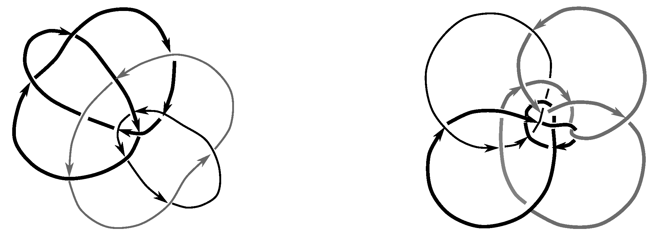
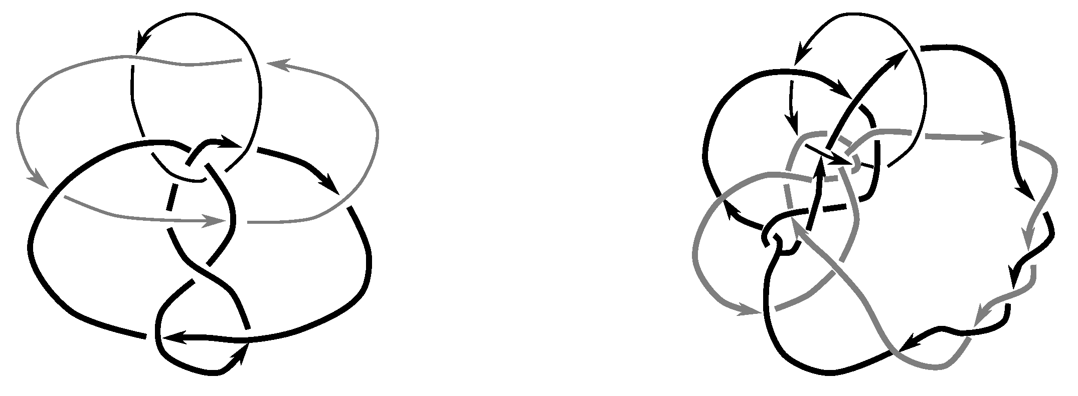
We take the satellites, $L_1,L_2$ of the first and second component of L, for $L\in \{7_6^2,8_{13}^2\}$, as shown in Figure 1 and Figure 2, and then compute the Jones polynomial for each.

$$\begin{array}{cc}\hfill Jones\left({\left(8_{13}^2\right)}_1\right)& =1-\frac{1}{z^6}+\frac{2}{z^5}-\frac{3}{z^4}+\frac{4}{z^3}-\frac{2}{z^2}+\frac{1}{z}-2z+4z^2-2z^3+3z^4-z^5\hfill \\ \hfill Jones\left({\left(8_{13}^2\right)}_2\right)& =1+\frac{1}{z^{11}}-\frac{2}{z^{10}}+\frac{2}{z^8}-\frac{2}{z^7}+\frac{1}{z^6}+\frac{1}{z^5}-\frac{2}{z^4}+\frac{2}{z^3}-\frac{1}{z^2}+\frac{1}{z}-2z+4z^2-z^3+2z^5-z^6\hfill \\ \hfill Jones\left({\left(7_6^2\right)}_1\right)& =2+1/z^{10}-2/z^9+1/z^8-1/z^6+2/z^5-1/z^4+2/z^3-z+z^2+z^3-z^4\hfill \\ \hfill Jones\left({\left(7_6^2\right)}_2\right)& =3+1/z^7-2/z^6+2/z^5-2/z^4+2/z^3+1/z^2-2z+2z^2-z^3\hfill \end{array}$$

Since the Jones polynomials of the two different satellites are not equal for either link L, we have that L is not isotopic to $L_{\gamma }$ for $\gamma =(1,1,1,(12\left)\right)$ by Lemma 6.3. Thus, $(1,1,1,(12\left)\right)\notin \Sigma \left(L\right)$.

Figure C4 and Figure C8 exhibit isotopies that show $(1,-1,1,e)\in \Sigma \left(L\right)$ for both of these links. Therefore, we conclude $\Sigma \left(L\right)={\Sigma }_{4,2}$ for these two links.

7.2.4. Links with Symmetry Group ${\Sigma }_{8,1}$

Claim 7.14

Links $5_1^2$ and $7_3^2$ have symmetry group ${\Sigma }_{8,1}$.

These two links have the pure exchange and pure invertibility symmetries, and their self-writhes are nonzero; thus Lemma 7.6 implies ${\Sigma }_{4,1}<\Sigma \left(L\right)<{\Sigma }_{8,1}$. We show, in Figure B4 and Figure B5, that each symmetry group includes either $(1,1,-1,e)$ or $(1,-1,1,e)$, neither of which is an element of ${\Sigma }_{4,1}$. Therefore, we conclude $\Sigma \left(L\right)={\Sigma }_{8,1}$ for these two links.

7.2.5. Links with Symmetry Group ${\Sigma }_{8,2}$

Claim 7.15

Links $2_1^2,6_2^2,$ and $8_8^2$ have symmetry group ${\Sigma }_{8,2}$.

These three links have the pure exchange and pure invertibility symmetries, and their linking numbers are nonzero; thus Lemma 7.6 implies ${\Sigma }_{4,1}<\Sigma \left(L\right)<{\Sigma }_{8,2}$.

Figure C1, Figure C2, and Figure C5 display the isotopies which show $(-1,1,-1,e)$ lies in the symmetry group for each of these three links. Since this element is not in ${\Sigma }_{4,1}$, we may conclude all three links have symmetry group $\Sigma \left(L\right)={\Sigma }_{8,2}$.

8. Three-Component Links

There are 14 three-component links with 8 or fewer crossings. In this section, we determine the symmetry group for each one; Table 5 summarizes the results. We obtain 11 different symmetry subgroups inside ${\Gamma }_3$, which represent 7 different conjugacy classes of subgroups (out of the 131 possible).

For each link, our first task is to calculate the linking matrix. Then, we utilize

Table 12. This table gives stabilizers for triples in ${\mathbf{Z}}^3$ in the group ${\left({\mathbf{Z}}_2\right)}^3⋊S_3$ under the natural action of this group on ${\mathbf{Z}}^3$. This list of examples covers all the orbit types of this action. As we have shown above, the pre-images of these stabilizers in ${\Gamma }_3$ are the stabilizers of the corresponding linking matrices in $Lk\left(3\right)$. For convenience, the order of these pre-images are given in the right-hand column of the table.

$({\mathbf{Z}}_1,{\mathbf{Z}}_2,{\mathbf{Z}}_3)$	Stabilizer in ${\left({\mathbf{Z}}_2\right)}^3⋊{\mathit{S}}_3$	Stab. in ${\mathbf{\Gamma }}_3$	Order
$(0,0,0)$	${\left({\mathbf{Z}}_2\right)}^3⋊S_3$	${\Gamma }_3$	96
$(a,0,0)$	$(\{+1\}\times {\mathbf{Z}}_2\times {\mathbf{Z}}_2)⋊\{e,\left(23\right)\}$	$D_4\times {\mathbf{Z}}_2$	16
$(a,-a,0)$	$〈(1,1,-1,e),(-1,-1,1,(12\left)\right)〉$	${\left({\mathbf{Z}}_2\right)}^3$	8
$(a,a,0)$	$(\{+1\}\times \{+1\}\times {\mathbf{Z}}_2)⋊\{e,\left(12\right)\}$	${\left({\mathbf{Z}}_2\right)}^3$	8
$(a,b,0)$	$(\{+1\}\times \{+1\}\times {\mathbf{Z}}_2)⋊\left\{e\right\}$	$D_2$	4
$(a,a,-a)$	$S(a,a,-a)$	${\mathbf{Z}}_2\times S_3$	12
$(a,a,a)$	$(\{+1\}\times \{+1\}\times \{+1\})⋊S_3$	${\mathbf{Z}}_2\times S_3$	12
$(a,b,-b)$	$〈(1,-1,-1,(23\left)\right)〉$	$D_2$	4
$(a,b,b)$	$\left(\right\{+1\}\times \{+1\}\times \{+1\left\}\right)⋊\{e,(23\left)\right\}$	$D_2$	4
$(a,b,c)$	$\left\{(1,1,1,e)\right\}$	$D_1$	2

to determine the stabilizer of this matrix within ${\Gamma }_3$; we know that the symmetry group $\Sigma \left(L\right)$ must be a subgroup of this stabilizer. From there, we proceed by ruling out other elements using polynomial invariants and by exhibiting isotopies to show that certain symmetries do lie in $\Sigma \left(L\right)$ until we can discern the symmetry group.

Here are the results, listed in terms of generators for each group. We use the following notation for common group elements:

• PI, for pure invertibility, i.e., the element $(1,-1,-1,-1,e)$
• PE, for having all pure exchanges, i.e., all elements $(1,1,1,1,p)$ where $p\in S_3$

We note that all but two of these links are purely invertible, even though PI might not be part of a minimal set of generators. Neither the Borromean rings $\left(6_2^3\right)$ or the link $8_5^3$ are purely invertible. Both of these links are, however, invertible. The Borromean rings can be inverted using any odd permutation p, i.e., they admit the symmetry $\gamma =(1,-1,-1,-1,p)$; the link $8_5^3$ is invertible using $p=\left(23\right)$.

Claim 8.1

The subgroup $\Sigma \left(6_1^3\right)<{\Gamma }_3$ is the 12 element group isomorphic to $D_6$ generated by pure exchanges and pure invertibility.

The linking matrix for $6_1^3$ is

$$\begin{array}{cccc}& \hfill 1& \hfill 2& \hfill 3\\ 1& \hfill 0& \hfill -1& \hfill -1\\ 2& \hfill -1& \hfill 0& \hfill -1\\ 3& \hfill -1& \hfill -1& \hfill 0\end{array}$$

which is in the standard form $(a,a,a)$. We know that $\Sigma \left(6_1^3\right)$ is a subgroup of the stabilizer of this matrix under the action of ${\Gamma }_3$ on linking matrices. Consulting Table 12, we see that this stabilizer is the group in the claim. We must now show that all these elements are in the group. Figure B2 and Figure D2 show that

$$(1,1,1,1,\left(123\right)),(1,1,1,1,\left(23\right))\in \Sigma \left(6_1^3\right)$$

Since any 3-cycle and 2-cycle generate $S_3$, we have the rest of the pure exchanges as well. Figure D1 shows that this link is purely invertible, completing the proof.

Claim 8.2

The subgroup $\Sigma \left(6_2^3\right)<{\Gamma }_3$ is the 48 element group where $({ϵ}_0,{ϵ}_1,{ϵ}_2,{ϵ}_3,p)$ is in the group if either

(a) 

${ϵ}_1{ϵ}_2{ϵ}_3=1$ and p is an even permutation, or

(b) 

${ϵ}_1{ϵ}_2{ϵ}_3=-1$ and p is odd.

Figure B5, Figure D3, and Figure D4 tell us that $\Sigma \left(6_2^3\right)$ contains the elements

$$(1,-1,1,-1,(132\left)\right),(-1,-1,1,1,(13\left)\right),(-1,1,1,1,e)$$

which clearly obey the rules in the claim. In fact, they generate a group of 48 such elements. Since the order of $\Sigma \left(6_1^3\right)$ must divide $|{\Gamma }_3|=96$, it is either these 48 elements or it is all of ${\Gamma }_3$. But in [21], Montesinos proves that $6_2^3$ is not purely invertible. Thus, $(1,-1,-1,-1,e)$ cannot be in $\Sigma \left(6_2^3\right)$, which completes the proof.

Claim 8.3

The subgroup $\Sigma \left(6_3^3\right)<{\Gamma }_3$ is the 12 element group isomorphic to $D_6$ given by $f^{-1}\left(S(a,a,-a)\right)$.

Figure D5 and Figure D6 imply that $\Sigma \left(6_3^3\right)$ contains

$$\left\{\right(1,1,-1,1,\left(132\right)),(1,-1,-1,-1,\left(12\right)\left)\right\}$$

These three elements generate the 12 element group of the claim. Now the linking matrix for $6_3^3$ is

$$\begin{array}{cccc}& \hfill 1& \hfill 2& \hfill 3\\ 1& \hfill 0& \hfill 1& \hfill -1\\ 2& \hfill 1& \hfill 0& \hfill -1\\ 3& \hfill -1& \hfill -1& \hfill 0\end{array}$$

which is in the standard form $(a,a,-a)$. Consulting Table 12, we see that this means $|\Sigma (6_3^3\left)\right|$ divides 12, the order of the stabilizer. Since we already have 12 elements in the symmetry group, it must equal the stabilizer, which completes the proof.

Claim 8.4

The subgroup $\Sigma \left(7_1^3\right)<{\Gamma }_3$ is the 12 element subgroup isomorphic to $D_6$ that is conjugate to $f^{-1}\left(S(a,a,-a)\right)$ by $(1,1,1,1,(13\left)\right)$.

The linking matrix for $7_1^3$ is

$$\begin{array}{cccc}& \hfill 1& \hfill 2& \hfill 3\\ 1& \hfill 0& \hfill -1& \hfill -1\\ 2& \hfill -1& \hfill 0& \hfill 1\\ 3& \hfill -1& \hfill 1& \hfill 0\end{array}$$

which corresponds to the triple $(1,-1,-1)$ and has the same orbit type as $(a,a,-a)$. Thus, the stabilizer of this linking matrix is a 12 element group conjugate to the stabilizer $f^{-1}\left(S(a,a,-a)\right)$ by $(1,1,1,1,(13\left)\right)$. Figure D7 and Figure D8 show that

$$(1,1,-1,1,\left(123\right)),(1,1,1,1,\left(23\right))\in \Sigma \left(7_1^3\right)$$

These elements generate a 12 element group, so this stabilizer is the entire symmetry group of $7_1^3$, as claimed. We note that this stabilizer was worked out explicitly as Example 5.7.

Claim 8.5

The subgroup $\Sigma \left(8_1^3\right)<{\Gamma }_3$ is the 4 element group isomorphic to $D_2$ generated by pure invertibility and $(1,1,-1,-1,(23\left)\right)$.

The linking matrix for $8_1^3$ is

$$\begin{array}{cccc}& \hfill 1& \hfill 2& \hfill 3\\ 1& \hfill 0& \hfill -1& \hfill 1\\ 2& \hfill -1& \hfill 0& \hfill 2\\ 3& \hfill 1& \hfill 2& \hfill 0\end{array}$$

which is in the standard form $(a,b,-b)$. Consulting Table 12, we see that the stabilizer of this linking matrix in ${\Gamma }_3$ has order 4. But Figure B3 and Figure D9 show stabilizer elements

$$(1,-1,-1,-1,e),(1,-1,1,1,\left(23\right))\in \Sigma \left(8_1^3\right)$$

which means that we also have $(1,1,-1,-1,\left(23\right))\in \Sigma \left(8_1^3\right)$. Therefore these three elements, plus the identity, must form the symmetry group $\Sigma \left(8_1^3\right)$ .

Claim 8.6

The subgroup $\Sigma \left(8_2^3\right)<{\Gamma }_3$ is the 4 element group isomorphic to $D_2$ generated by the pure exchange $(1,1,1,1,(23\left)\right)$ and pure invertibility.

The linking matrix for $8_2^3$ is

$$\begin{array}{cccc}& \hfill 1& \hfill 2& \hfill 3\\ 1& \hfill 0& \hfill -1& \hfill -1\\ 2& \hfill -1& \hfill 0& \hfill -2\\ 3& \hfill -1& \hfill -2& \hfill 0\end{array}$$

which is in the standard form $(a,b,b)$. Consulting Table 12, we see that the stabilizer of $Lk\left(8_2^3\right)$ has order 4. Figure B4 and Figure D10 show

$$(1,-1,-1,-1,\left(23\right)),(1,1,1,1,\left(23\right))\in \Sigma \left(8_2^3\right)$$

and these generate the 4 element subgroup of the claim, which equals the stabilizer.

Claim 8.7

The subgroup $\Sigma \left(8_3^3\right)<{\Gamma }_3$ is the 12 element group isomorphic to $D_6$ generated by pure exchanges and pure invertibility.

The linking matrix for $8_3^3$ is

$$\begin{array}{cccc}& \hfill 1& \hfill 2& \hfill 3\\ 1& \hfill 0& \hfill -1& \hfill -1\\ 2& \hfill -1& \hfill 0& \hfill -1\\ 3& \hfill -1& \hfill -1& \hfill 0\end{array}$$

which is in the form $(a,a,a)$. Consulting Table 12, we see that the stabilizer of $Lk\left(8_3^3\right)$ has order 12, and hence $|\Sigma (8_3^3\left)\right|$ divides 12. Now Figure D12 and Figure D13 show that

$$(1,1,1,1,\left(12\right)),(1,1,1,1,\left(13\right))\in \Sigma \left(8_3^3\right)$$

Since the cycles $\left(12\right)$ and $\left(13\right)$ generate all of $S_3$, we know that all 6 of the pure exchanges are in $\Sigma \left(8_3^3\right)$. Figure D11 shows that $8_3^3$ is purely invertible as well, completing the proof.

Finally, we note that we have encountered this symmetry group before, as $\Sigma \left(6_1^3\right)=\Sigma \left(8_3^3\right)$.

Claim 8.8

The subgroup $\Sigma \left(8_4^3\right)<\Gamma \left(3\right)$ is the 4 element group isomorphic to $D_2$ generated by pure invertibility and $(-1,1,1,1,(12\left)\right)$.

The linking matrix for $8_4^3$ is

$$\begin{array}{cccc}& \hfill 1& \hfill 2& \hfill 3\\ 1& \hfill 0& \hfill 0& \hfill 2\\ 2& \hfill 0& \hfill 0& \hfill -2\\ 3& \hfill 2& \hfill -2& \hfill 0\end{array}$$

which is in the standard form $(a,-a,0)$. Consulting Table 12, we see that the stabilizer of $Lk\left(8_4^3\right)$ is the 8 element group $f^{-1}\left(S(a,-a,0)\right)$, which is generated by $(-1,1,1,-1,e),(-1,1,1,1,(12\left)\right)$, and pure invertibility. Hence, $|\Sigma (8_4^3\left)\right|$ divides 8. Figure B3 and Figure D14 show that the latter two of these generators, namely pure invertibility and $(-1,1,1,1,(12\left)\right)$, are in $\Sigma \left(8_4^3\right)$.

To finish the proof, we now show that the third stabilizer generator $(-1,1,1,-1,e)$ does not lie in the symmetry group. Applying it to $8_4^3$, we get a link with HOMFLYPT polynomial

$$a^4+\frac{1}{a^4}-2a^2{z}^2+\frac{a^2}{z^2}-\frac{2z^2}{a^2}+\frac{1}{a^2{z}^2}+z^4-\frac{2}{z^2}-2$$

However, the base $8_4^3$ has HOMFLYPT polynomial

$$a^2{z}^4+\frac{z^4}{a^2}+3a^2{z}^2+\frac{3z^2}{a^2}+\frac{a^2}{z^2}+\frac{1}{a^2{z}^2}+4a^2+\frac{4}{a^2}-z^6-5z^4-10z^2-\frac{2}{z^2}-8$$

This means that $(-1,1,1,-1,e)\notin \Sigma \left(8_4^3\right)$ and hence that $\Sigma \left(8_4^3\right)$ is generated by $(-1,1,1,1,(12\left)\right)$ and pure invertibility, as claimed.

Claim 8.9

The symmetry group $\Sigma \left(8_5^3\right)<{\Gamma }_3$ is the four element group isomorphic to $D_2$ generated by $(1,1,-1,-1,e)$ and $(1,-1,1,1,(23\left)\right)$.

Figure D15 and Figure D16 imply that the four element group given above is a subgroup of $\Sigma \left(8_5^3\right)$. Now the linking matrix for $8_5^3$ is

$$\begin{array}{cccc}& \hfill 1& \hfill 2& \hfill 3\\ 1& \hfill 0& \hfill 0& \hfill 0\\ 2& \hfill 0& \hfill 0& \hfill -1\\ 3& \hfill 0& \hfill -1& \hfill 0\end{array}$$

which is in the standard form $(a,0,0)$. This means that the symmetry group must be a subgroup of the 16 element pre-image of $\{\{+1\}\times {\mathbf{Z}}_2\times {\mathbf{Z}}_2⋊\{e,\left(23\right)\}$ in ${\Gamma }_3$. Computing this pre-image, we observe next that if we apply any of the group elements

$$\begin{array}{cccc}(-1,-1,-1,1,(23\left)\right)\hfill & (-1,-1,1,-1,(23\left)\right)\hfill & (-1,1,-1,1,(23\left)\right)\hfill & (-1,1,1,-1,(23\left)\right)\hfill \\ (-1,-1,-1,1,e)\hfill & (-1,-1,1,-1,e)\hfill & (-1,1,-1,1,e)\hfill & (-1,1,1,-1,e)\hfill \end{array}$$

in this pre-image to our link, we get a link with Jones polynomial

$$-\frac{1}{z^5}+\frac{3}{z^4}-z^3-\frac{3}{z^3}+3z^2+\frac{6}{z^2}-4z-\frac{5}{z}+6$$

while the base link has Jones polynomial

$$-\frac{1}{z^6}+\frac{3}{z^5}-\frac{4}{z^4}+\frac{6}{z^3}-z^2-\frac{5}{z^2}+3z+\frac{6}{z}-3$$

This rules out those 8 elements, leaving us with a subgroup of 8 possible elements remaining. Interestingly, even framing the various components of the knot and using the satellite lemma does not allow us to rule out any of the remaining symmetries. However, this link is hyperbolic, and Henry and Weeks[3] use SnapPea to show that the symmetry group has four elements. Thus the four element subgroup of $\Sigma \left(8_5^3\right)$ generated by the isotopies in Figure D15 and Figure D16 must be the entire group.

Claim 8.10

The subgroup $\Sigma \left(8_6^3\right)<{\Gamma }_3$ is the 8 element group isomorphic to ${\left({\mathbf{Z}}_2\right)}^3$ which is generated by

$$(1,-1,-1,-1,e),(1,-1,1,1,(23\left)\right),and(-1,1,-1,-1,e)$$

Figure B3, Figure D17, and Figure D18, respectively, imply that the three generators above lie in the symmetry group $\Sigma \left(8_6^3\right)$. Now the linking matrix for $8_6^3$ is

$$\begin{array}{cccc}& \hfill 1& \hfill 2& \hfill 3\\ 1& \hfill 0& \hfill 1& \hfill -1\\ 2& \hfill 1& \hfill 0& \hfill 0\\ 3& \hfill -1& \hfill 0& \hfill 0\end{array}$$

which corresponds to the triple $(0,-1,1)$ and has the same orbit type as $(a,-a,0)$. Consulting Table 12, we see that the stabilizer of the linking matrix is precisely the group above, and hence equals $\Sigma \left(8_6^3\right)$, which completes the proof.

Claim 8.11

The subgroup $\Sigma \left(8_7^3\right)<{\Gamma }_3$ is the 4 element group isomorphic to $D_2$ generated by the pure exchange $(1,1,1,1,(23\left)\right)$ and pure invertibility.

Figure B4 and Figure D19 show that $(1,-1,-1,-1,\left(23\right),(1,1,1,1,\left(23\right))\in \Sigma \left(8_7^3\right)$, which implies that the subgroup above is contained in $\Sigma \left(8_7^3\right)$. Now the linking matrix for $8_7^3$ is

$$\begin{array}{cccc}& \hfill 1& \hfill 2& \hfill 3\\ 1& \hfill 0& \hfill 1& \hfill 1\\ 2& \hfill 1& \hfill 0& \hfill -2\\ 3& \hfill 1& \hfill -2& \hfill 0\end{array}$$

which is in the standard form $(a,b,b)$. Consulting Table 12, we see that $|\Sigma (8_7^3\left)\right|$ divides 4. Since we already have 4 elements in the group, this completes the proof.

Finally, we note that we have encountered this symmetry group before, as $\Sigma \left(8_2^3\right)=\Sigma \left(8_7^3\right)$.

Claim 8.12

The subgroup $\Sigma \left(8_8^3\right)<{\Gamma }_3$ is the four element subgroup isomorphic to $D_2$ generated by pure invertibility and $(1,1,-1,-1,(23\left)\right)$.

Figure D20 and Figure D21 show that $(1,-1,1,1,\left(23\right),(1,1,-1,-1,\left(23\right))\in \Sigma \left(8_8^3\right)$, which implies that $\Sigma \left(8_8^3\right)$ contains the claimed group. Now the linking matrix for $8_8^3$ is

$$\begin{array}{cccc}& \hfill 1& \hfill 2& \hfill 3\\ 1& \hfill 0& \hfill 1& \hfill -1\\ 2& \hfill 1& \hfill 0& \hfill -2\\ 3& \hfill -1& \hfill -2& \hfill 0\end{array}$$

which is in the standard form $(a,b,-b)$. Consulting Table 12, we see that $|\Sigma (8_8^3\left)\right|$ divides 4. This completes the proof, since we already have 4 elements in the subgroup.

Finally, we note that we have encountered this symmetry group before, as $\Sigma \left(8_1^3\right)=\Sigma \left(8_8^3\right)$.

Claim 8.13

The subgroup $\Sigma \left(8_9^3\right)<{\Gamma }_3$ is the 8 element group isomorphic to ${\left({\mathbf{Z}}_2\right)}^3$ generated by pure invertibility, the pure exchange $(1,1,1,1,(23\left)\right)$ and $(1,-1,1,1,e)$.

Figure B4, Figure D22, and Figure D23 show that $(1,-1,-1,-1,\left(23\right),(1,1,1,1,\left(23\right)),(1,-1,1,1,e)\in \Sigma \left(8_9^3\right)$, which implies that the 8 element subgroup generated by these elements is a subgroup of $\Sigma \left(8_9^3\right)$. Now the linking matrix for this link is

$$\begin{array}{cccc}& \hfill 1& \hfill 2& \hfill 3\\ 1& \hfill 0& \hfill 0& \hfill 0\\ 2& \hfill 0& \hfill 0& \hfill 2\\ 3& \hfill 0& \hfill 2& \hfill 0\end{array}$$

which is in the standard form $(a,0,0)$. Consulting Table 12, we see that $|\Sigma (8_9^3\left)\right|$ divides 16. Working out these 16 elements as in the case of $8_5^3$, we see that if we apply any of the elements

$$\begin{array}{cccc}(-1,-1,-1,1,(23\left)\right)\hfill & (-1,-1,1,-1,(23\left)\right)\hfill & (-1,1,-1,1,(23\left)\right)\hfill & (-1,1,1,-1,(23\left)\right)\hfill \\ (-1,-1,-1,1,e)\hfill & (-1,-1,1,-1,e)\hfill & (-1,1,-1,1,e)\hfill & (-1,1,1,-1,e)\hfill \end{array}$$

to $8_9^3$, we get a link with Jones polynomial

$$2z^5-2z^4+4z^3-2z^2+3z+\frac{1}{z}-2$$

while the Jones polynomial of the base $8_9^3$ link is

$$z^7-2z^6+3z^5-2z^4+4z^3-2z^2+2z$$

This leaves only the subgroup claimed. We note that while $Lk\left(8_5^3\right)$ and $Lk\left(8_9^3\right)$ have the same stabilizer, the symmetry group $\Sigma \left(8_5^3\right)$ is a proper subgroup of $\Sigma \left(8_9^3\right)$.

Claim 8.14

The subgroup $\Sigma \left(8_{10}^3\right)<{\Gamma }_3$ is the 4 element group isomorphic to $D_2$ generated by pure invertibility and the pure exchange $(1,1,1,1,(12\left)\right)$.

Figure B3 and Figure D24 show that $(1,-1,-1,-1,e)$ and $(1,1,1,1,(12\left)\right)$ are in $\Sigma \left(8_{10}^3\right)$. Now the linking matrix for $8_{10}^3$ is

$$\begin{array}{cccc}& \hfill 1& \hfill 2& \hfill 3\\ 1& \hfill 0& \hfill 0& \hfill 2\\ 2& \hfill 0& \hfill 0& \hfill 2\\ 3& \hfill 2& \hfill 2& \hfill 0\end{array}$$

which has the standard form $(a,a,0)$. Consulting Table 12, we see that this matrix has an 8 element stabilizer in ${\Gamma }_3$ given by the inverse image of $〈(1,1,1,(12\left)\right),(1,1,-1,e)〉$ under the map f. Now we observe that if we apply any of the four elements

$$\begin{array}{cccc}(-1,-1,-1,1,(12\left)\right)\hfill & (-1,1,1,-1,(12\left)\right)\hfill & (-1,-1,-1,1,e)\hfill & (-1,1,1,-1,e)\hfill \end{array}$$

in this stabilizer to $8_{10}^3$, we get a link with Jones polynomial

$$z^{10}+z^6+z^5+z^3$$

while the base $8_{10}^3$ link has Jones polynomial

$$z^9+z^7+z^6+z^2$$

This rules out all but the four element subgroup above, completing the proof.

9. Isotopies for Four-Component Links

There are three prime four-component links with 8 crossings. They are quite similar in appearance, with only some crossing changes distinguishing them. Their symmetry computations are made somewhat more difficult by the fact that we are working in the 768 element group ${\Gamma }_4$. All three of these links are composed of four unknots linked together so that component 1 is linked to 2 and 3, and 2 and 3 are linked to 4.

Here are the symmetry groups for these links, listed in terms of generators for each group. Again, we denote the purely invertible symmetry, i.e., element $(1,-1,-1,-1,-1,e)$, by PI; all three links admit this symmetry.

Our approach mimics the one used for three-component links. After calculating the linking matrix, we utilize Table 7 to determine the stabilizer of this matrix within ${\Gamma }_4$; we know that the symmetry group $\Sigma \left(L\right)$ must be a subgroup of this stabilizer. Next, we show some elements are in the symmetry group by exhibiting isotopies and rule others out using polynomial invariants until we can discern the symmetry group.

Claim 9.1

The symmetry subgroup for $8_1^4$ is the 16 element group isomorphic to ${\mathbf{Z}}_2\times D_4$ given by the $S^3$-orientation-preserving elements of the inverse image $f^{-1}\left(S(a,a,a,a)\right)$.

The linking matrix for $8_1^4$ is

$$\begin{array}{ccccc}& 1& 2& 3& 4\\ 1& 0& 1& 1& 0\\ 2& 1& 0& 0& 1\\ 3& 1& 0& 0& 1\\ 4& 0& 1& 1& 0\end{array}$$

which corresponds to the standard form $(a,a,a,a)$. By Lemma 5.9, $\Sigma \left(8_1^4\right)$ must be a subgroup of the 32 element stabilizer $f^{-1}\left(S(a,a,a,a)\right)$ of the linking matrix.

Figure E1, Figure E2, and Figure B2 show that pure invertibility and $(1,-1,-1,-1,-1,(23\left)\right)$ and $(1,1,1,1,1,(1342\left)\right)$ are all in $\Sigma \left(8_1^4\right)$. Together, these generate the 16 element group of the claim.

We must show that the 16 $S^3$-orientation-reversing elements of the stabilizer (i.e., elements of the form $(-1,{ϵ}_1,\dots ,{ϵ}_4,p)$) are not in the symmetry group. If we apply any of these 16 elements to the base link, we obtain a link with Jones polynomial

$$-5z^{9/2}+z^{7/2}-z^{5/2}-z^{21/2}+3z^{19/2}-6z^{17/2}+4z^{15/2}-7z^{13/2}+4z^{11/2}$$

But the Jones polynomial of the base $8_1^4$ is

$$4z^{9/2}-6z^{7/2}+3z^{5/2}-z^{3/2}-z^{19/2}+z^{17/2}-5z^{15/2}+4z^{13/2}-7z^{11/2}$$

This rules out all 16 of these remaining elements, which proves the claim.

Claim 9.2

The symmetry subgroup for $8_2^4$ is the 16 element group isomorphic to $D_8$ given by the $S^3$-orientation-preserving elements of $f^{-1}\left(S(a,a,-a,a)\right)$.

The linking matrix for $8_2^4$ is

$$\begin{array}{ccccc}& 1& 2& 3& 4\\ 1& 0& 1& -1& 0\\ 2& 1& 0& 0& 1\\ 3& -1& 0& 0& 1\\ 4& 0& 1& 1& 0\end{array}$$

which corresponds to the standard form $(a,a,-a,a)$ (remember that the ordering of elements given by Equation (4) is not obvious). By Lemma 5.9 the stabilizer of this linking matrix in ${\Gamma }_4$ is a 32 element subgroup isomorphic to ${\mathbf{Z}}_2\times D_8$.

Figure E3 and Figure E4 show that $(1,1,1,-1,1,(14\left)\right)$ and $(1,1,1,1,1,(13\left)\right(24\left)\right)$ are in $\Sigma \left(8_1^4\right)$. Together, these generate the 16 element group of the claim.

We must show that the 16 $S^3$-orientation-reversing elements of the stabilizer (i.e., elements of the form $(-1,{ϵ}_1,\dots ,{ϵ}_4,p)$) are not in the symmetry group. If we apply any of these 16 elements to the base link, we obtain a link with Jones polynomial

$$2z^{9/2}-4z^{7/2}+z^{5/2}-4z^{3/2}-3z^{11/2}+\sqrt{z}-\frac{1}{\sqrt{z}}$$

while the base link has Jones polynomial

$$-4z^{9/2}+z^{7/2}-4z^{5/2}+2z^{3/2}-z^{13/2}+z^{11/2}-3\sqrt{z}$$

This rules out these 16 remaining elements, so the claim is proven.

Claim 9.3

The symmetry subgroup for $8_3^4$ is the 32 element group isomorphic to ${\mathbf{Z}}_2\times {\mathbf{Z}}_2\times D_4$ given by $f^{-1}\left(S(a,-a,-a,a)\right)$.

The linking matrix for $8_3^4$ is

$$\begin{array}{ccccc}& \hfill 1& \hfill 2& \hfill 3& \hfill 4\\ 1& \hfill 0& \hfill 1& \hfill -1& \hfill 0\\ 2& \hfill 1& \hfill 0& \hfill 0& \hfill -1\\ 3& \hfill -1& \hfill 0& \hfill 0& \hfill 1\\ 4& \hfill 0& \hfill -1& \hfill 1& \hfill 0\end{array}$$

which corresponds to the standard form $(a,-a,-a,a)$. By Lemma 5.9 the stabilizer of this linking matrix in ${\Gamma }_4$ is a 32 element subgroup isomorphic to ${\mathbf{Z}}_2\times {\mathbf{Z}}_2\times D_4$. This group is generated by the isotopies in Figure E5, Figure E6, Figure E7, and Figure E8, which show that pure invertibility, along with elements

$$(-1,1,1,1,1,\left(23\right)),(-1,-1,1,1,-1,e),(-1,1,1,1,1,\left(1342\right))\in \Sigma \left(8_3^4\right)$$

10. Comparison of Intrinsic Symmetry Groups with Ordinary Symmetry Groups for Links

We now compare our results on intrinsic symmetry groups to the existing literature on symmetry groups for links. Henry and Weeks [3,22] report $Sym\left(L\right)$ groups for hyperbolic links up to 9 crossings, while Boileau and Zimmerman [4] computed $Sym\left(L\right)$ groups for non-elliptic Montesinos links with up to 11 crossings, and Bonahon and Siebenmann computed $Sym\left(L\right)$ for the Borromean rings link ($6_2^3$) as an example of their methods in [2] (Theorem 16.18).

Comparing all this data with ours, we see that

Lemma 10.1

Among all links of 8 and fewer crossings with known $Sym\left(L\right)$ groups, the Whitten symmetry group $\Sigma \left(L\right)$ is not isomorphic to $Sym\left(L\right)$ only for the links in

Table 13. Among links with 8 or fewer crossings with known $Sym\left(L\right)$ groups, precisely 10 have $\Sigma \left(L\right)\ncong Sym\left(L\right)$.

Link	$\Sigma \left(\mathit{L}\right)$	$|\Sigma (\mathit{L}\left)\right|$	$Sym\left(\mathit{L}\right)$	$|Sym(\mathit{L}\left)\right|$
$6_3^2$	$D_2$	4	${\left({\mathbf{Z}}_2\right)}^3$	8
$8_5^2$	${\mathbf{Z}}_2$	2	$D_2$	4
$8_4^2$	$D_2$	4	${\left({\mathbf{Z}}_2\right)}^3$	8
$8_6^2$	$D_2$	4	${\left({\mathbf{Z}}_2\right)}^3$	8
$8_7^2$	$D_2$	4	${\left({\mathbf{Z}}_2\right)}^3$	8
$8_9^2$	${\mathbf{Z}}_2$	2	$D_2$	4
$8_{11}^2$	${\mathbf{Z}}_2$	2	$D_2$	4
$8_{14}^2$	${\mathbf{Z}}_2$	2	$D_2$	4
$8_{16}^2$	${\mathbf{Z}}_2$	2	${\left({\mathbf{Z}}_2\right)}^3$	8
$8_4^3$	$D_2$	4	$D_4$	8

.

Our results provide some data on symmetry groups of torus links as well.

Lemma 10.2

For the $(2,4)$, $(2,6)$ and $(2,8)$ torus links ($4_1^2$, $6_1^2$, and $8_1^2$), we have $Sym\left(L\right)\simeq \Sigma \left(L\right)\simeq D_2$. For the Hopf link, the $(2,2)$ torus link, we know that $Sym\left(L\right)\simeq \Sigma \left(L\right)\simeq {\left({\mathbf{Z}}_2\right)}^3$.

Goldsmith computed [23] the “motion groups” $M(S^3,L_{(np,nq)})$ for torus knots and links in $S^3$. Combining her Corollary 1.13 and Theorem 3.7, we see that for the $(np,nq)$ torus link $L_{(np,nq)}$, the subgroup ${Sym}^{+}$ of orientation preserving symmetries is homeomorphic to $M(S^3,L_{(np,nq)})$ if $p+q$ is odd, and an index two quotient group of $M(S^3,L_{(np,nq)})$ if $p+q$ is even. The motion group itself is either $D_2$ or an 8-element quaternion group. But in either case ${Sym}^{+}\simeq D_2$.

Now the motion group by itself does not provide any information about the orientation reversing elements in Sym. However, any such element in $Sym\backslash {Sym}^{+}$ would map to an element in $\Sigma \left(L_{(np,nq)}\right)$ which reversed orientation on $S^3$. Since we have already shown that there are no such elements in $\Sigma \left(L_{(np,nq)}\right)$ for $n=1$, $p=1$, $q=2,3,4$, we see that for these links $Sym={Sym}^{+}=\Sigma$. For the Hopf link such an orientation reversing element does exist in $Sym\left(L\right)$. So, $Sym\left(L\right)$ is a $Z_2$ extension of $D_2$ and thus is isomorphic to ${\left({\mathbf{Z}}_2\right)}^3$

By Proposition 4.9, the group $\Sigma \left(L\right)$ is the image of $Sym\left(L\right)$ under a homomorphism, and hence a quotient group of $Sym\left(L\right)$. Further, if $\Sigma \left(L\right)$ has only orientation-preserving elements (on $S^3$) then $Sym\left(L\right)$ does as well. Thus we know something about the $Sym\left(L\right)$ groups of all our links;

Table 14. New results about $Sym\left(L\right)$ symmetry groups: we know from Proposition 4.9 that $\Sigma \left(L\right)$ is a quotient group of $Sym\left(L\right)$. Among the links for which we have computed $\Sigma \left(L\right)$ are a collection of links for which we can find no information in the literature on $Sym\left(L\right)$. Our results imply that the unknown $Sym\left(L\right)$ groups listed above must have a certain quotient.

Link	$|Sym(\mathit{L}\left)\right|$ divisible by	$Sym\left(\mathit{L}\right)$ has quotient
$6_1^3$	12	$D_6$
$6_3^3$	12	$D_6$
$8_6^3$	8	${\left({\mathbf{Z}}_2\right)}^3$
$8_7^3$	4	$D_2$
$8_8^3$	4	$D_2$
$8_9^3$	8	${\left({\mathbf{Z}}_2\right)}^3$
$8_{10}^3$	4	$D_2$

summarizes the new information provided by our approach.

11. Future Directions

We have now presented explicit computations of the Whitten symmetry groups for all links with 8 and fewer crossings. In all the cases we studied, the most difficult part of the computation was obtaining explicit isotopies to generate the symmetry group; ruling out the remaining elements of ${\Gamma }_n$ was generally done by the application of classical invariants. The most difficult of these cases required us to use the “satellite lemma” and study the classical invariants of satellites of our original link.

While we have presented conventional proofs of all our results, we used computer methods extensively in determining the right line of attack for each link—our method was to use the Mathematica package KnotTheory to systematically apply all possible Whitten group elements to each link and then check the knot types of the components, the linking matrix, the Jones polynomial, and the HOMFLYPT polynomial in an attempt to distinguish the new link from the original one. We then checked the computer calculations by hand. This automated method clearly cannot compute $\Sigma \left(L\right)$, but it does provide a subgroup ${\Sigma }^{\prime }\left(L\right)$ of $\Gamma \left(L\right)$ which is known to contain $\Sigma \left(L\right)$. While we do not currently intend to generate isotopies for links with higher crossing number, we intend to present our computationally-obtained ${\Sigma }^{\prime }\left(L\right)$ groups for 9, 10, and 11 crossing links in a future publication.

Some of the most natural questions about the Whitten symmetry groups remain unanswered by this type of explicit enumeration: which groups can arise as Whitten groups? Does every subgroup of a given ${\Gamma }_n$ arise as a $\Sigma \left(L\right)$? We have observed 6 different subgroups of ${\Gamma }_2$, 11 different subgroups of ${\Gamma }_3$, and 3 different subgroups of ${\Gamma }_4$ so far. This subject is certainly worth further exploration: can one generate a carefully chosen link with a given symmetry group?

References and Notes

1. Kodama, K.; Sakuma, M. Symmetry Groups of Prime Knots Up to 10 Crossings. In Knots 90 (Osaka, 1990); Walter de Gruyter: Berlin, Germany, 1992; pp. 323–340. [Google Scholar]
2. Bonahon, F.; Siebenmann, L. New Geometric Splittings of Classical Knots, and the Classification and Symmetries of Arborescent Knots. http://www-bcf.usc.edu/fbonahon/Research/Preprints/Preprints.html (accessed 20 February, 2012).
3. Henry, S.R.; Weeks, J.R. Symmetry groups of hyperbolic knots and links. J. Knot Theory Ramif. 1992, 1, 185–201. [Google Scholar] [CrossRef]
4. Boileau, M.; Zimmermann, B. Symmetries of nonelliptic Montesinos links. Math. Ann. 1987, 277, 563–584. [Google Scholar] [CrossRef]
5. Whitten, W.C., Jr. Symmetries of links. Trans. Am. Math. Soc. 1969, 135, 213–222. [Google Scholar] [CrossRef]
6. Cerf, C. Atlas of oriented knots and links. Top. Atlas 1998, 3, 1–32. [Google Scholar]
7. Doll, H.; Hoste, J. A tabulation of oriented links. Math. Comp. 1991, 57, 747–761. [Google Scholar] [CrossRef]
8. Hillman, J.A. Symmetries of knots and links, and invariants of abelian coverings. I. Kobe J. Math. 1986, 3, 7–27. [Google Scholar]
9. Sakuma, M. Realization of the Symmetry Groups of Links. In Transformation Groups (Osaka, 1987); Springer: Berlin, Germany, 1989; Volume 1375, pp. 291–306. [Google Scholar]
10. Sakuma gives as an explicit example the untwisted double of a two-bridge knot
11. Cantarella, J.; Mastin, M.; Parsley, J. Symmetries of Composite Links, Unpublished work. 2012.
12. Conway, J.H. An Enumeration of Knots and Links, and Some of Their Algebraic Properties. In Computational Problems in Abstract Algebra (Proc. Conf., Oxford, 1967); Pergamon: Oxford, UK, 1970; pp. 329–358. [Google Scholar]
13. Fox, R.H. Some Problems in Knot Theory. In Topology of 3-Manifolds And Related Topics (Proc. The Univ. of Georgia Institute, 1961); Prentice-Hall: Englewood Cliffs, NJ, USA, 1962; pp. 168–176. [Google Scholar]
14. Actually, Fox was willing to call L interchangeable if Σ(L) contained any element in the form (ϵ0,ϵ1,ϵ2,(12)), but we find it more useful to focus on the “pure exchange” symmetry
15. Whitten, W. On prime noninvertible links. Bull. Australian Math. Soc. 1971, 5, 127–130. [Google Scholar] [CrossRef]
16. Culler, M.; Dunfield, N.; University of Illinois at Chicago, Chicago, IL, USA; University of Illinois, Urbana, IL, USA. Private Communication, 2010.
17. SnapPy, 1.3.11; A computer program for studying the geometry and topology of 3-manifolds. http://snappy.computop.org (accessed 20 February, 2012).
18. We had to redraw several links where the component numbering and orientation given by default in SnapPea differed from our choice of numbering and orientation to make the groups agree. The default link data in SnapPea results in several cases in subgroups conjugate to those we give below
19. Murasugi, K. Jones polynomials and classical conjectures in knot theory. II. Math. Proc. Camb. Philos. Soc. 1987, 102, 317–318. [Google Scholar] [CrossRef]
20. Thistlethwaite, M.B. Kauffman’s polynomial and alternating links. Topology 1988, 27, 311–318. [Google Scholar] [CrossRef]
21. Montesinos, J.M. Surgery on Links and Double Branched Covers of S3. In Knots, Groups, and 3-Manifolds (Papers Dedicated to the Memory of R. H. Fox); Princeton Univ. Press: Princeton, NJ, USA, 1975; pp. 227–259. [Google Scholar]
22. Weeks, J.R. Convex hulls and isometries of cusped hyperbolic 3-manifolds. Topol. Appl. 1993, 52, 127–149. [Google Scholar] [CrossRef]
23. Goldsmith, D.L. Motion of links in the 3-sphere. Math. Scand. 1982, 50, 167–205. [Google Scholar] [CrossRef]
Figure 1. Gray knot is satellite for the first and second component of 7 6 2 , respectively.
Symmetry 04 00143 g001
Figure 2. Gray knot is satellite for the first and second component of 8 13 2 , respectively.
Symmetry 04 00143 g002