Characterizations of Network Structures Using Eigenmode Analysis

Abstract

We introduced an analysis to identify structural characterization of two-dimensional regular and amorphous networks. The analysis was shown to be reliable to determine the global network rigidity and can also identify local floppy regions in the mixture of rigid and floppy regions. The eigenmode analysis explores the structural properties of various networks determined by eigenvalue spectra. It is useful to determine the general structural stability of networks that the traditional Maxwell counting scheme based on the statistics of nodes (degrees of freedom) and bonds (constraints) does not provide. A visual characterization scheme was introduced to examine the local structure characterization of the networks. The eigenmode analysis is under development for various practical applications on more general network structures characterized by coordination numbers and nodal connectivity such as graphenes and proteins.

1. Introduction

In nature, all materials can be considered a collection of atoms in specific patterns, and their properties are determined by the interactions between the atoms. The structures of materials, even in continuous limits, can be approximated by discrete nodes and bonds [1,2]. A simple model to describe these properties in the set of many atoms and their interactions would be a network model. Research on the network structures has a long history mostly back to the Lagrange era for mechanical properties [3]. The analogy of network structures to real materials in small scale has been widely employed to address material characterizations both in analytic and computational approaches [3–6]. Mathematical formalisms in many different forms have been developed to predict statistics and kinematics of the networks by solving linear sets of equations of motion [7]. One of the fundamental mathematical analyses has been developed in the form of spectral graph theory to explore the topological characteristics of matrices constructed by nodal connectivity [8,9]. In the network structures, topological connectivity between each structural unit can construct a Laplacian matrix, which includes intrinsic structural information. The spectral analysis on the networks can provide structural stability by determining vibrational modes by matrix diagonalization. Afterwards, many other methods of the eigenmode analysis have been developed originating from the spectral graph theory. However, network analyses in distinct details and application fields shared similarity of their mathematical frameworks, which is originated from the spectral graph theory.

The network models have been successfully employed in various characterizations of materials in nanoscale, and have been investigated due to interest in their applications in mechanical, electrical, and biological devices. It has been shown that the network models in specific atomic arrangements either in certain lattice or in amorphous can reflect most of the nanomaterials in infinitesimal variation limits. The material properties such as structural stability and energetics can be dependent on the specific network structures [10]. For instance, covalent bonds in atomic structures can be strong enough to maintain topology in low temperature regime. Graphenes or proteins can be typical network objects on which the spectral graph theory can be applied to address structural characteristics. One of the widely-known network models would be Gaussian network model (GNM), which decomposes normal modes by the diagonalization of Laplacian (Kirchhoff) matrix. Residual fluctuations and correlations of biomolecules such as B-factor (or Debye-Waller factor) of proteins can be determined by GNM and shown consistent with the X-ray crystallography [11]. It has been generalized to be an isotropic network model (ANM) to determine three-dimensional characteristics of directional preferences [12]. A computationally efficient model called flexibility and rigidity index (FRI) has been recently proposed to determine localized properties of the networks without performing full eigenmode decomposition [13]. The FRI method utilizes only local geometries to determine localized properties such as B-factors in proteins and chemical reactivity in atomic molecules. By utilizing geometry of networks and specific environment, the FRI method is considered highly suitable and efficient for the prediction of localized biological/chemical functions and stabilities.

In this study, we employed a full eigenvalue decomposition method to address the structural characterization of the elastic networks of nanomaterials, such as graphenes not limited to specific biomolecules like proteins, and compared with previous rigidity percolation studies [5,6]. From the numerical analysis, amplitude variations of nodes for eigenvalues (frequencies) were obtained for various lattices and amorphous networks with defects. Due to its intrinsic dynamic nature, the eigenmode analysis provides structural stabilities of the networks in dynamic environment. It was applied to determine global rigidity characterization of the networks, and also to identify local structural characteristics such as floppy and rigid regions. Pristine lattices and inhomogeneous networks with void, topological defects, and bond removals were numerically analyzed to obtain variations of the eigenmode spectra. Using the eigenvalue spectra, structural stability of the networks was visually characterized. Similarly, vibration energy of specific local regions was successfully identified to predict actively responsive to external dynamic inputs. The eigenmode analysis provided insight on geometric effects on the vibrational density of states and structural stability in global scale and local scale as well.

2. Rigidity Analysis

One of the genius characterizations of network stability would be Maxwell counting to determine rigidity of networks [4]. It is based on a simple constraint counting on nodes (degrees of freedom) and bonds (constraints). Extra zero frequencies other than translational and rotational motions of whole body can allow virtual motion without energy variation, which corresponds to floppy modes [5]. Rigidity percolation study is a fascinating subject providing physical understanding on continuous random network models for glasses by relatively simple geometric models [2,5]. As numerical capability to solve large network models is enhanced, various numeric algorithms replace the analytic approach to investigate generalized network models (with defects, amorphous, and complex connectivity). One of the recently developed, simple and fast combinatorial algorithms would be a pebble algorithm originated from ancient children’s play [14]. It was applied to large central-force and bond-bending networks to determine rigidity percolation characteristics and to identify locally floppy, rigid, over-constraint regions. It was shown to agree well with neutron scattering measurement of the density of states [6]. The structural stability sometimes had been investigated in dynamical point of view by considering realistic interactions between the nodes [15]. It can provide more versatile characterization tools, e.g., assessment of network rigidity and mechanical strength which the Maxwell’s constraint counting cannot provide. For rigorous study, until recently, it still requires high computational cost because enormous large set of linear equations should be resolved.

One characteristic of the rigidity of networks would be mechanical strength to resist under certain deformation. A network structure made of nodes and bonds can be characterized by certain geometric parameters, e.g., coordination number and nodal connectivity. Rigidity percolation is a phenomenon that cohesive rigidity occurs for a structure beyond a certain threshold of these parameters. A general network structure can have floppy, rigid, and over-constraint regions [16]. Nodes in the floppy region can freely move without any energy cost in infinitesimal displacement. If the infinitesimal displacement of the nodes changes the energy, it is called rigid. In an over-constraint region, there are more constraints to be marginally rigid.

The network shown in Figure 1 is globally rigid by the Maxwell counting rule with more constraints than the degrees of freedom, but it is noted that the network can have a locally floppy region. Two nodes in the red dotted box are only in the floppy region and the rest nodes in the rest part of the network are completely rigid. It is shown that one can remove a bond without destroying the rigidity of the whole network. For example, the removal of a diagonal bond connecting A and B does not change the structural property of the network. Thus, this bond is an excessive bond in the over-constraint region. It should be noted that the Maxwell counting rule is simply to determine the rigidity, but it does not provide any detail information of locally floppy, rigid, and over-constraint.

Suppose that one may add a bond between C and D, and an over-constraint bond at the center is removed. We can have a completely rigid structure without any locally floppy region. This new network structure has the same number of bonds as the original network. There are four zero-frequency modes for the structure deformation without any energy cost. Two transitional modes and one rotational mode are all trivial modes in two-dimensional networks with open boundary conditions. The one nontrivial zero-frequency mode is determined that for which the floppy region moves horizontally with infinitesimal amount. Here we regard the zero frequency mode is the case where the longitudinal length is not changed for all bonds in the first order approximation.

3. Methodology: Eigenmode Analysis

We employed an eigenmode analysis to investigate structural properties on various types of networks [7,17]. A set of linear Lagrange equations induced for various network structures was constructed and implemented for computational analysis of their eigenmode spectra. The networks consist of nodes with mass and bonds by Hook’s law subject to infinitesimal deformation limits [15]. It was applied to analyze the structural properties and energetics of networks.

3.1. Equation of Motion

The eigenmode analysis has been introduced for the study of normal mode properties of some two-dimensional network structures. For this, we have derived a set of linear equations for small oscillation of d × n coordinates where n is the number of nodes and d is the spatial dimension. In two dimensions (d = 2), we establish a 2n × 2n matrix with the coefficients of these linear equations and, hence, the normal mode vibrations were investigated in two-dimensional networks. Force equation for i-th node exerted by j-th node for the updated positions $\left({\overrightarrow{r}}_i,{\overrightarrow{r}}_j\right)$ of two nodes from the initial positions $\left({\overrightarrow{r}}_{i,0},{\overrightarrow{r}}_{j,0}\right)$ is given by

$${\overrightarrow{F}}_{ij}=-k_{ij}\left(\left|{\overrightarrow{r}}_i-{\overrightarrow{r}}_j\right|-\left|{\overrightarrow{r}}_{i,0}-{\overrightarrow{r}}_{j,0}\right|\right)\frac{\left({\overrightarrow{r}}_i-{\overrightarrow{r}}_j\right)}{\left|{\overrightarrow{r}}_i-{\overrightarrow{r}}_j\right|}$$

(1)

where $k_{ij}$ is the spring constant of the bond between i-th and j-th node. For small displacements of ${\overrightarrow{d}}_i={\overrightarrow{r}}_i-{\overrightarrow{r}}_{i,0}$ and some derivations under the first order approximation, this becomes

$${\overrightarrow{F}}_{ij}=-k_{ij}\frac{{\overrightarrow{L}}_{ij,0}}{L_{ij,0}^2}\left({\overrightarrow{L}}_{ij,0}\cdot {\overrightarrow{d}}_{ij}\right)$$

(2)

where ${\overrightarrow{L}}_{ij,0}={\overrightarrow{r}}_{i,0}-{\overrightarrow{r}}_{j,0}$ and ${\overrightarrow{d}}_{ij}={\overrightarrow{d}}_i-{\overrightarrow{d}}_j.$ All nodes in a normal mode are subject to vibrate with the same resonant frequency ω from the equilibrium positions as the following (only x-component is under investigation and y-component is in the same form)

$$d_i^x\left(t\right)={\mathrm{A}}_{ix}\sin \mathrm{\omega }t$$

(3)

Then, the equation of motion of the x-component of the i-th node ( $d_i^x$) surrounded by the j-th nodes is represented by

$$m_i{\mathrm{\omega }}^2{d}_i^x=-{\displaystyle \sum }_j{k}_{ij}\frac{L_{ij,0}^x}{L_{ij,0}^2}\left({\overrightarrow{L}}_{ij,0}\cdot {\overrightarrow{d}}_{ij}\right)$$

(4)

Here, $m_i$ is the mass of the i-th node and all $m_i$ are considered equal as M. For the spring constant, $k_{ij}=k_{ji}$ in general. The matrix form of the linear equations is represented by

$${\mathrm{M}\mathrm{\omega }}^2\left(\begin{array}{c}{d}_i^x\\ d_i^y\end{array}\right)=-\left(\begin{array}{cc}{\mathrm{M}}_{xx}& {\mathrm{M}}_{xy}\\ {\mathrm{M}}_{yx}& {\mathrm{M}}_{yy}\end{array}\right)\left(\begin{array}{c}{d}_i^x\\ d_i^y\end{array}\right)$$

(5)

where

$${\mathrm{M}}_{xx}=\left[\begin{array}{ccc}\begin{array}{cc}{\displaystyle \sum _j^{\langle nn\rangle }{\mathrm{\eta }}_{1j}{k}_{1j}\frac{L_{1j,0}^x{}^2}{L_{1j,0}{}^2}}& -{\mathrm{\eta }}_{12}{k}_{12}\frac{L_{12,0}^x{}^2}{L_{12,0}{}^2}\\ -{\mathrm{\eta }}_{21}{k}_{21}\frac{L_{21,0}^x{}^2}{L_{21,0}{}^2}& {\displaystyle \sum _j^{\langle nn\rangle }{\mathrm{\eta }}_{2j}{k}_{2j}\frac{L_{2j,0}^x{}^2}{L_{2j,0}{}^2}}\end{array}& \cdots & \begin{array}{c}-{\mathrm{\eta }}_{1n}{k}_{1n}\frac{L_{1n,0}^x{}^2}{L_{1n,0}{}^2}\\ -{\mathrm{\eta }}_{2n}{k}_{2n}\frac{L_{2n,0}^x{}^2}{L_{2n,0}{}^2}\end{array}\\ ⋮& \ddots & ⋮\\ \begin{array}{cc}-{\mathrm{\eta }}_{n1}{k}_{n1}\frac{L_{n1,0}^x{}^2}{L_{n1,0}{}^2}& -{\mathrm{\eta }}_{n2}{k}_{n2}\frac{L_{n2,0}^x{}^2}{L_{n2,0}{}^2}\end{array}& \cdots & {\displaystyle \sum _j^{\langle nn\rangle }{\mathrm{\eta }}_{nj}{k}_{nj}\frac{L_{nj,0}^x{}^2}{L_{nj,0}{}^2}}\end{array}\right]$$

(6)

and

$${\mathrm{M}}_{xy}=\left[\begin{array}{ccc}\begin{array}{cc}{\displaystyle \sum _j^{\langle nn\rangle }{\mathrm{\eta }}_{1j}{k}_{1j}\frac{L_{1j,0}^x{L}_{1j,0}^y}{L_{1j,0}{}^2}}& -{\mathrm{\eta }}_{12}{k}_{12}\frac{L_{12,0}^x{L}_{12,0}^y}{L_{12,0}{}^2}\\ -{\mathrm{\eta }}_{21}{k}_{21}\frac{L_{21,0}^x{L}_{21,0}^y}{L_{21,0}{}^2}& {\displaystyle \sum _j^{\langle nn\rangle }{\mathrm{\eta }}_{2j}{k}_{2j}\frac{L_{2j,0}^x{L}_{2j,0}^y}{L_{2j,0}{}^2}}\end{array}& \cdots & \begin{array}{c}-{\mathrm{\eta }}_{1n}{k}_{1n}\frac{L_{1n,0}^x{L}_{1n,0}^y}{L_{1n,0}{}^2}\\ -{\mathrm{\eta }}_{2n}{k}_{2n}\frac{L_{2n,0}^x{L}_{2n,0}^y}{L_{2n,0}{}^2}\end{array}\\ ⋮& \ddots & ⋮\\ \begin{array}{cc}-{\mathrm{\eta }}_{n1}{k}_{n1}\frac{L_{n1,0}^x{L}_{n1,0}^y}{L_{n1,0}{}^2}& -{\mathrm{\eta }}_{n2}{k}_{n2}\frac{L_{n2,0}^x{L}_{n2,0}^y}{L_{n2,0}{}^2}\end{array}& \cdots & {\displaystyle \sum _j^{\langle nn\rangle }{\mathrm{\eta }}_{nj}{k}_{nj}\frac{L_{nj,0}^x{L}_{nj,0}^y}{L_{nj,0}{}^2}}\end{array}\right]$$

(7)

Here, M_yy and M_yx can be determined in a similar manner with M_xx and M_xy. The sum of ${\displaystyle \sum }_{\mathrm{j}}^{nn}{\text{Element}}_{ij}$ for i-th node is taken for all connected node (j). In the matrices ${\mathrm{\eta }}_{ij}$ is 1 when two nodes of i and j are connected and 0 otherwise. These matrices are sparse because only the nearest neighbors are connected.

Solutions of the above Equation (5) can describe entire normal mode motions of the network system. Eigenmodes with zero eigenvalue, equivalently zero frequency, are those which require no energy for the vibrational motions. Under open boundary conditions, there are three trivial modes, two translational modes and one rotational mode. Under a periodic boundary condition, the rotational mode does not exist. If there are zero energy modes other than these trivial modes, they are floppy modes of the network structure and show that the network is floppy. Here, it should be noted that if the network contains a single locally floppy region, the analysis generates zero energy mode and the network is considered floppy. Thus, it may not distinguish global rigidity and local rigidity. However, as we observed in Figure 1, it is possible for globally rigid network to possess a locally floppy region. Since the global rigidity (or structural stability) might be crucial in many real structural applications, one leaves this study for an important future work.

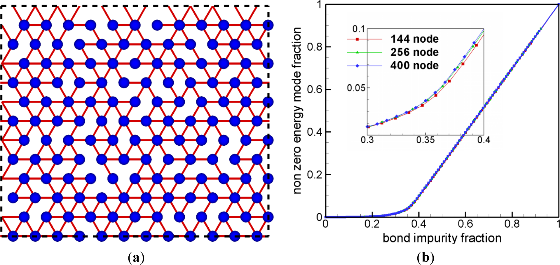
Figure 2a shows a triangular network with randomly removed bonds. Before one removes any bond, the perfect triangular network is completely rigid, and, hence, the number of nontrivial zero energy mode is zero. One may expect that as more bonds are removed, the number of nontrivial zero energy modes increases. If nearly all bonds are removed, that is, all nodes are nearly independent, the number of nontrivial zero energy modes reaches its maximum value and this result is shown in Figure 2b. Obviously, this agrees with the results of previous studies including the pebble game algorithm. The value of bond impurity fraction, at which the second derivative of the nonzero energy mode fraction with respect to the bond impurity fraction reaches the maximum value, is the threshold of the rigidity percolation for this structure. The value of the fraction of connected bonds is reported as 0.66 from the previous studies [6], and the result from our eigenmode analysis on relatively small sized samples is shown to be well matched with the prediction.

3.2. Nodal Amplitude

Normal mode behavior of a network structure is well represented by the eigenvalue distribution. Since the eigenvalue is a square of the normal mode frequency, the eigenvalue distribution shows some aspects such as the bandwidth, that is, the maximum frequency and the probability distribution of the frequencies, which is related to the degeneracy of the specific eigenvalue. As in our previous studies [7,17], the eigenvalue distribution, that is, the vibrational density of states can be represented by a continuous form as a sum of Gaussian functions as Equation (8). The width of the Gaussian function σ is arbitrarily chosen and each Gaussian function represents a single eigenmode and, therefore, eigenvalues with large degeneracies are represented with high peaks.

$$\mathrm{g}\left(\mathrm{\lambda },\mathrm{\sigma }\right)=\frac{1}{2n\mathrm{\sigma }\sqrt{2\mathrm{\pi }}}{\displaystyle \sum }_{i=1}^{2n}\exp \left(-{\left(\mathrm{\lambda }-{\mathrm{\lambda }}_i\right)}^2/2{\mathrm{\sigma }}^2\right)$$

(8)

For each normal mode, the nodes in the network structure vibrate in some patterns and with certain amplitudes. In order to represent a normal mode in two-dimensional structure with n nodes, we have 2n amplitudes. Therefore, for a given eigenvalue $\mathrm{\lambda }$ and node j, there are two amplitudes in two directions, ${\mathrm{A}}_{j,x}\left(\mathrm{\lambda }\right)$ and ${\mathrm{A}}_{j,y}\left(\mathrm{\lambda }\right)$. The two amplitudes in each axis can be combined to a radial amplitude ${\mathrm{A}}_{j,r}\left(\mathrm{\lambda }\right)$ as follows:

$${\mathrm{A}}_{j,r}^2\left(\mathrm{\lambda }\right)={\mathrm{A}}_{j,x}^2\left(\mathrm{\lambda }\right)+{\mathrm{A}}_{j,y}^2\left(\mathrm{\lambda }\right)$$

(9)

This radial amplitude ${\mathrm{A}}_{j,r}\left(\mathrm{\lambda }\right)$ is the level of the motion of j-th node at the normal mode with the eigenvalue $\mathrm{\lambda }$. In order to represent this in a continuous form, we multiply ${\mathrm{A}}_{j,r}\left(\mathrm{\lambda }\right)$ by the Gaussian function $\mathrm{g}\left(\mathrm{\lambda },\mathrm{\sigma }\right)$ as

$$f_j\left(\mathrm{\lambda }\right)={\mathrm{A}}_{j,r}^2\left(\mathrm{\lambda }\right)\mathrm{g}\left(\mathrm{\lambda },\mathrm{\sigma }\right)$$

(10)

While the above represents the response of the j-th node to the normal mode with certain eigenvalue $\mathrm{\lambda }$, one may want the response of the node to many normal modes with the eigenvalues within a certain domain ${\mathrm{\lambda }}_{\mathrm{a}}~{\mathrm{\lambda }}_{\mathrm{b}}$. We just sum the value in the Equation (10) over this eigenvalue domain as follows:

$$F_j\left({\mathrm{\lambda }}_{\mathrm{a}},{\mathrm{\lambda }}_{\mathrm{b}}\right)=\underset{{\mathrm{\lambda }}_{\mathrm{a}}}{\overset{{\mathrm{\lambda }}_{\mathrm{b}}}{{\displaystyle \int }}}{\mathrm{A}}_{j,r}^2\left(\mathrm{\lambda }\right)\mathrm{g}\left(\mathrm{\lambda },\mathrm{\sigma }\right)\mathrm{d}\mathrm{\lambda }$$

(11)

This is a form of amplitude spectrum of the j-th node, which represents how the level of the motion of j-th node changes according to the eigenvalue in this domain of the eigenvalue. For the full amplitude spectrum, we set

$$F_j\left({\mathrm{\lambda }}_1,{\mathrm{\lambda }}_{2\mathrm{n}}\right)=\underset{{\mathrm{\lambda }}_1}{\overset{{\mathrm{\lambda }}_{2\mathrm{n}}}{{\displaystyle \int }}}{\mathrm{A}}_{j,r}^2\left(\mathrm{\lambda }\right)\mathrm{g}\left(\mathrm{\lambda },\mathrm{\sigma }\right)\mathrm{d}\mathrm{\lambda }$$

(12)

4. Structural Analysis

The radial amplitude can be simultaneously determined for all nodes in the network structure. By calculating and showing a scalar value for all nodes, one can show certain properties for the structure. One can add up squared values of radial amplitude for an eigenvalue domain as follows:

$${\mathrm{F}}_j\left({\mathrm{\lambda }}_1,{\mathrm{\lambda }}_2\right)={\displaystyle \sum }_{\mathrm{\lambda }={\mathrm{\lambda }}_1}^{{\mathrm{\lambda }}_2}{\mathrm{A}}_{j,r}^2\left(\mathrm{\lambda }\right)$$

(13)

This value ${\mathrm{F}}_j\left({\mathrm{\lambda }}_1,{\mathrm{\lambda }}_2\right)$ can be calculated for all node j and be shown together in order to represent node responses for the eigenvalue range of ${\mathrm{\lambda }}_1~{\mathrm{\lambda }}_2$. We will call this quantity as a squared amplitude sum.

With this squared amplitude sum, we can identify individual node or set of the nodes which are more reactive under external dynamic inputs with a certain range of eigenvalue.

4.1. Triangular Network with Bond Defects

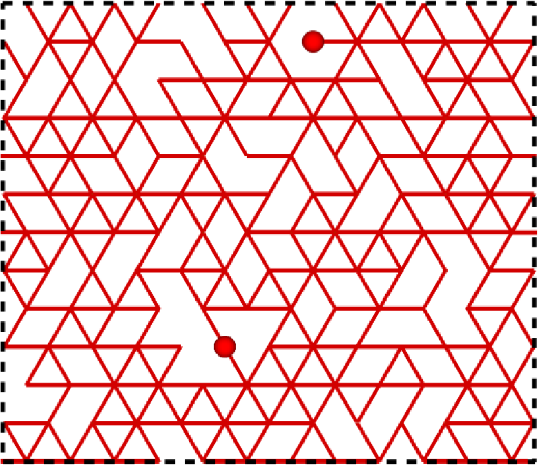
In a network structure, the floppy region costs no energy to be deformed while others cost a certain amount of energy. If we choose the eigenvalue domain only for zero eigenvalue, we may find the floppy regions with the squared amplitude sum. Other than the trivial modes such as translational modes, only nodes in floppy regions may move for zero eigenvalues, that is, for zero energy modes. In general, there are degeneracies for zero eigenvalue and there are many zero energy modes other than the trivial modes for large networks. Therefore, the squared amplitude sum for zero eigenvalue has much larger value for nodes in floppy regions than for the rests. Figure 3 shows the triangular network with randomly removed bonds. All nodes in the network have the same mass and the spring constant is uniform. In the figure, the size of the node denotes the squared amplitude sum for zero eigenvalue. Only two nodes show large amplitude for the zero energy modes representing floppy nodes. This method can be applied not only for zero energy modes but also for the finite energy modes. By calculating this squared amplitude sum for various eigenvalue domains, one can find structural properties of a network regarding normal mode dynamics.

4.2. Randomized Hexagonal Networks

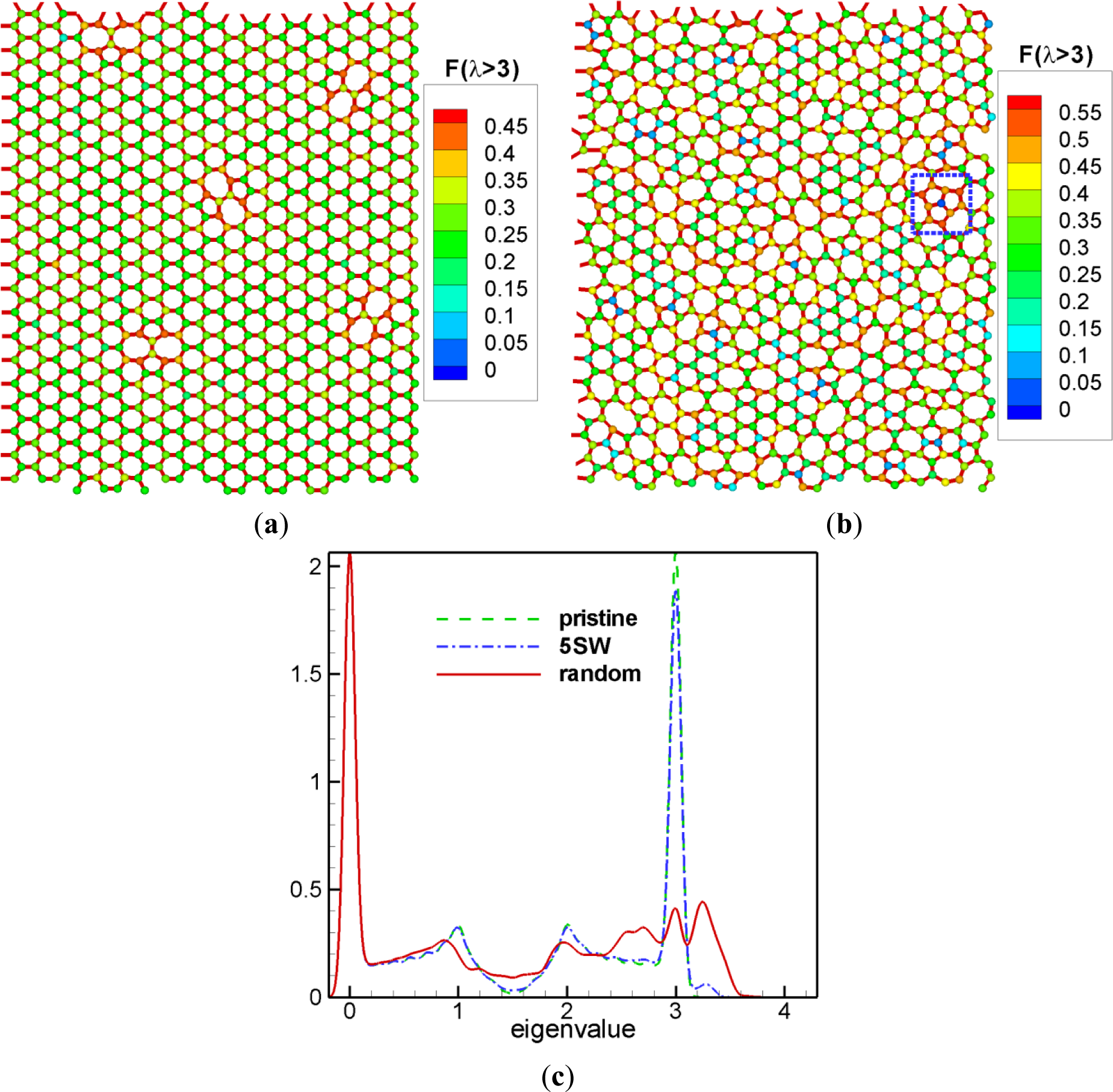
As mentioned earlier, the squared amplitude sum for higher eigenvalue domains enables us to determine stiffer regions. Nodes in these regions are more responsive for normal modes with higher eigenvalues. Here we introduce a hexagonal lattice network as an illustrative example. Two-dimensional hexagonal network is geometrically identical to the graphene in real world [18]. Numerous characterizations were performed on the superior properties of the graphenes with realistic defects. One of the typical defects in graphene is the Stone-Wales defect [19,20]. Figure 4a shows a structure of 800 node hexagonal network with five Stone-Wales defects. Here, we calculated the amplitude sum for the eigenvalues larger than 3.0, ${\mathrm{F}}_j\left(\mathrm{\lambda }>3\right)$ and showed as the color for all nodes. Nodes with large values of ${\mathrm{F}}_j\left(\mathrm{\lambda }>3\right)$ are mostly in the Stone-Wales defects and nearly all other nodes have very small values of ${\mathrm{F}}_j\left(\mathrm{\lambda }>3\right)$ except for a few. In addition, these few nodes are all rather close to the defects. The reason to choose the eigenvalues above 3.0 is that adding these Stone-Wales defects to the hexagonal network creates eigenvalues above 3.0 as shown in Figure 4c. Figure 4c represents the vibrational density of states for various networks plotted with the sum of the Gaussian function $\mathrm{g}\left(\mathrm{\lambda },\mathrm{\sigma }\right)$ with $\mathrm{\sigma }=0.05$ according to Equations (8) and (12) [17].

By adding more Stone-Wales defects and relaxing with molecular dynamics, one can get a random network as shown in Figure 4b [1,5,17] and here we also showed the squared amplitude sum ${\mathrm{F}}_j\left(\mathrm{\lambda }>3\right)$. Nodes with large values of ${\mathrm{F}}_j\left(\mathrm{\lambda }>3\right)$ are distributed in an irregular pattern; however, we find these are located near the regions with more deformed local structure. Especially, nodes in the square box have highest values of ${\mathrm{F}}_j\left(\mathrm{\lambda }>3\right)$ and three pentagons are neighboring here, that is, this is the mostly deformed region. The center point where these three pentagons meet has a very small value of ${\mathrm{F}}_j\left(\mathrm{\lambda }>3\right)$. Normal modes with $\mathrm{\lambda }>3$ create radial motions of nodes in each pentagon, and the destructive interference of these three radial motions at a given frequency destroyed the amplitude of the center node. From Figure 4c, one can see that there are a lot more eigenvalues larger than 3.0 for the random network than for the network with five Stone-Wales defects. This is consistent with the fact that there are more deformed regions and more nodes are involved with the motions with the eigenvalues larger than 3.0.

5. Energy Analysis

While the squared amplitude sum describes the dynamic property of a network for a specified eigenvalue range, one may need a more universal quantity obtained through whole eigenvalue domain to describe overall network properties. One can try to add up the amplitude sum for all eigenvalues ${\mathrm{\lambda }}_1$ to ${\mathrm{\lambda }}_{2n}$, that is, ${\mathrm{F}}_j\left({\mathrm{\lambda }}_1,{\mathrm{\lambda }}_{2n}\right)$. From Equations (9) and (12)

$${\mathrm{F}}_j\left({\mathrm{\lambda }}_1,{\mathrm{\lambda }}_{2\mathrm{n}}\right)={\displaystyle \sum }_{\mathrm{\lambda }={\mathrm{\lambda }}_1}^{{\mathrm{\lambda }}_{2n}}{\mathrm{A}}_{j,r}^2\left(\mathrm{\lambda }\right)={\displaystyle \sum }_{\mathrm{\lambda }={\mathrm{\lambda }}_1}^{{\mathrm{\lambda }}_{2n}}\left({\mathrm{A}}_{j,x}^2\left(\mathrm{\lambda }\right)+{\mathrm{A}}_{j,y}^2\left(\mathrm{\lambda }\right)\right)$$

(14)

And this is a sum of squared amplitudes of two orthonormal eigenvectors and hence is just two in any case.

$${\mathrm{C}}_j\left({\mathrm{\lambda }}_1,{\mathrm{\lambda }}_{2n}\right)={\displaystyle \sum }_{\mathrm{\lambda }={\mathrm{\lambda }}_1}^{{\mathrm{\lambda }}_{2n}}{\mathrm{A}}_{j,r}^2\left(\mathrm{\lambda }\right)\mathrm{\lambda }$$

(15)

In the above Equation (15), $\mathrm{\lambda }$ is multiplied to the squared amplitudes before we sum up. We will consider this quantity as an averaged eigenvalue. For a normal mode in a system with uniform mass for all nodes, $m=1$ and $\mathrm{\lambda }={\mathrm{\omega }}^2=k$. Then, the above has a form of ${\displaystyle \sum {\mathrm{A}}_{j,r}^2\left(\mathrm{\lambda }\right)k}$ and has a meaning of a sum of energy stored in the springs connected to the j-th node. Unless the network is uniform both for the coordination number and the spring constant, this quantity ${\mathrm{C}}_j\left({\mathrm{\lambda }}_1,{\mathrm{\lambda }}_{2n}\right)$ is nontrivial. By calculating this value for all nodes, one can show an energy contour to describe certain network properties.

5.1. Triangular Network with Bond Removals

Figure 5 shows a triangular network with randomly removed bonds and the averaged eigenvalue ${\mathrm{C}}_j\left({\mathrm{\lambda }}_1,{\mathrm{\lambda }}_{2n}\right)$ denoted for all nodes. This network has uniform spring constants, and the nodes have various coordination numbers varying from one to six. As one might conjecture, the averaged eigenvalue is the coordination number in this case since ${\mathrm{C}}_j\left({\mathrm{\lambda }}_1,{\mathrm{\lambda }}_{2n}\right)$ has a sense of sum of spring energy connected to a j-th node mention above.

5.2. Hexagonal Networks

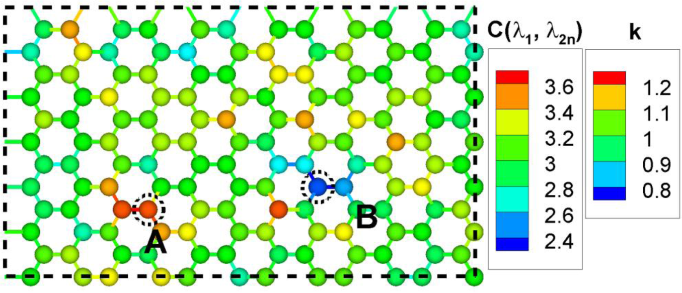
Figure 6 shows a hexagonal network with inhomogeneous spring constants with Gaussian distribution $\Delta k/k=0.1$. The homogeneous spring constant case is rather trivial, that is, the averaged eigenvalue ${\mathrm{C}}_j\left({\mathrm{\lambda }}_1,{\mathrm{\lambda }}_{2n}\right)$ would be three for all nodes, but this inhomogeneous case is different. Nodes connected with springs with higher spring constant have higher values of ${\mathrm{C}}_j\left({\mathrm{\lambda }}_1,{\mathrm{\lambda }}_{2n}\right)$. Regions containing these nodes are stiffer and have more mechanical energy stored. Similarly, nodes connected with springs with lower spring constant have lower values of ${\mathrm{C}}_j\left({\mathrm{\lambda }}_1,{\mathrm{\lambda }}_{2n}\right)$. Node A and B have highest and lowest values of ${\mathrm{C}}_j\left({\mathrm{\lambda }}_1,{\mathrm{\lambda }}_{2n}\right)$, respectively.

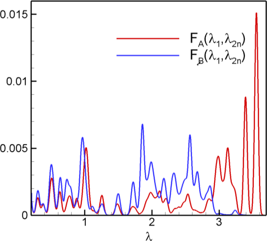
For these extreme nodes A and B, Figure 7 shows the amplitude spectra ${\mathrm{F}}_j\left({\mathrm{\lambda }}_1,{\mathrm{\lambda }}_{2n}\right)$ in Equation (12). ${\mathrm{F}}_{\mathrm{A}}\left({\mathrm{\lambda }}_1,{\mathrm{\lambda }}_{2n}\right)$ has a large value for high eigenvalues and a small value for middle and low eigenvalues. ${\mathrm{F}}_{\mathrm{B}}\left({\mathrm{\lambda }}_1,{\mathrm{\lambda }}_{2n}\right)$ has very small value for high eigenvalues and large value for middle and low eigenvalues. The amplitude spectra ${\mathrm{F}}_j\left({\mathrm{\lambda }}_1,{\mathrm{\lambda }}_{2n}\right)$ represent physically more active frequencies and less active frequencies for a specific node.

6. Conclusions

In this study, we have investigated various network properties by using the eigenmode analysis. A full eigenvalue decomposition scheme was introduced to explore structural information of the networks in a wide range of normal modes. This method was shown to determine and visualize various characteristics of normal modes for specific frequency ranges or a full range of spectrums. By using the amplitude analysis, we were able to identify floppy regions in a network without energy cost under infinitesimal deformations. For this, we searched those regions containing nodes with large amplitudes for the zero eigenvalue. By searching the same for higher eigenvalues, more deformed regions were visually identified for the Stone-Wales defects added on the hexagonal network and the random network. In general, with this structural analysis, we can find dynamic response behavior of the networks for normal modes in any frequency domain. Along with the change of the network structure such as adding structural impurities and random networks, inhomogeneity of the spring constant is also a possible generalization for the network problem. The energy analysis was utilized for this problem and hence an energy contour map was visualized.

It is clear that our eigenmode analysis may be implemented to calculate the vibrational density of states for a given system, which is comparable to the phonon spectrum by experiments such as Raman spectroscopy and other calculation methods [21]. Introducing longer-range bonds and angular force terms may be possible along with various structures with different masses to simulate real materials. Unlike the quantum mechanical calculations, our method has the capability to explore much larger sizes of the system. This is because one can solve the eigenvalue problem for tens of thousands of matrix dimensions even without using the sparse matrix technique [22]. The amplitude spectrum may replace the vibrational density of states in order to investigate the locality dependence of the structural property. Hence, this enables us to predict certain results of some other methods.

References

- Zallen, R. The Physics of Amorphous Solids; John Wiley & Sons: New York, NY, USA, 1983. [Google Scholar]
- Phillips, J.C. Topology of covalent non-crystalline solids, II. Medium-range order in chalcogenide alloys and A-Si(Ge). J. Non-Cryst. Solids 1981, 43, 37–77. [Google Scholar]
- Lagrange, J.L. Analytical Mechanics, novella edition of 1811; Boissonnade, A., Vagliente, V.N., Eds.; Springer: Dordrecht, The Netherlands, 1997; translated from the Mécanique Analytique. [Google Scholar]
- Maxwell, J.C. On reciprocal figures and diagrams of forces. Philos. Mag. 1864, 27, 294–299. [Google Scholar]
- Thorpe, M.F. Continuous deformations in random networks. J. Non-Cryst. Solids 1983, 57, 355–370. [Google Scholar]
- Jacobs, D.J.; Thorpe, M.F. Generic rigidity percolation: The pebble game. Phys. Rev. Lett. 1995, 75, 4051–4054. [Google Scholar]
- Park, Y.; Hyun, S.; Kang, K.-J. Structural analysis on kagome trusses under dynamic external loadings. J. Korean Phys. Soc. 2012, 60, 349–355. [Google Scholar]
- Ivanciuk, O.; Balaban, A.T. Encyclopedia of Computational Chemistry, Graph Theory in Chemistry; Schleyer, P.V.R., Ed.; John Wiley & Sons: New York, NY, USA, 1998; Volume 2. [Google Scholar]
- Vishveshwara, S.; Brinda, K.V.; Kannan, N. Protein structure: Insights from graph theory. J. Theor. Comput. Chem. 2002, 1. [Google Scholar] [CrossRef]
- Ashby, M.F.; Gibson, L.J. Cellular Solids: Structure & Properties, 2nd ed; Cambridge University: New York, NY, USA, 1997. [Google Scholar]
- Haliloglu, T.; Bahar, I.; Erman, B. Gaussian dynamics of folded proteins. Phys. Rev. Lett. 1997, 79. [Google Scholar] [CrossRef]
- Atilgan, A.R.; Durell, S.R.; Jernigan, R.L.; Demirel, M.C.; Keskin, O.; Bahar, I. Anisotropy of fluctuation dynamics of proteins with an elastic network model. Biophys. J. 2001, 80, 505–515. [Google Scholar]
- Xia, K.; Opron, K.; Wei, G.-W. Multiscale multiphysics and multidomain models—Flexibility and rigidity. J. Chem. Phys. 2013, 139. [Google Scholar] [CrossRef]
- Jacobs, D.J.; Hendrickson, B. An algorithm for two-dimensional rigidity percolation: The pebble game. J. Comp. Phys. 1997, 137, 346–365. [Google Scholar]
- Kirkwood, J.G. The dielectric polarization of polar liquids. J. Chem. Phys. 1939, 7. [Google Scholar] [CrossRef]
- Thorpe, M.F. Bulk and surface floppy modes. J. Non-Cryst. Solids 1995, 182, 135–142. [Google Scholar]
- Park, Y.; Hyun, S. Vibrational characterization of two-dimensional networks: Effects of patterns and defects. J. Korean Phys. Soc. 2014, 64, 786–794. [Google Scholar]
- Geim, A.K.; Novoselov, K.S. The rise of grapheme. Nat. Mater. 2007, 6, 183–191. [Google Scholar]
- Stone, A.J.; Wales, D.J. Theoretical studies of icosahedral C60 and some related species. Chem. Phys. Lett. 1986, 128, 501–503. [Google Scholar]
- Tuan, D.V.; Kumar, A.; Roche, S.; Ortmann, F.; Thorpe, M.F.; Ordejon, P. Insulating behavior of an amorphous graphene membrane. Phys. Rev. B 2012, 86. [Google Scholar] [CrossRef]
- Maola, S.; Häkkinen, H.; Koskinen, P. Comparison of Raman spectra and vibrational density of states between graphene nanoribbons with different edges. Eur. Phys. J. D 2009, 52, 71–74. [Google Scholar]
- Saad, Y. Numerical Methods for Large Eigenvalue Problems: Theory and Algorithms; Wiley: New York, NY, USA, 1992. [Google Scholar]
© 2015 by the authors; licensee MDPI, Basel, Switzerland This article is an open access article distributed under the terms and conditions of the Creative Commons Attribution license (http://creativecommons.org/licenses/by/4.0/).
Share and Cite
Park, Y.; Hyun, S. Characterizations of Network Structures Using Eigenmode Analysis. Symmetry 2015, 7, 962-975. https://doi.org/10.3390/sym7020962
Park Y, Hyun S. Characterizations of Network Structures Using Eigenmode Analysis. Symmetry. 2015; 7(2):962-975. https://doi.org/10.3390/sym7020962
Chicago/Turabian StylePark, Youngho, and Sangil Hyun. 2015. "Characterizations of Network Structures Using Eigenmode Analysis" Symmetry 7, no. 2: 962-975. https://doi.org/10.3390/sym7020962