New Upper Bound and Lower Bound for Degree-Based Network Entropy

Abstract

The degree-based network entropy which is inspired by Shannon’s entropy concept becomes the information-theoretic quantity for measuring the structural information of graphs and complex networks. In this paper, we study some properties of the degree-based network entropy. Firstly we develop a refinement of Jensen’s inequality. Next we present the new and more accurate upper bound and lower bound for the degree-based network entropy only using the order, the size, the maximum degree and minimum degree of a network. The bounds have desirable performance to restrict the entropy in different kinds of graphs. Finally, we show an application to structural complexity analysis of a computer network modeled by a connected graph.

1. Introduction

The entropy of a probability distribution is known as a measure of unpredictability of information content, or a measure of uncertainty of a system. This concept was introduced first from the famous Shannon’s paper [1]. Later, entropy was initiated to be applied to graphs and networks. The basic idea was introduced in [2] as a measure of the information content for a graph and further developed as a measure of structural complexity in [3]. Afterwards, entropies of graphs and networks have been broadly used in various areas such as chemistry, biology, ecology, sociology [4,5,6,7,8].

Recently, networks (particularly the complex networks) attracted broad attention of numerous scholars. In the real world, a number of systems can be modeled as complex networks. Many researches on the networks were based on the structural information, such as the “Small-world network” [9], the “Scale-free network” [10,11], and so on. Since the structural property of the complex networks plays a very significant role, it has been heavily studied [12,13,14,15]. Dehmer [16,17,18,19,20] introduced graph entropies based on information functionals which capture structural information and also studied their properties. He assigned a probability value to each individual node in a graph or a network. This procedure avoided the problem of determining node partitions associated with an equivalence relation that may be often computationally complicated. After that, many applications of the complex networks based on the entropy associated with structural information were published and various algorithms to analyze the structural complexity were proposed [21,22,23,24,25]. In [26,27,28], the entropy and information theory in graphs and networks were elaborated systematically. The entropy method is one of the most important methods to describe the structural information of the complex networks, especially the degree-based network entropy [29,30,31,32]. In the degree-based network entropy, the basic factor is the degrees of all nodes. The degrees of the nodes can be seen as the information functionals of the nodes which capture the structural information and invariant to explore the networks [30].

We focus on the degree-based network entropy introduced by Dehmer all the time. In [33] we present the earlier work that we have done. We prove the monotonicity of the entropy with respect to the power index. This is an improvement of previous results. Moreover we also obtain some upper and lower bounds for the entropy by generalizing the previous research papers [30,31]. However, these bounds are not satisfactory for some circumstances. In this paper, we continue studying them under certain conditions. We use the Jensen’s inequality to deal with the degree-based network entropy. The new method derives new upper bound and lower bound. In the results of analyzing the graph examples and the network extracted from the computer network, we find the new lower bound is better than the earlier ones in [33] to monocentric homogeneous dendrimer graph and the new upper bound performs better in the extracted computer network.

This paper is organized as follows: In Section 2, some notations in graph theory and the degree-based network entropy we are going to study are introduced. In Section 3, we give the new upper bound and lower bound of the degree-based network entropy under certain conditions. In Section 4, graph examples and a practical network application are presented and the structural information is demonstrated by using the entropy. Finally, a short summary and conclusion are drawn in the last section.

2. Preliminaries to Degree-Based Graph Entropy

A graph (or network) G is a pair of sets $(V,E)$, where V is a finite non-empty set of elements called vertices, and E is a set of unordered pairs of distinct vertices called edges. The vertices in network are often called nodes. If $e=uv$ is an edge, then u and v are called adjacent or u is a neighbor of v. The number of vertices in a graph G is called the order of G, and the number of edges in a graph G is called the size of G. A graph of order n and size m is addressed as an $(n,m)$-graph. A simple graph means that two vertices are connected by at most one edge. A walk in a graph is a sequence of vertices and edges $v_0,e_1,v_1,\cdots ,e_k,v_k$ in which each edge $e_i=v_{i-1}{v}_i$. A path is a walk in which no vertex is repeated. A cycle is a walk in which $v_i\ne v_j,0\le i<j\le k-1$ and $v_0=v_k$. A graph is connected if there is a path connecting each pair of vertices. Otherwise, the graph is disconnected. A tree is a connected graph which has no cycles. If it has n vertices, it has $n-1$ edges. So a tree is an $(n,n-1)$-graph.

The set of neighbors of a vertex u is called its neighborhood $N\left(u\right)$. The number of neighbors of a vertex u is called its degree, denoted by $d\left(u\right)$ or in short $d_u$. If all the degrees of G are equal, then G is regular, or is d-regular if that common degree is d. The maximum and minimum degree in a graph are often denoted by $\Delta \left(G\right)$ and $\delta \left(G\right)$. If $V=\{v_1,v_2,\cdots ,v_n\}$, then $D\left(G\right)=[d_1,d_2,\cdots ,d_n]$ is a degree sequence of G. We order the vertices in such a way that the degree sequence obtained is monotone decreasing, for example $\Delta \left(G\right)=d_1\ge d_2\ge \cdots \ge d_n=\delta \left(G\right)$. Obviously in a simple connected graph, $1\le d_i\le n-1$, $i=1,2,\cdots ,n$. To a given graph G, the vertex degree is an important graph invariant, which is related to structural properties of the graph. In the following, we discuss a $(n,m)$-graph with given n and m.

Next, we introduce the definition of Shannon’s entropy [34]. The notation “log” means that the logarithm is base 2 logarithm. The notation “ln” means that the logarithm is base $\mathrm{e}$ logarithm.

Definition 1. 

Let $\mathbf{p}=(p_1,p_2,\cdots ,p_n)$ be a probability vector, namely, $0\le p_i\le 1$ and ${\displaystyle \sum _{i=1}^n}{p}_i=1$. The Shannon’s entropy of probability vector $\mathbf{p}$ is defined by

$$H\left(\mathbf{p}\right)=-\sum _{i=1}^n{p}_{i}log{p}_i$$

(1)

In the above definition, we use convention based on continuity that $0log0=0$.

Definition 2. 

Let $G=(V,E)$ be a connected graph. For $v_i\in V$, we define

$$p\left(v_i\right)=\frac{d_i}{{\sum }_{j=1}^n{d}_j}$$

(2)

The $p\left(v_i\right)$ represents the importance of node i in terms of the degrees.

Owing to ${\sum }_{i=1}^{n}p\left(v_i\right)=1$, the quantities $p\left(v_i\right)$ can be seen as probability values. Then the degree-based network entropy of G is defined as following.

Definition 3. 

Let $G=(V,E)$ be a connected graph. The degree-based network entropy of graph G is defined by

$$NE\left(G\right)=-\sum _{i=1}^{n}p\left(v_i\right)logp\left(v_i\right)=-\sum _{i=1}^n\frac{d_i}{{\sum }_{j=1}^n{d}_j}log\frac{d_i}{{\sum }_{j=1}^n{d}_j}$$

(3)

It is easy to obtain $N{E}_{max}\left(G\right)=logn$ when G is a regular graph (or regular network).

3. New Upper Bound and Lower Bound for the Degree-Based Network Entropy

In this section, we introduce new upper bound and lower bound for the degree-based graph entropy $NE$ in $(n,m)$-graph $G(n,m)$.

Let $I=[a,b]$ be a closed interval in $\mathbb{R}$ and $f:I\to \mathbb{R}$ a convex function on I. If $\mathbf{x}=(x_1,x_2,\cdots ,x_n)$ is an n-tuple in $I^n$, and $\mathbf{p}=(p_1,p_2,\cdots ,p_n)$ is a positive n-tuple such that ${\sum }_{i=1}^n{p}_i=1$, then the well-known Jensen’s inequality holds.

$$f\left(\sum _{i=1}^n{p}_i{x}_i\right)\le \sum _{i=1}^n{p}_{i}f\left(x_i\right)$$

(4)

Obviously if $a=b$, then $f\left({\displaystyle \sum _{i=1}^n}{p}_i{x}_i\right)={\displaystyle \sum _{i=1}^n}{p}_{i}f\left(x_i\right)=f\left(a\right)\left(\mathrm{o}\mathrm{r}f\left(b\right)\right)$.

Theorem 1. 

If $f,\mathbf{x},\mathbf{p}$ are defined as above, then

$$\sum _{i=1}^n{p}_{i}f\left(x_i\right)\ge (p_{\mu }+p_{\nu })f\left(\frac{p_{\mu }{x}_{\mu }+p_{\nu }{x}_{\nu }}{p_{\mu }+p_{\nu }}\right)+(1-p_{\mu }-p_{\nu })f\left(\frac{{\sum }_{i=1}^n{p}_i{x}_i-p_{\mu }{x}_{\mu }-p_{\nu }{x}_{\nu }}{1-p_{\mu }-p_{\nu }}\right)$$

(5)

Proof. 

We consider $p_{\mu },p_{\nu },x_{\mu },x_{\nu }$ as a part and other variables as another part. By using Jensen’s inequality, the following expressions hold

$$\begin{array}{cc}\hfill \sum _{i=1}^n{p}_{i}f\left(x_i\right)=& (p_{\mu }f\left(x_{\mu }\right)+p_{\nu }f\left(x_{\nu }\right))+\sum _{i=1,i\ne \mu ,i\ne \nu }^n{p}_{i}f\left(x_i\right)\hfill \\ \hfill =& (p_{\mu }+p_{\nu })\left(\frac{p_{\mu }}{p_{\mu }+p_{\nu }}f\left(x_{\mu }\right)+\frac{p_{\nu }}{p_{\mu }+p_{\nu }}f\left(x_{\nu }\right)\right)+\hfill \\ & (1-p_{\mu }-p_{\nu })\sum _{i=1,i\ne \mu ,i\ne \nu }^n\frac{p_i}{1-p_{\mu }-p_{\nu }}f\left(x_i\right)\hfill \\ \hfill \ge & (p_{\mu }+p_{\nu })f\left(\frac{p_{\mu }}{p_{\mu }+p_{\nu }}{x}_{\mu }+\frac{p_{\nu }}{p_{\mu }+p_{\nu }}{x}_{\nu }\right)+\hfill \\ & (1-p_{\mu }-p_{\nu })f\left(\sum _{i=1,i\ne \mu ,i\ne \nu }^n\frac{p_i}{1-p_{\mu }-p_{\nu }}{x}_i\right)\hfill \\ \hfill =& (p_{\mu }+p_{\nu })f\left(\frac{p_{\mu }{x}_{\mu }+p_{\nu }{x}_{\nu }}{p_{\mu }+p_{\nu }}\right)+\hfill \\ & (1-p_{\mu }-p_{\nu })f\left(\frac{{\sum }_{i=1}^n{p}_i{x}_i-p_{\mu }{x}_{\mu }-p_{\nu }{x}_{\nu }}{1-p_{\mu }-p_{\nu }}\right)\hfill \end{array}$$

(6)

Theorem 2. 

If $f,\mathbf{x},\mathbf{p}$ are defined as above and $a\ne b$, $x_{\mu }=a$, $x_{\nu }=b$, then

$$\sum _{i=1}^n{p}_{i}f\left(x_i\right)\le p_{\mu }f\left(x_{\mu }\right)+p_{\nu }f\left(x_{\nu }\right)+(1-p_{\mu }-p_{\nu })\left[f\left(\sum _{i=1,i\ne \mu ,i\ne \nu }^n\frac{p_i{x}_i}{1-p_{\mu }-p_{\nu }}\right)+T_f(a,b)\right]$$

(7)

where $T_f(a,b):=\underset{0\le p\le 1}{max}[pf\left(a\right)+(1-p)f\left(b\right)-f(pa+(1-p)b)]$.

Proof. 

Because $x_i\in [a,b]$, $1\le i\le n$ and $i\ne \mu$, $i\ne \nu$, there is a ${\lambda }_i\in [0,1]$ such that $x_i={\lambda }_{i}a+(1-{\lambda }_i)b$. Hence,

$$\begin{array}{cc}\hfill \sum _{i=1}^n{p}_{i}f\left(x_i\right)=& p_{\mu }f\left(x_{\mu }\right)+p_{\nu }f\left(x_{\nu }\right)+\sum _{i=1,i\ne \mu ,i\ne \nu }^n{p}_{i}f\left(x_i\right)\hfill \\ \hfill =& p_{\mu }f\left(x_{\mu }\right)+p_{\nu }f\left(x_{\nu }\right)+(1-p_{\mu }-p_{\nu })\sum _{i=1,i\ne \mu ,i\ne \nu }^n\frac{p_i}{1-p_{\mu }-p_{\nu }}f\left(x_i\right)\hfill \end{array}$$

(8)

Since the sequence ${\{\frac{p_i}{1-p_{\mu }-p_{\nu }}\}}_{1\le i\le n,i\ne \mu ,\nu }$ satisfies ${\sum }_{i=1,i\ne \mu ,i\ne \nu }^n\frac{p_i}{1-p_{\mu }-p_{\nu }}=1$, by using Theorem C in [35], we obtain the expression

$$\sum _{i=1,i\ne \mu ,i\ne \nu }^n\frac{p_i}{1-p_{\mu }-p_{\nu }}f\left(x_i\right)\le f\left(\sum _{i=1,i\ne \mu ,i\ne \nu }^n\frac{p_i{x}_i}{1-p_{\mu }-p_{\nu }}\right)+T_f(a,b)$$

(9)

Then the assertion in the theorem follows.

If the $p_{\mu },p_{\nu }$ arrive at the maximum and minimum values of the probability vector ${\left\{p_i\right\}}_{1\le i\le n}$, then we can obtain the new upper bound and lower bound of Shannon’s entropy.

Theorem 3. 

Define $\alpha :={min}_{1\le i\le n}\left\{p_i\right\}$, $\beta :={max}_{1\le i\le n}\left\{p_i\right\}$. If $n>2$, then

$$H\left(X\right)\le (\alpha +\beta )log\frac{2}{\alpha +\beta }+(1-\alpha -\beta )log\frac{n-2}{1-\alpha -\beta }$$

(10)

Proof. 

Let $f\left(x\right)=-logx$, $x_i=1/p_i$, $i=1,2,\cdots ,n$. Applying Theorem 1 with $p_{\mu }=\alpha$, $p_{\nu }=\beta$, the expression (10) is obtained.

Lemma 1. 

If $f\left(x\right)=-logx$ and $a\ne b$, then

$$T_{-logx}(a,b)=log\left(\frac{b-a}{lnb-lna}\right)+\frac{alogb-bloga}{b-a}-\frac{1}{ln2}\ge 0.$$

Proof. 

It is easy to see that for fixed $a,b$, the function $F\left(p\right)=pf\left(a\right)+(1-p)f\left(b\right)-f(pa+(1-p\left)b\right)$ is concave for $0\le p\le 1$ and $F\left(0\right)=F\left(1\right)=0$. So there exists the unique point $p_0\in (0,1)$ such as $T_{-logx}(a,b)={max}_{0\le p\le 1}\left\{F\left(p\right)\right\}=F\left(p_0\right)\ge 0$.

By the derivative of $F\left(p\right)$ and solving equation $F^{\prime }\left(p\right)=0$, the unique point $p_0$ is given by

$$p_0=\frac{b-\frac{b-a}{lnb-lna}}{b-a}.$$

Because $\frac{b-a}{lnb-lna}$ is the logarithmic mean of $a,b$ and $a\ne b$, we can get $0<p_0<1$. After putting $p_0$ back to $F\left(p\right)$ , we obtained

$$T_{-logx}(a,b)=F\left(p_0\right)=log\left(\frac{b-a}{lnb-lna}\right)+\frac{alogb-bloga}{b-a}-\frac{1}{ln2}\ge 0.$$

Theorem 4. 

Define $\alpha :={min}_{1\le i\le n}\left\{p_i\right\}$, $\beta :={max}_{1\le i\le n}\left\{p_i\right\}$. If $\alpha \ne \beta$, $n>2$, then

$$\begin{array}{cc}\hfill H\left(X\right)\ge & \alpha log\frac{1}{\alpha }+\beta log\frac{1}{\beta }+\hfill \\ & (1-\alpha -\beta )\left[log\frac{n-2}{1-\alpha -\beta }-log\frac{\beta -\alpha }{\alpha \beta (ln\beta -ln\alpha )}-\frac{\beta log\beta -\alpha log\alpha }{\beta -\alpha }+\frac{1}{ln2}\right].\hfill \end{array}$$

(11)

Proof. 

Let $f\left(x\right)=-logx$, $x_i=1/p_i$, $i=1,2,\cdots ,n$. Applying Theorem 2 and Lemma 1 with $p_{\mu }=\beta$, $p_{\nu }=\alpha$, the expression (11) is obtained.

Remark 1. 

Compared with the bounds of $H\left(X\right)$ in [36], the bounds obtained above keep more information about α and β because we consider them in $H\left(X\right)$ individually.

Based on the above bounds of Shannon’s entropy, we can obtain the new upper bound and lower bound for degree-based network entropy.

Theorem 5. 

Let $G(n,m)$ be an $(n,m)$-graph. Denote by Δ and δ the maximum degree and minimum degree of G, respectively. If $\Delta \ne \delta$, $n>2$, then the inequalities hold

$$NE\left(G\right)\le 1+\frac{\Delta +\delta }{2m}log\frac{2m}{\Delta +\delta }+\frac{2m-\Delta -\delta }{2m}log\frac{m(n-2)}{2m-\Delta -\delta }:=U_{NE}$$

(12)

Proof. 

Let $\alpha =\frac{\delta }{2m}$, $\beta =\frac{\Delta }{2m}$. Applying the expression (10) in Theorem 3, the expression (12) follows.

Theorem 6. 

Let $G(n,m)$ be an $(n,m)$-graph. Denote by Δ and δ the maximum degree and minimum degree of G, respectively. If $\Delta \ne \delta$, $n>2$, then the inequalities hold

$$\begin{array}{cc}\hfill NE\left(G\right)\ge & \frac{\Delta }{2m}log\frac{2m}{\Delta }+\frac{\delta }{2m}log\frac{2m}{\delta }+\frac{2m-\Delta -\delta }{2m}\left[log\frac{2m(n-2)}{2m-\Delta -\delta }-\right.\hfill \\ & \left.log\frac{2m(\Delta -\delta )}{\Delta \delta ln\frac{\Delta }{\delta }}-\frac{\Delta log\Delta -\delta log\delta }{\Delta -\delta }+log2m+\frac{1}{ln2}\right]:=L_{NE}\hfill \end{array}$$

(13)

Proof. 

Let $\alpha =\frac{\delta }{2m}$, $\beta =\frac{\Delta }{2m}$. Applying the expression (11) in Theorem 4, the expression (13) follows.

Remark 2. 

If $\Delta =\delta$, then $NE\left(G\right)=logn$. At this point $G(n,m)$ is a regular graph (or regular network).

4. Graph Examples and a Practical Network Application

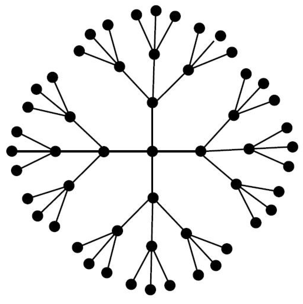
4.1. Monocentric Homogeneous Dendrimer Graph

A monocentric dendrimer $D(t,r)$ is a tree with two additional parameters: the progressive degree t and the radius r. Every internal vertex of the tree has degree $t+1$. A monocentric dendrimer tree has one central vertex, and its radius r is the maximum distance from any pendent vertex to the central one. If all pendent vertices are at a distance r from the central vertex, then the monocentric dendrimer is called homogeneous.For more details, please see [37,38]. Figure 1 is an example for a monocentric homogeneous dendrimer with $t=3$ and $r=3$.

To parameters t and r, we have the order $n=1+\frac{(t+1)(t^r-1)}{t-1}$, and $m=n-1$, $\Delta =t+1$, $\delta =1$. Let $t=3$, we change the value of parameter r to compute the degree-based network entropy $NE\left(D\right(3,r\left)\right)$ and bounds $U_{NE}$, $L_{NE}$. The results are listed in

Table 1. Some values of the degree-based network entropy and bounds for $D(3,r).$

r	$\mathbf{NE}\left(\mathbf{D}\right(\mathbf{3},\mathbf{r}\left)\right)$	${\mathit{U}}_{\mathit{NE}}$	${\mathit{L}}_{\mathit{NE}}$
1	2.0000	2.1738	1.8734
2	3.7500	4.0780	3.7496
3	5.3928	5.7260	5.3911
4	6.9969	7.3304	6.9936
5	8.5883	8.9217	8.5843
6	10.1754	10.5087	10.1711
7	11.7610	12.0944	11.7567
8	13.3462	13.6796	13.3419
9	14.9313	15.2646	14.9269
10	16.5163	16.8496	16.5119
20	32.3659	32.6993	32.3615
30	48.2155	48.5489	48.2112
40	64.0652	64.3985	64.0608
50	79.9148	80.2481	79.9104
60	95.7644	96.0978	95.7600
70	111.6140	111.9474	111.6097
80	127.4637	127.7970	127.4593
90	143.3133	143.6466	143.3089
100	159.1629	159.4963	159.1585

.

In Table 1, we can see that the value of degree-based network entropy $NE\left(G\right)$ corresponds to the scale of the graph. The larger the order and size are, the bigger the degree-based network entropy is. This means that the corresponding graph is more complex in the structural information. Furthermore the bounds we obtained are very close to the real value of entropy. Relatively speaking, the entropy is nearer to the lower bound $L_{NE}$ than to the upper bound $U_{NE}$. Compared with the list for them in Table 3 in [33], we also find the new lower bound is better.

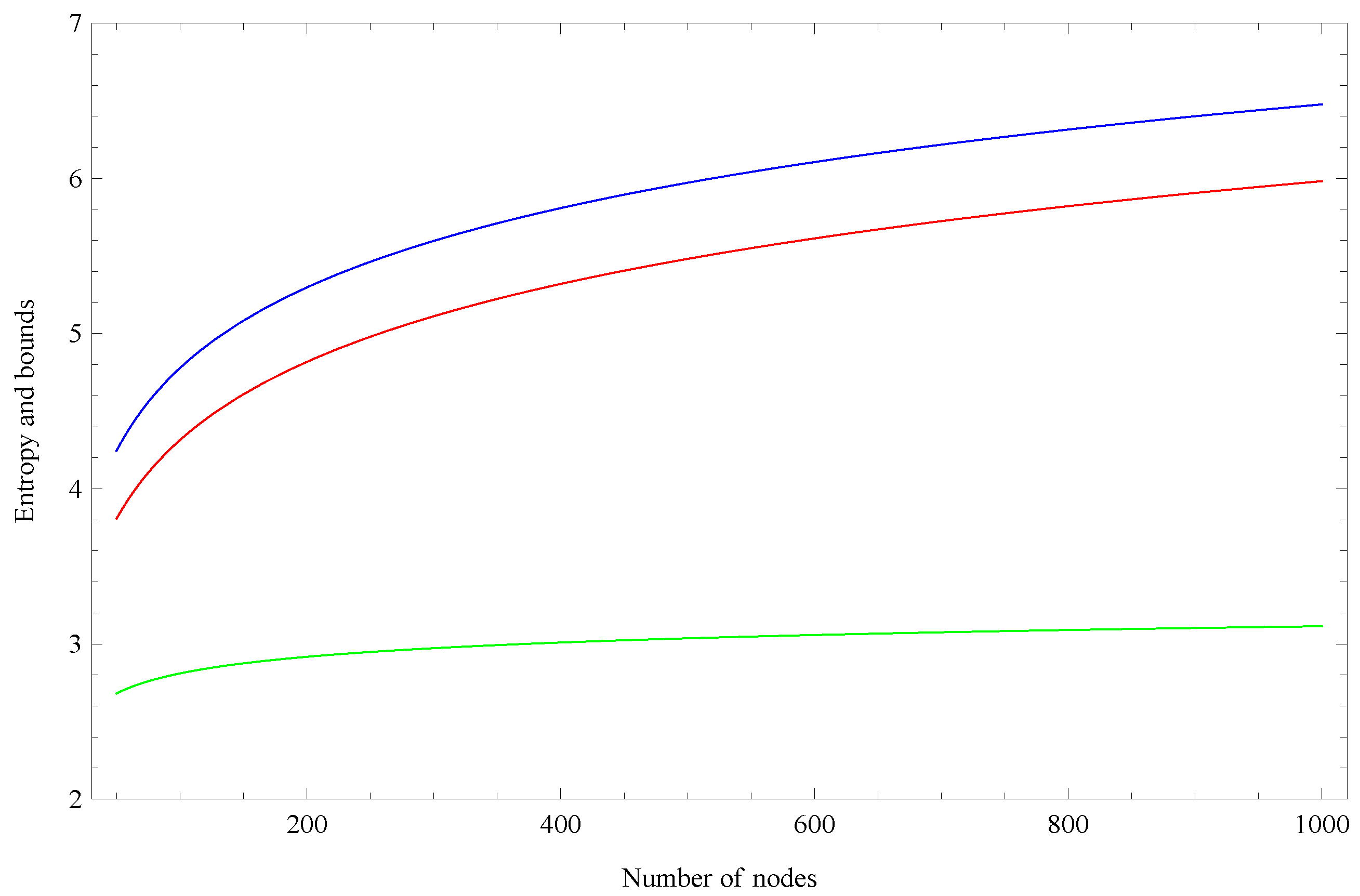
4.2. Star Graph

A star graph $S_n$ is a tree of order n with one internal vertex and $n-1$ pendent vertices. So in $S_n$ one internal vertex has degree $n-1$, while all others (if any) have degree 1. Moreover, $m=n-1$, $\Delta =n-1$, $\delta =1$.

In Figure 2, the values of $NE$(red), $U_{NE}$(blue) and $L_{NE}$(green) with $n\in [50,1000]$ are shown. We can see that the value of degree-based network entropy $NE\left(S_n\right)$ is increasing with the order n of the star graph $S_n$. The result also demonstrates that the degree-based network entropy corresponds to the scale of the same type graph. Furthermore, the growth of the lower bound $L_{NE}$ is flat, but the growths of the upper bound $U_{NE}$ and the entropy are steep. The entropy is nearer to the upper bound $U_{NE}$ than to the lower bound $L_{NE}$. Maybe the upper bound $U_{NE}$ contains more information because its change trend is consistent with that of the entropy.

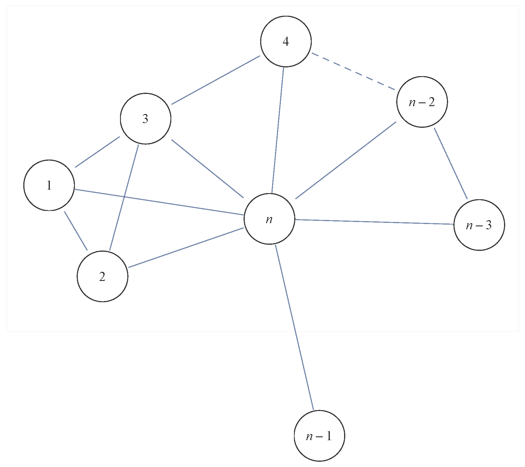
4.3. A Special Computer Network

Next we consider the following practical example, inspired from computer networks. We have a network with n nodes: a gateway (node n), a storage server connected only to the gateway (node $n-1$), and $n-2$ computers connected with the gateway and possible directly connected. Figure 3 highlights this model.

In this model, we can confirm that two nodes have fixed degree values: The degree of node n is $n-1$, and the degree of node $n-1$ is 1. For given n, the possible number of edges is

$$n-1\le m\le \frac{(n-1)(n-2)}{2}+1.$$

(14)

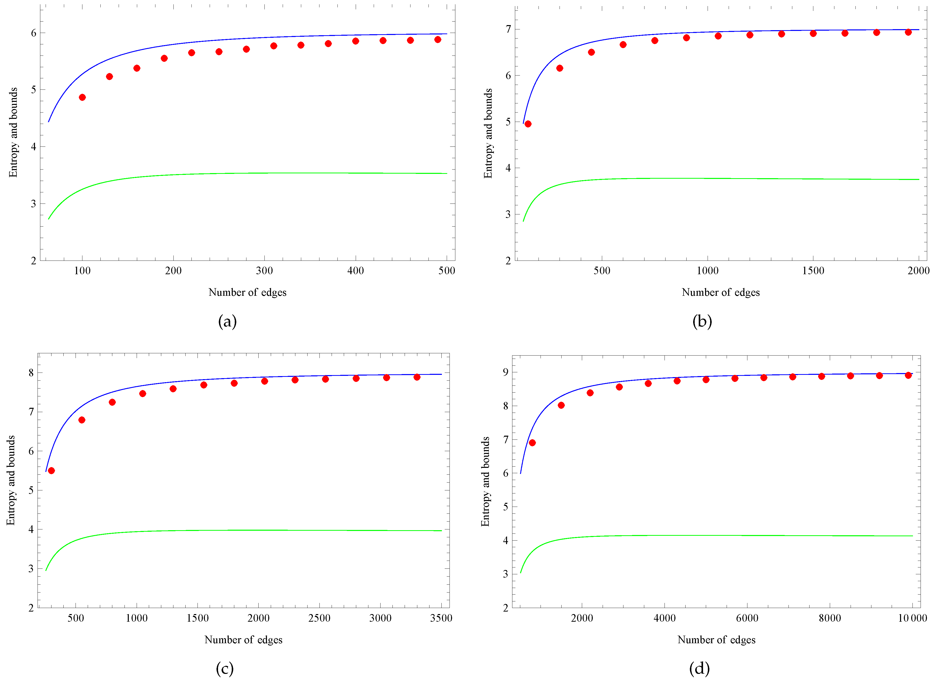
We let the values of n be $64,128,256,512$ respectively, and calculate the $NE$, $U_{NE}$ and $L_{NE}$ with different m in the range (14).

The results are graphically represented in Figure 4. The red dots indicate the values of degree-based network entropy in simulated networks. The blue lines indicate the upper bounds $U_{NE}$. The green lines indicate the lower bounds $L_{NE}$. We can see the degree-based network entropy $NE$ is increasing with the scale of order n and size m. As the size m increasing, the growth trend of the entropy becomes progressively flat. The entropy almost stabilizes after the drastic growth of size m in the beginning. Furthermore, the entropy is very close to the upper bound $U_{NE}$, especially when m and n are large enough (see the right half part of every sub-figure). In addition, we find that the computer network is comparable to the star graph by the change trends of $NE$, $U_{NE}$ and $L_{NE}$. Maybe they have some similar properties such as strong centrality, short average distance, weak robustness and so on. The node n in the computer network is analogous to the internal vertex in the star graph. But the computer network contains more structural information because the corresponding entropy is closer to the upper bound in comparison with star graph. The difference indicates that real networks are more complex than the regular star-graph networks.

Above all, we can analyze and obtain the structural complexity for the computer network by considering only two stable nodes without the connections of other nodes. The results can bring very important impact in overlays construction for computer networks.

5. Summary and Conclusions

In this paper, we studied the properties for degree-based network entropy $NE$. We proposed a new approach to analyze the entropy by determining its bounds. The new upper bound and lower bound are based on a new refinement of Jensen’s inequality. Moreover, they can estimate $NE$ only by using the order n, the size m, the maximum degree and minimum degree of a given network. We showed the numerical results which reflect the effects of $NE$ for special graphs such as monocentric homogeneous dendrimer graph and star graph. As an application to structural complexity analysis of a computer network modeled by a connected graph, we did the simulation for different numbers of nodes and edges. The bounds of degree-based network entropy can be also used to national security, internet networks, social networks, structural chemistry, ecological networks, computational systems biology, etc. They will play an important role in analyzing structural symmetry and asymmetry in real networks in the future.

References

- Shannon, C.E. A mathematical theory of communication. Bell Syst. Tech. J. 1948, 27, 379–423, 623–656. [Google Scholar] [CrossRef]
- Rashevsky, N. Life, information theory, and topology. Bull. Math. Biophys. 1955, 17, 229–235. [Google Scholar] [CrossRef]
- Mowshowitz, A. Entropy and the complexity of the graphs: I. An index of the relative complexity of a graph. Bull. Math. Biophys. 1968, 30, 175–204. [Google Scholar] [CrossRef] [PubMed]
- Solé, R.V.; Montoya, J.M. Complexity and fragility in ecological networks. Proc. R. Soc. Lond. B Biol. Sci. 2001, 268, 2039–2045. [Google Scholar] [CrossRef] [PubMed]
- Mehler, A.; Lücking, A.; Weiß, P. A network model of interpersonal alignment. Entropy 2010, 12, 1440–1483. [Google Scholar] [CrossRef]
- Ulanowicz, R.E. Quantitative methods for ecological network analysis. Comput. Biol. Chem. 2004, 28, 321–339. [Google Scholar] [CrossRef] [PubMed]
- Dehmer, M.; Barbarini, N.; Varmuza, K.; Graber, A. Novel topological descriptors for analyzing biological networks. BMC Struct. Biol. 2010, 10. [Google Scholar] [CrossRef] [PubMed]
- Dehmer, M.; Graber, A. The discrimination power of molecular identification numbers revisited. MATCH Commun. Math. Comput. Chem. 2013, 69, 785–794. [Google Scholar]
- Watts, D.J.; Strogatz, S.H. Collective dynamics of “small-world” networks. Nature 1998, 393, 440–442. [Google Scholar] [CrossRef] [PubMed]
- Barabási, A.L. Scale-free networks: A decade and beyond. Science 2009, 325, 412–413. [Google Scholar] [CrossRef] [PubMed]
- Cohen, R.; Havlin, S. Scale-free networks are ultrasmall. Phys. Rev. Lett. 2003, 90, 058701. [Google Scholar] [CrossRef] [PubMed]
- Newman, M.E.J. The structure and function of complex networks. SIAM Rev. 2003, 45, 167–256. [Google Scholar] [CrossRef]
- Boccaletti, S.; Latora, V.; Moreno, Y.; Chavez, M.; Hwang, D.-U. Complex networks: Structure and dynamics. Phys. Rep. 2006, 424, 175–308. [Google Scholar] [CrossRef]
- Song, C.; Havlin, S.; Makse, H.A. Self-similarity of complex networks. Nature. 2005, 433, 392–395. [Google Scholar] [CrossRef] [PubMed]
- Wei, D.; Wei, B.; Hu, Y.; Zhang, H.; Deng, Y. A new information dimension of complex networks. Phys. Lett. A. 2014, 378, 1091–1094. [Google Scholar] [CrossRef]
- Dehmer, M. Information-theoretic concepts for the analysis of complex networks. Appl. Artif. Intell. 2008, 22, 684–706. [Google Scholar] [CrossRef]
- Dehmer, M. A novel method for measuring the structural information content of networks. Cybernet. Syst. 2008, 39, 825–843. [Google Scholar] [CrossRef]
- Dehmer, M.; Borgert, S.; Emmert-Streib, F. Entropy bounds for molecular hierarchical networks. PLoS ONE 2008, 3, e3079. [Google Scholar] [CrossRef] [PubMed]
- Dehmer, M.; Emmert-Streib, F. Structural information content of networks: Graph entropy based on local vertex functionals. Comput. Biol. Chem. 2008, 32, 131–138. [Google Scholar] [CrossRef] [PubMed]
- Dehmer, M.; Emmert-Streib, F. Towards network complexity. Volume 4 of Lecture Notes of the Institute for Computer Sciences, Social Informatics and Telecommunications Engineering. In Complex Sciences; Zhou, J., Ed.; Springer: Berlin, Germany; Heidelberg, Germany, 2009; pp. 707–714. [Google Scholar]
- Bianconi, G. The entropy of randomized network ensembles. EPL Europhys. Lett. 2008, 81, 28005. [Google Scholar] [CrossRef]
- Xiao, Y.H.; Wu, W.T.; Wang, H.; Xiong, M.; Wang, W. Symmetry-based structure entropy of complex networks. Physica A 2008, 387, 2611–2619. [Google Scholar] [CrossRef]
- Anand, K.; Bianconi, G. Entropy measures for networks: Toward an information theory of complex topologies. Phys. Rev. E 2009, 80, 045102. [Google Scholar] [CrossRef] [PubMed]
- Cai, M.; Du, H.F.; Ren, Y.K.; Marcus, W. A new network structure entropy based node difference and edge difference. Acta. Phys. Sin. 2011, 60, 110513. [Google Scholar]
- Popescu, M.A.; Slusanschi, E.; Iancu, V.; Pop, F. A new bound in information theory. In Proceedings of the RoEduNet Conference 13th Edition: Networking in Education and Research Joint Event RENAM 8th Conference, Chisinau, Moldova, 11–13 September 2014; pp. 1–3.
- Garrido, A. Symmetry in Complex Networks. Symmetry 2011, 3, 1–15. [Google Scholar] [CrossRef]
- Dehmer, M. Information Theory of Networks. Symmetry 2011, 3, 767–779. [Google Scholar] [CrossRef]
- Mowshowitz, A.; Dehmer, M. Entropy and the complexity of graphs revisited. Entropy 2012, 14, 559–570. [Google Scholar] [CrossRef]
- Tan, Y.J.; Wu, J. Network structure entropy and its application to scale-free networks. Syst. Eng. Theory Pract. 2004, 6, 1–3. [Google Scholar]
- Cao, S.; Dehmer, M.; Shi, Y. Extremality of degree-based graph entropies. Inform. Sci. 2014, 278, 22–33. [Google Scholar] [CrossRef]
- Cao, S.; Dehmer, M. Degree-based entropies of networks revisited. Appl. Math. Comput. 2015, 261, 141–147. [Google Scholar] [CrossRef]
- Chen, Z.; Dehmer, M.; Shi, Y. Bounds for degree-based network entropies. Appl. Math. Comput. 2015, 265, 983–993. [Google Scholar] [CrossRef]
- Lu, G.; Li, B.; Wang, L. Some new properties for degree-based graph entropies. Entropy 2015, 17, 8217–8227. [Google Scholar] [CrossRef]
- Cover, T.M.; Thomas, J.A. Elements of Information Theory, 2nd ed.; Wiley & Sons: New York, NY, USA, 2006. [Google Scholar]
- Simic, S. Best possible global bounds for Jensen’s inequality. Appl. Math. Comput. 2009, 215, 2224–2228. [Google Scholar] [CrossRef]
- Simic, S. Jensen’s inequality and new entropy bounds. Appl. Math. Lett. 2009, 22, 1262–1265. [Google Scholar] [CrossRef]
- Chen, Z.; Dehmer, M.; Emmert-Streib, F.; Shi, Y. Entropy bounds for dendrimers. Appl. Math. Comput. 2014, 242, 462–472. [Google Scholar] [CrossRef]
- Chen, Z.; Dehmer, M.; Emmert-Streib, F.; Shi, Y. Entropy of Weighted Graphs with Randić Weights. Entropy 2015, 17, 3710–3723. [Google Scholar] [CrossRef]
© 2016 by the authors; licensee MDPI, Basel, Switzerland. This article is an open access article distributed under the terms and conditions of the Creative Commons by Attribution (CC-BY) license (http://creativecommons.org/licenses/by/4.0/).