
Cubature Formulas of Multivariate Polynomials Arising from Symmetric Orbit Functions


Abstract
:1. Introduction
2. Root Systems and Polynomials
2.1. Pertinent Properties of Root Systems and Weight Lattices
- The marks of the highest root .
- The Coxeter number of G.
- The Cartan matrix C and its determinant.
- The root lattice .
- The -dual lattice to Q,with the vectors given by
- The dual root lattice , where .
- The dual marks of the highest dual root . The marks and the dual marks are summarized in Table 1 in [7]. The highest dual root η satisfies for all
- The -dual weight lattice towith the vectors given by For the following notation is used,
- The partial ordering on P is given: for it holds that if and only if with for all .
- The half of the sum of the positive roots
- The cone of positive weights and the cone of strictly positive weights
- n reflections , in -dimensional “mirrors” orthogonal to simple roots intersecting at the origin denoted by
2.2. Affine Weyl Groups
2.3. Orbit Functions
3. Cubature Formulas
3.1. The X-Transform
3.2. The Cubature Formula
4. Cubature Formulas of Rank Two
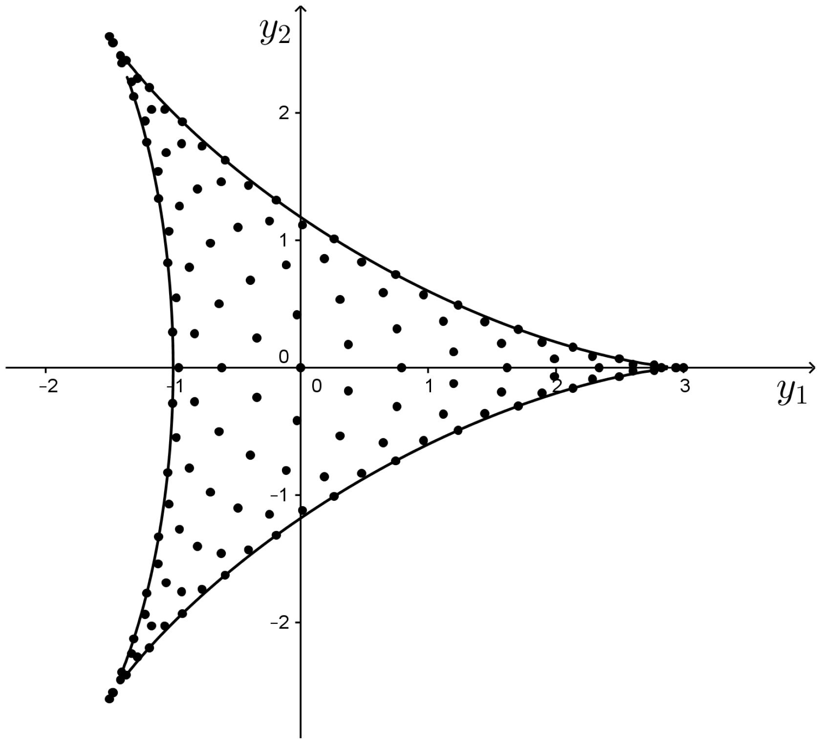
4.1. The Case
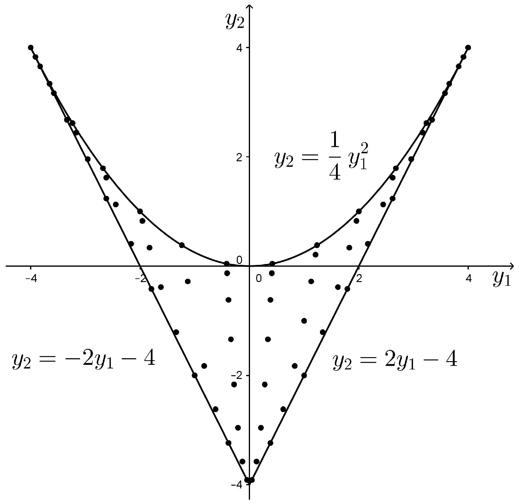
4.2. The Case
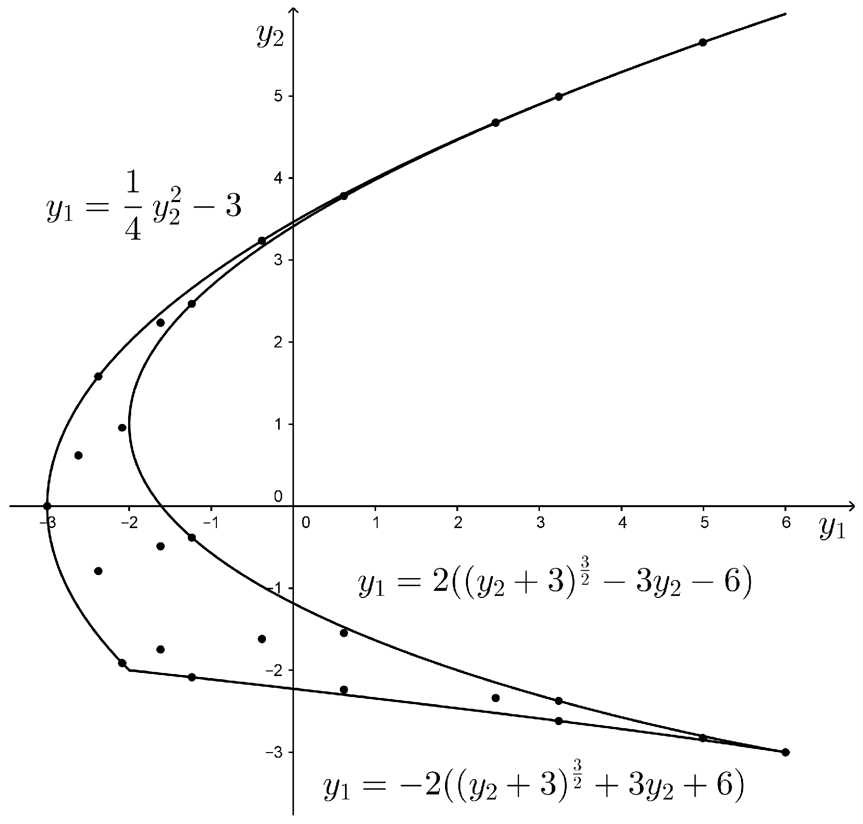
4.3. The Case
5. Polynomial Approximations
5.1. The Optimal Polynomial Approximation
5.2. The Cubature Polynomial Approximation
6. Conclusions
- Due to the generality of the present construction of the cubature formulas, some of the cases presented in this paper appeared already in the literature. The case is closely related to two-variable analogues of Jacobi polynomials on Steiner’s hypocycloid [26]; the case is related to two-variable analogues of Jacobi polynomials on a domain bounded by two lines and a parabola [26,27,28] and the corresponding Gaussian cubature formulas induced by these polynomials are studied for example in [10]. The case and its cubature formulas are detailed in [25].
- The Chebyshev polynomials of the first kind induce the cubature formula of the maximal efficiency—Gauss-Chebyshev quadrature [5,29]. The nodes of this formula are M roots of the Chebyshev polynomials of the first kind of degree M and it exactly evaluates a weighted integral for any polynomial of degree at most . The set of nodes of does not correspond to the set of roots of the Gauss-Chebyshev quadrature— of consists of points and includes two boundary points of the interval. Thus, the number of points exceeds by one the minimum number of nodes and the resulting cubature formula is not optimal. This phenomenon, already observed for the sequence in [9], generalizes to all cases of Weyl groups. Even though the developed formulas are slightly less efficient than the optimal ones, they contain points on the entire boundary of —this might be useful for some applications.
- The technique for construction of the cubature formulas in this article is based on discrete orthogonality of C-functions over the set . For the case the cosine transform corresponding to the discrete orthogonality of cosines is standardly known as discrete cosine transform of the type DCT-I [30]. The M roots of the Chebyshev polynomials of the first kind, which lead to the optimal cubature formula, enter the discrete orthogonality relations of the type DCT-II. This indicates that the discrete orthogonality relations of C-functions, which generalize the transforms of the type DCT-II, DCT-III and DCT-IV for admissible cases of Weyl groups [31], might lead to cubature formulas of higher efficiency.
- The weaker version of the polynomial approximation (60) assigns to any complex function a polynomial functional series . Existence of conditions for convergence of these functional series together with an estimate of the approximation error poses an open problem.
- The Clenshaw-Curtis method for deriving cubature formulas is based on expressing a given function into a series of the corresponding set of orthogonal polynomials and then integrating the series term by term [32,33]. The coefficients in the series are calculated using discrete orthogonality properties. The comparison of the resulting cubature formulas by the Clenshaw-Curtis technique and the method used in the present paper and in [1,2] deserves further study.
- The polynomials of the orbit functions used in the present paper and in [1,2] to derive the cubature formulas are directly related to the Jacobi polynomials associated to root systems as well as to the Macdonald polynomials. The discrete orthogonality of the Macdonald polynomials with unitary parameters, achieved in [34], opens a possibility of an extension of the current cubature formulas to the corresponding subset of the Macdonald polynomials.
Acknowledgments
Author Contributions
Conflicts of Interest
References
- Moody, R.V.; Motlochová, L.; Patera, J. Gaussian cubature arising from hybrid characters of simple Lie groups. J. Fourier Anal. Appl. 2014, 20, 1257–1290. [Google Scholar] [CrossRef]
- Moody, R.V.; Patera, J. Cubature formulae for orthogonal polynomials in terms of elements of finite order of compact simple Lie groups. Adv. Appl. Math. 2011, 47, 509–535. [Google Scholar]
- Bourbaki, N. Groupes et algèbres de Lie. Chapitres IV, V, VI, 1st ed.; Hermann: Paris, France, 1968. [Google Scholar]
- Klimyk, A.U.; Patera, J. Orbit functions. SIGMA 2014, 2, 60. [Google Scholar]
- Rivlin, T.J. The Chebyshev Polynomials; Wiley: New York, NY, USA, 1974. [Google Scholar]
- Moody, R.V.; Patera, J. Orthogonality within the families of C-, S-, and E-functions of any compact semisimple Lie group. SIGMA 2006, 2, 14. [Google Scholar] [CrossRef]
- Hrivnák, J.; Patera, J. On discretization of tori of compact simple Lie groups. J. Phys. A Math. Theor. 2009, 42, 385208. [Google Scholar]
- Cools, R. An encyclopaedia of cubature formulas. J. Complex. 2003, 19, 445–453. [Google Scholar]
- Li, H.; Xu, Y. Discrete Fourier analysis on fundamental domain and simplex of Ad lattice in d-variables. J. Fourier Anal. Appl. 2010, 16, 383–433. [Google Scholar]
- Schmid, H.J.; Xu, Y. On bivariate Gaussian cubature formulae. Proc. Am. Math. Soc. 1994, 122, 833–841. [Google Scholar]
- Caliari, M.; de Marchi, S.; Vianello, M. Hyperinterpolation in the cube. Comput. Math. Appl. 2008, 55, 2490–2497. [Google Scholar]
- Crivellini, A.; D’Alessandro, V.; Bassi, F. High-order discontinuous Galerkin solutions of three-dimensional incompressible RANS equations. Comput. Fluids 2013, 81, 122–133. [Google Scholar]
- Çapoğlu, İ.R.; Taflove, A.; Backman, V. Computation of tightly-focused laser beams in the FDTD method. Optics Express 2013, 21, 87–101. [Google Scholar]
- Xu, J.; Chen, J.; Li, J. Probability density evolution analysis of engineering structures via cubature points. Comput. Mech. 2012, 50, 135–156. [Google Scholar]
- Young, J.C.; Gedney, S.D.; Adams, R.J. Quasi-mixed-order prism basis functions for Nyström-based volume integral equations. IEEE Trans. Magn. 2012, 48, 2560–2566. [Google Scholar]
- Chernyshenko, D.; Fangohr, H. Computing the demagnetizing tensor for finite difference micromagnetic simulations via numerical integration. J. Magn. Magn. Mat. 2015, 381, 440–445. [Google Scholar]
- Sfevanovic, I.; Merli, F.; Crespo-Valero, P.; Simon, W.; Holzwarth, S.; Mattes, M.; Mosig, J.R. Integral equation modeling of waveguide-fed planar antennas. IEEE Antenn. Propag. M. 2009, 51, 82–92. [Google Scholar]
- Tasinkevych, M.; Silvestre, N.M.; Telo da Gama, M.M. Liquid crystal boojum-colloids. New J. Phys. 2012, 14, 073030. [Google Scholar]
- Lauvergnata, D.; Nauts, A. Quantum dynamics with sparse grids: A combination of Smolyak scheme and cubature. Application to methanol in full dimensionality. Spectrochim. Acta A 2014, 119, 18–25. [Google Scholar]
- Bjorner, A.; Brenti, F. Combinatorics of Coxeter Groups; Springer: New York, NY, USA, 2005. [Google Scholar]
- Humphreys, J.E. Reflection groups and Coxeter Groups; Cambridge University Press: Cambridge, UK, 1990. [Google Scholar]
- Vinberg, E.B.; Onishchik, A.L. Lie Groups and Lie Algebras; Springer: New York, NY, USA, 1994. [Google Scholar]
- Klimyk, A.U.; Patera, J. Antisymmetric orbit functions. SIGMA 2007, 3, 83. [Google Scholar]
- Li, H.; Sun, J.; Xu, Y. Discrete Fourier analysis, cubature and interpolation on a hexagon and a triangle. SIAM J. Numer. Anal. SIAM J. Numer. Anal. 2008, 46, 1653–1681. [Google Scholar]
- Li, H.; Sun, J.; Xu, Y. Discrete Fourier Analysis and Chebyshev Polynomials with G2 Group. SIGMA 2012, 8, 29. [Google Scholar]
- Koornwinder, T.H. Two-Variable Analogues of the Classical Orthogonal Polynomials. Theory and Application of Special Functions; Academic Press: New York, NY, USA, 1975; pp. 435–495. [Google Scholar]
- Koornwinder, T.H. Orthogonal polynomials in two variables which are eigenfunctions of two algebraically independent partial differential operators I–II. Kon. Ned. Akad. Wet. Ser. A 1974, 77, 46–66. [Google Scholar]
- Koornwinder, T.H. Orthogonal polynomials in two variables which are eigenfunctions of two algebraically independent partial differential operators III–IV. Indag. Math. 1974, 36, 357–381. [Google Scholar]
- Handscomb, D.C.; Mason, J.C. Chebyshev Polynomials; CRC: Boca Raton, FL, USA, 2003. [Google Scholar]
- Britanak, V.; Yip, P.; Rao, K. Discrete Cosine and Sine Transforms. General Properties, Fast Algorithms and Integer Approximations; Academic Press: Amsterdam, The Netherlands, 2007. [Google Scholar]
- Czyżycki, T.; Hrivnák, J. Generalized discrete orbit function transforms of affine Weyl groups. J. Math. Phys. 2014, 55, 113508. [Google Scholar]
- Clenshaw, C.W.; Curtis, A.R. A method for numerical integration on an automatic computer. Numer. Math. 1960, 2, 197–205. [Google Scholar]
- Sloan, I.H.; Smith, W.E. Product-integration with the Clenshaw-Curtis and related points. Numer. Math. 1978, 30, 415–428. [Google Scholar]
- Van Diejen, J.F.; Emsiz, E. Orthogonality of Macdonald polynomials with unitary parameters. Math. Z. 2014, 276, 517–542. [Google Scholar]


| 6 | 8 | 12 | |
| 2 | 2 | 2 | |
| 2 | 2 | 2 | |
| 1 | 1 | 1 |
| 1 | 1 | 1 | |
| 1 | 2 | 3 | |
| 1 | 1 | 2 | |
| 3 | 4 | 6 | |
| 3 | 4 | 6 | |
| 3 | 4 | 6 | |
| 6 | 8 | 12 |
| M | 10 | 20 | 30 | 50 | 100 | Exact Value |
|---|---|---|---|---|---|---|
| 66 | 231 | 496 | 1326 | 5151 | - | |
| 36 | 121 | 256 | 676 | 2601 | - | |
| 14 | 44 | 91 | 234 | 884 | - |
| M | 10 | 20 | 30 |
|---|---|---|---|
© 2016 by the authors; licensee MDPI, Basel, Switzerland. This article is an open access article distributed under the terms and conditions of the Creative Commons Attribution (CC-BY) license (http://creativecommons.org/licenses/by/4.0/).
Share and Cite
Hrivnák, J.; Motlochová, L.; Patera, J. Cubature Formulas of Multivariate Polynomials Arising from Symmetric Orbit Functions. Symmetry 2016, 8, 63. https://doi.org/10.3390/sym8070063
Hrivnák J, Motlochová L, Patera J. Cubature Formulas of Multivariate Polynomials Arising from Symmetric Orbit Functions. Symmetry. 2016; 8(7):63. https://doi.org/10.3390/sym8070063
Chicago/Turabian StyleHrivnák, Jiří, Lenka Motlochová, and Jiří Patera. 2016. "Cubature Formulas of Multivariate Polynomials Arising from Symmetric Orbit Functions" Symmetry 8, no. 7: 63. https://doi.org/10.3390/sym8070063