Relationship between Fractal Dimension and Spectral Scaling Decay Rate in Computer-Generated Fractals

Abstract

Two measures are commonly used to describe scale-invariant complexity in images: fractal dimension (D) and power spectrum decay rate (β). Although a relationship between these measures has been derived mathematically, empirical validation across measurements is lacking. Here, we determine the relationship between D and β for 1- and 2-dimensional fractals. We find that for 1-dimensional fractals, measurements of D and β obey the derived relationship. Similarly, in 2-dimensional fractals, measurements along any straight-line path across the fractal’s surface obey the mathematically derived relationship. However, the standard approach of vision researchers is to measure β of the surface after 2-dimensional Fourier decomposition rather than along a straight-line path. This surface technique provides measurements of β that do not obey the mathematically derived relationship with D. Instead, this method produces values of β that imply that the fractal’s surface is much smoother than the measurements along the straight lines indicate. To facilitate communication across disciplines, we provide empirically derived equations for relating each measure of β to D. Finally, we discuss implications for future research on topics including stress reduction and the perception of motion in the context of a generalized equation relating β to D.

1. Introduction

Researchers from diverse disciplines ranging from physics to psychology have converged on the question of how to quantify the scaling symmetry of natural objects. In one camp, fractals researchers describe objects such as clouds, coastlines, mountain ridgelines, and trees using a scale-invariant power law to measure the rate at which structure appears as the scale of measurement decreases [1,2,3,4,5,6], though debates continue regarding which power-laws, if any, best describe natural phenomena [7,8,9,10,11]. The following equation is a common example:

N ~ L^−D

(1)

where N is the extent to which the fractal fills space as measured at scale L [1,4]. The power law’s exponent D is called the fractal dimension.

Consider Figure 1a,b, which plots a fractal terrain in x, y, and z space, as a demonstration of how D relates to the object’s Euclidean dimension E. The topological dimension of this surface is E = 2 and it is embedded in a space of E = 3. Its fractal dimension, D_(Surface), lies in the range between these two Euclidean dimensions: 2 < D_(Surface) < 3. Taking a vertical slice through this terrain (i.e., taking its intersection with the xz or yz plane) creates a fractal “mountain” profile (see Figure 1c) quantified by D_{(Mountain Edge)} = D_(Surface) − 1. Similarly, taking a horizontal slice creates a fractal “coastline” (see Figure 1d) with D_{(Coastal Edge)} = D_{(Mountain Edge)}. To measure D_(Surface), mathematicians and natural scientists typically determine D_{(Mountain Edge)} or D_{(Coastal Edge)} (and then add 1) because the measurements involved are easier and faster to implement than for measurements of D_(Surface).

Vision researchers similarly use a power law to capture the scale-invariant properties of the fractal. However, they typically focus on the power spectrum decay rate (β) of the terrain’s intensity image [12,13,14,15,16,17,18,19,20,21]. This intensity image is generated by converting the terrain height into either grayscale variations (high is white, black is low) to create a grayscale map (see Figure 1b) or color variations to create a “heat map”. The following power law then characterizes the fractal structure in these maps and has, in particular, proved useful for quantifying the spectral scaling decay rate of grayscale images of natural scenes:

S_V(f) = 1/(cf^β)

(2)

where S_V(f) is the spectral density (power), f is the spatial frequency, and β and c are constants.

Voss [5] considered the Hurst exponent H, which by definition is related to D as follows:

D = E + 1 − H

(3)

where E is the Euclidean topological dimension. H and D lie in the following ranges: 0 < H < 1, E < D < E + 1. He then derived the relationship between H and β for a fractional Brownian function:

β = 2H + 1

(4)

where 1 < β < 3. Accordingly, Voss [5] stated that an approximation of the relationship for “the statistically self-affine fractional Brownian function V_H(x), with x in an E-dimensional Euclidian space, which has a fractal dimension D and spectral density S_V(f) ∝ 1/f^β, for the fluctuations along a straight line path in any direction in E-space” is provided by the equation

D = E + (3 − β)/2

(5)

However, through this definition, Voss [5] stipulates a different measure of β than that typically used by vision researchers. The definition specifies the measure of β be taken along the intersection of the fractal with a plane parallel to the z-axis—a mountain edge—and measuring the spectral decay of the 1-dimensional trace—a mountain profile. Thus, β in Equations (4) and (5) are what we will hereafter call β_{(Mountain Edge)}.

The relationship highlighted in Equation (5) between D and β_{(Mountain Edge)} has not been observed empirically for either 1-dimensional (E = 1, D ≤ 2) or 2-dimensional (E = 2, D ≤ 3) fractals. To experimentally discern this relationship, we use two methods for generating fractals—namely, midpoint displacement fractals (in which D serves as the input parameter) and fractal Fourier noise (in which β is the input). We find that, when measured along a straight-line path, the relationship described by Voss [5] holds for fractals with both E = 1 and 2. However, the relationship described by Voss [5] does not extend to the observed relationship between measurements of D and β when β is measured by the standard method of vision researchers (in a 2-dimensional Fourier space, which we will hereafter call β_(Surface)). A new equation that extends the relationship between D and β to multi-dimensional Fourier spaces has the potential to enhance discourse among mathematicians, who are experts in the geometry of fractals, physicists, who are experts in surfaces and textures, and vision scientists, who are experts in animals’ sensation and perception of geometric shapes, surfaces, and textures.

Further consideration of the relationship between D and β is both important and timely because new studies are being performed using fractals to investigate a variety of behaviors including aesthetics [22,23,24,25,26,27], navigation [28], object pareidolia (perceiving coherent forms in noise) [29,30], sensitivity [24], and associated neural mechanisms [31,32,33]. This is especially important in aesthetics research, where there have been claims of universality in preference for patterns of moderately low complexity [23,26,34,35,36,37]. To test this hypothesis, it is necessary to be able to translate the units of measurement of researchers who alternately use D [22,25,26,28,29,31,33,34,35,36,37,38,39,40], β [14,24,30,32,41,42,43,44,45,46], or, infrequently, both [23,27]. The crux of the problem, perhaps, is that D is a general parameter that quantifies complexity in a variety of patterns, whereas β is limited (at least in practice) in its ability to quantify some patterns’ complexity. For example, Fourier analysis is poorly suited to describe the complexity of patterns including strange attractors and some line fractals (e.g., dragon fractals and Koch snowflakes), which have been used by vision researchers to study aesthetics [25,31,34,35] and perceived complexity [47]. This provides a strong impetus to convert to D when forming general conclusions. Still, there is a great deal of utility in presenting fractal noise patterns that are defined in terms of β as visual stimuli, precisely because they mimic the statistics of natural scenes [12,13,15,16,17,18,19,20,21]. Here, we provide the basis for translation between the parameters D and β in a general equation that follows from empirical analysis of the relationships between measures of D and β.

2. Materials and Methods

Midpoint displacement and Fourier noise fractals were generated and analyzed in MATLAB version 2015b.

2.1. Midpoint Displacement Fractals

Sets of random midpoint displacement fractal lines (see Section 2.1.1) and images (see Section 2.1.2) were generated using an algorithm described by Fournier, Fussel, and Carpenter [2], which allowed us to specify D.

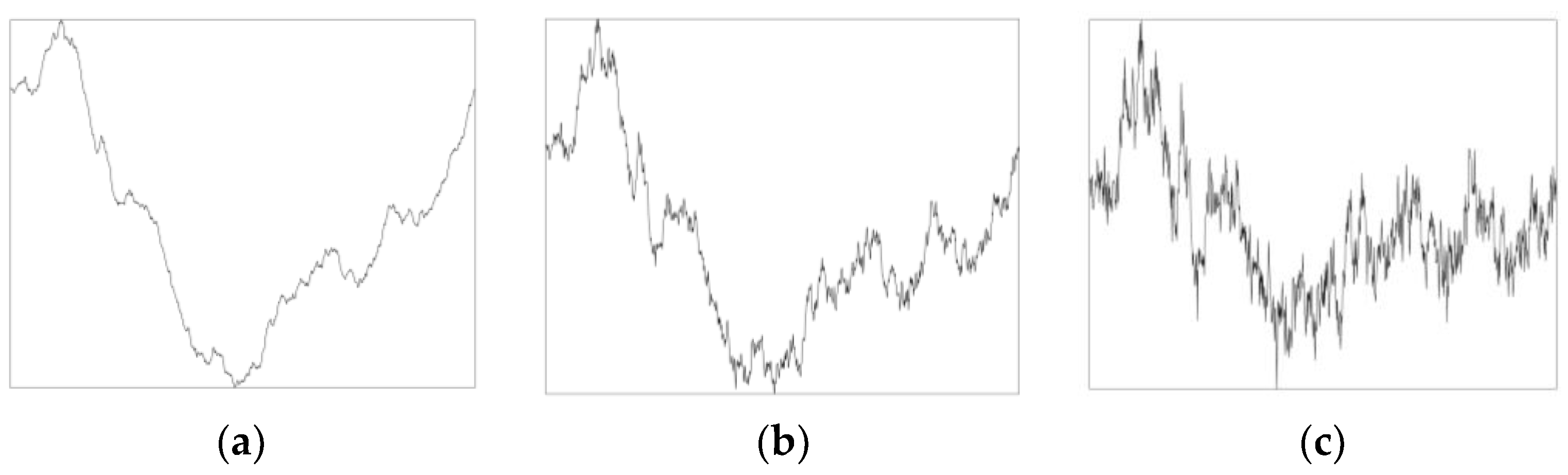
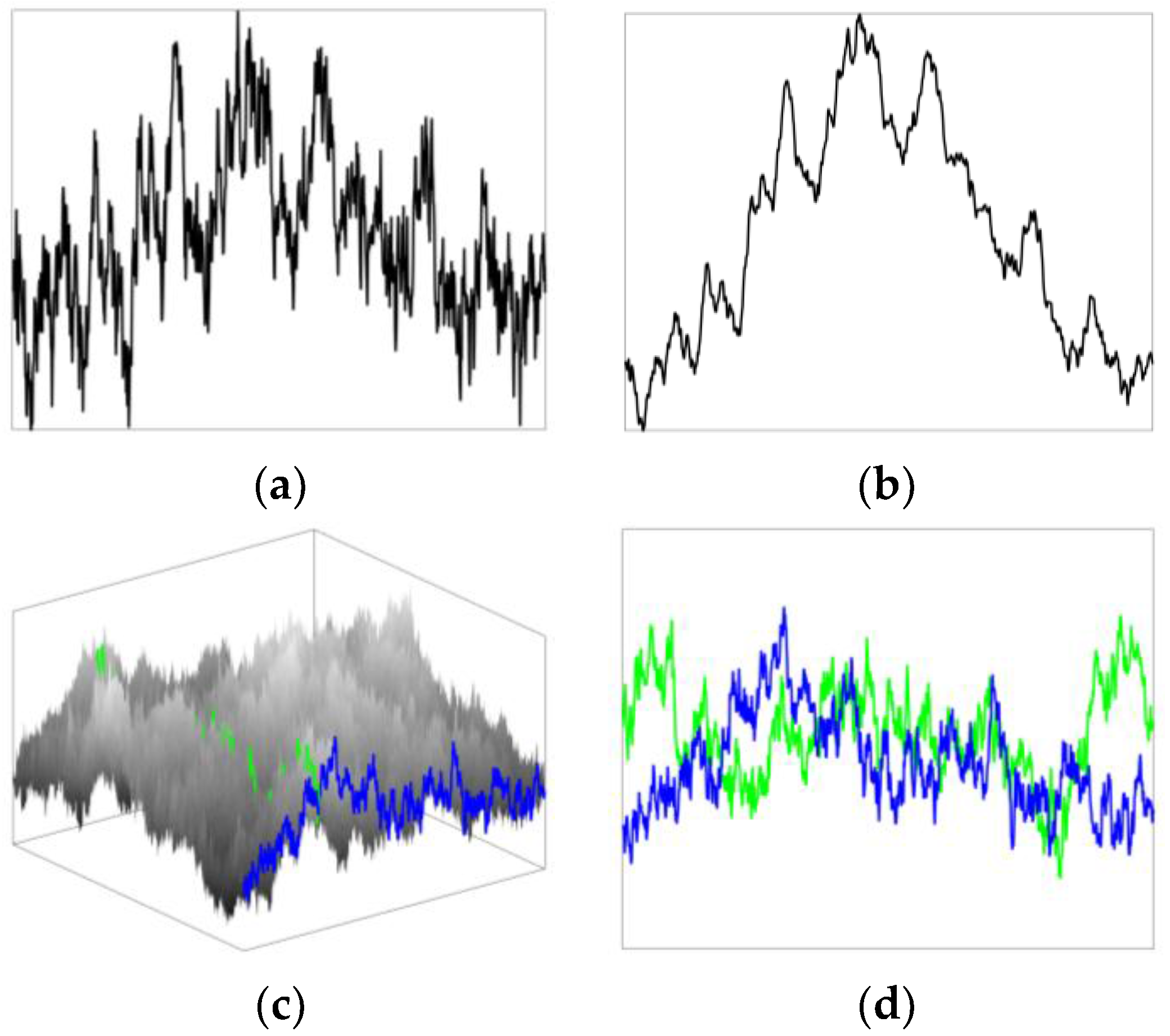
2.1.1. One-Dimensional Midpoint Displacement Fractals

To generate each 1-dimensional midpoint displacement fractal as a trace, a vertex, V, was added to the midpoint of an initial set of two endpoints and displaced vertically by a value randomly selected from a Gaussian distribution, with σ = 1, that was scaled by a factor of 2^{−2(3 − D)(R + 1)}, where D is the fractal dimension and R is the current level of recursion. This process is shown schematically for an exact midpoint displacement fractal that is not affected by random perturbations in Figure 2. As in the schematic, the scaling factor of the fractals generated for this study was held constant for each vertex at a given level of recursion, and changed with each level of recursion. The vertices at each recursion served as endpoints in the next level of recursion for R recursions in order to generate time-series data.

We retained the random values used for vertical displacement to generate sets of fractals that varied in D but retained the structure introduced at each level of recursion (see Figure 3).

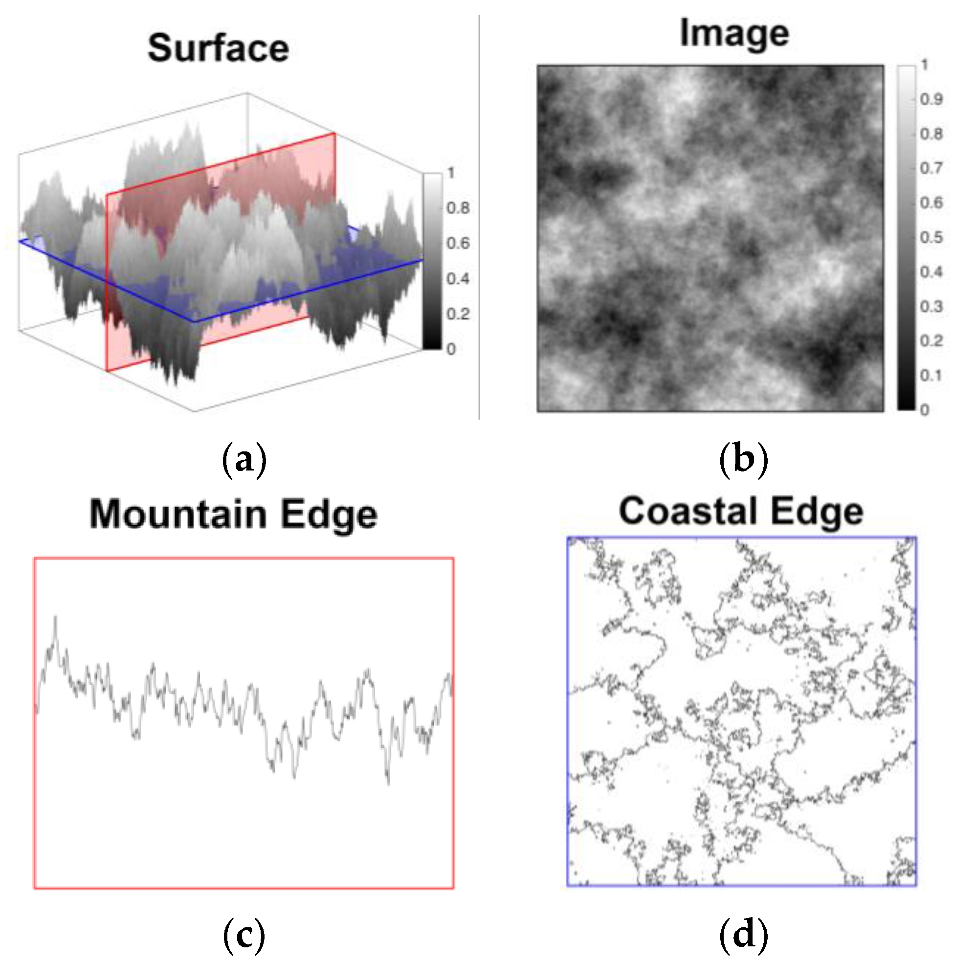
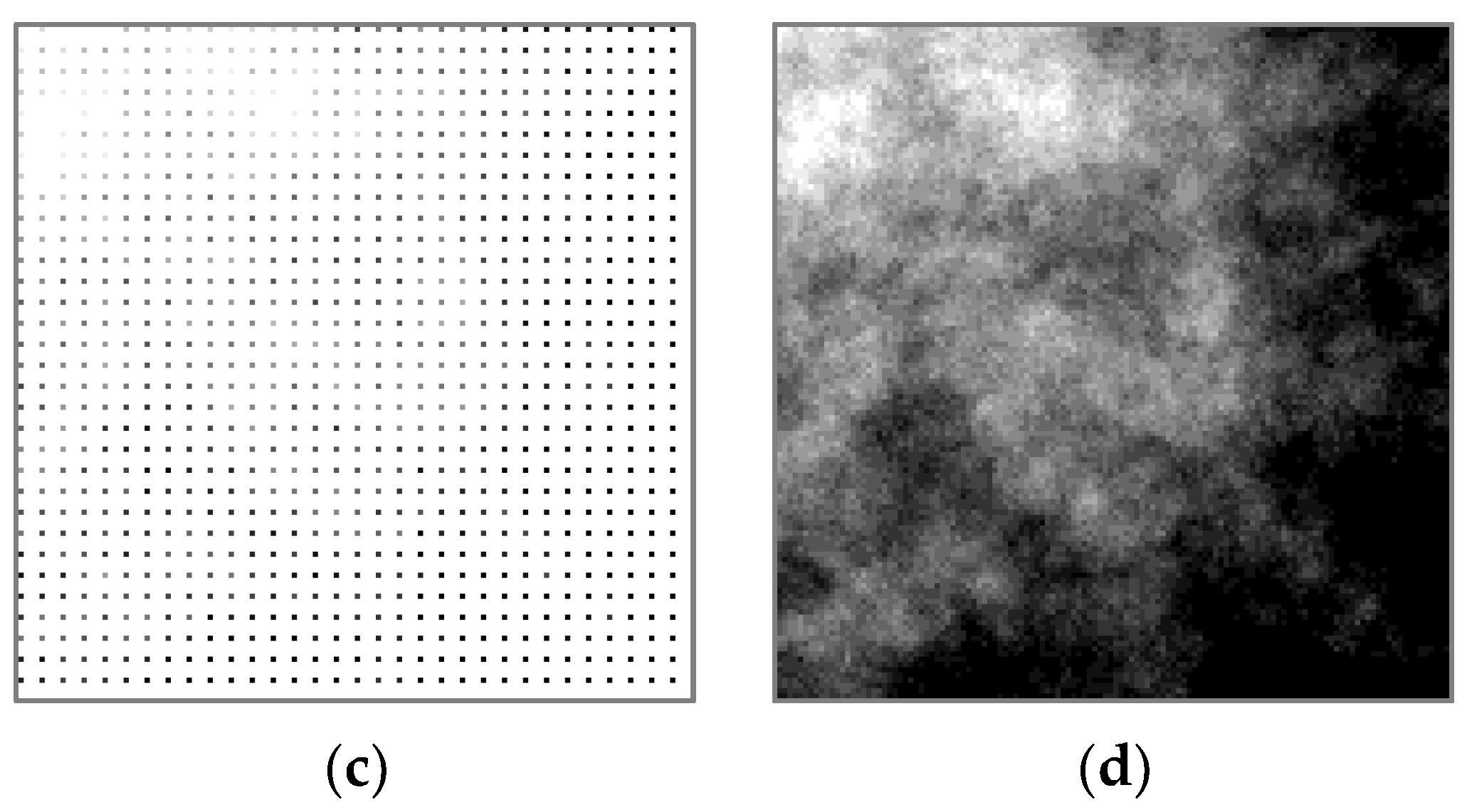
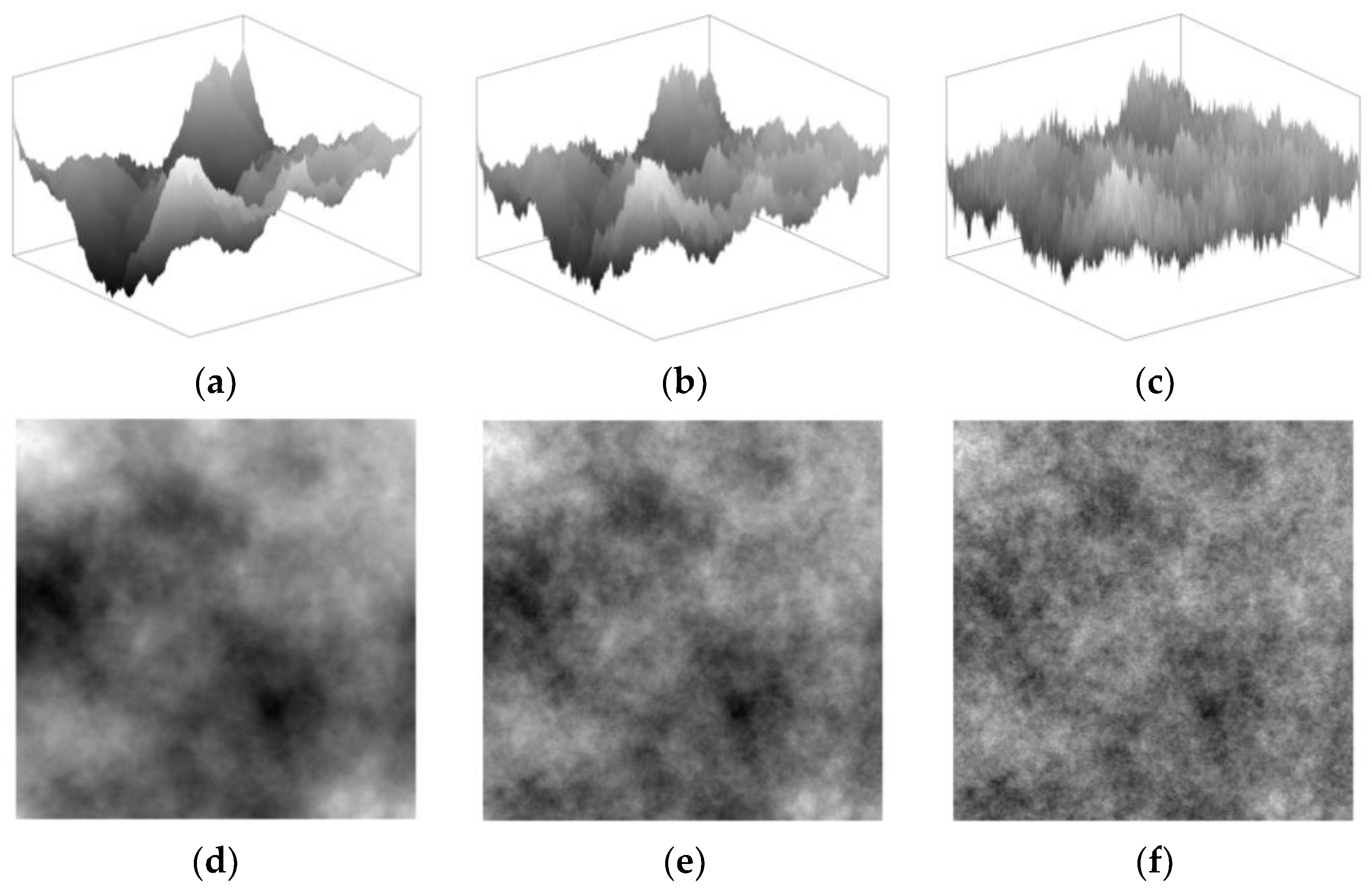
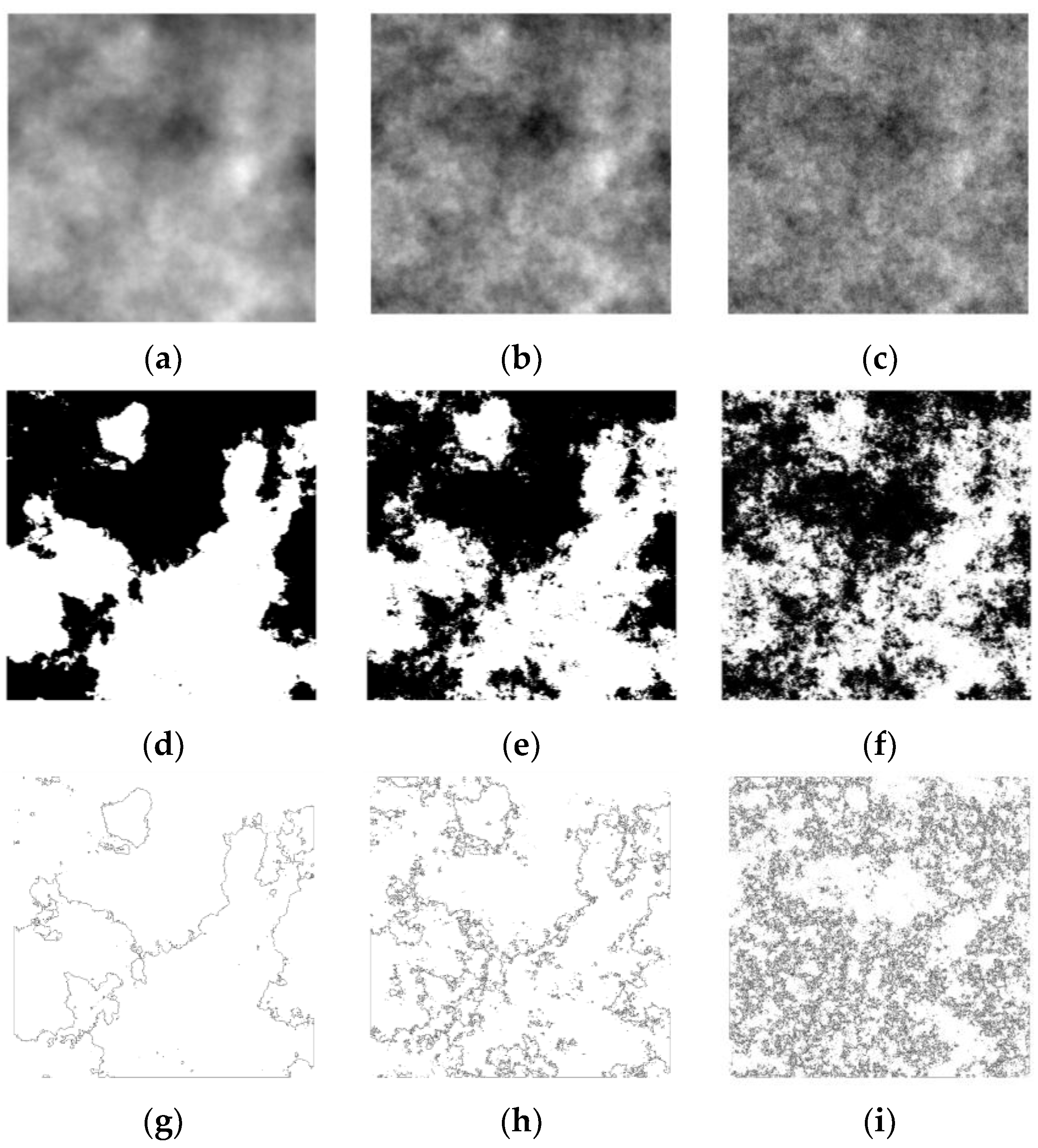
2.1.2. Two-Dimensional Midpoint Displacement Fractals

To generate each 2-dimensional midpoint displacement fractal as an image, a vertex, V, was added to the midpoint of an initial set of four edge points and displaced according to the generation rules described in Section 2.1.1 (see illustration of the generation process in Figure 4). The vertices at each recursion served as edges in the next level of recursion for n recursions in order to generate gray-scale intensity images.

We retained the random values used for vertical displacement to generate sets of fractal terrains that varied in D but retained consistent large-scale structures (see Figure 5).

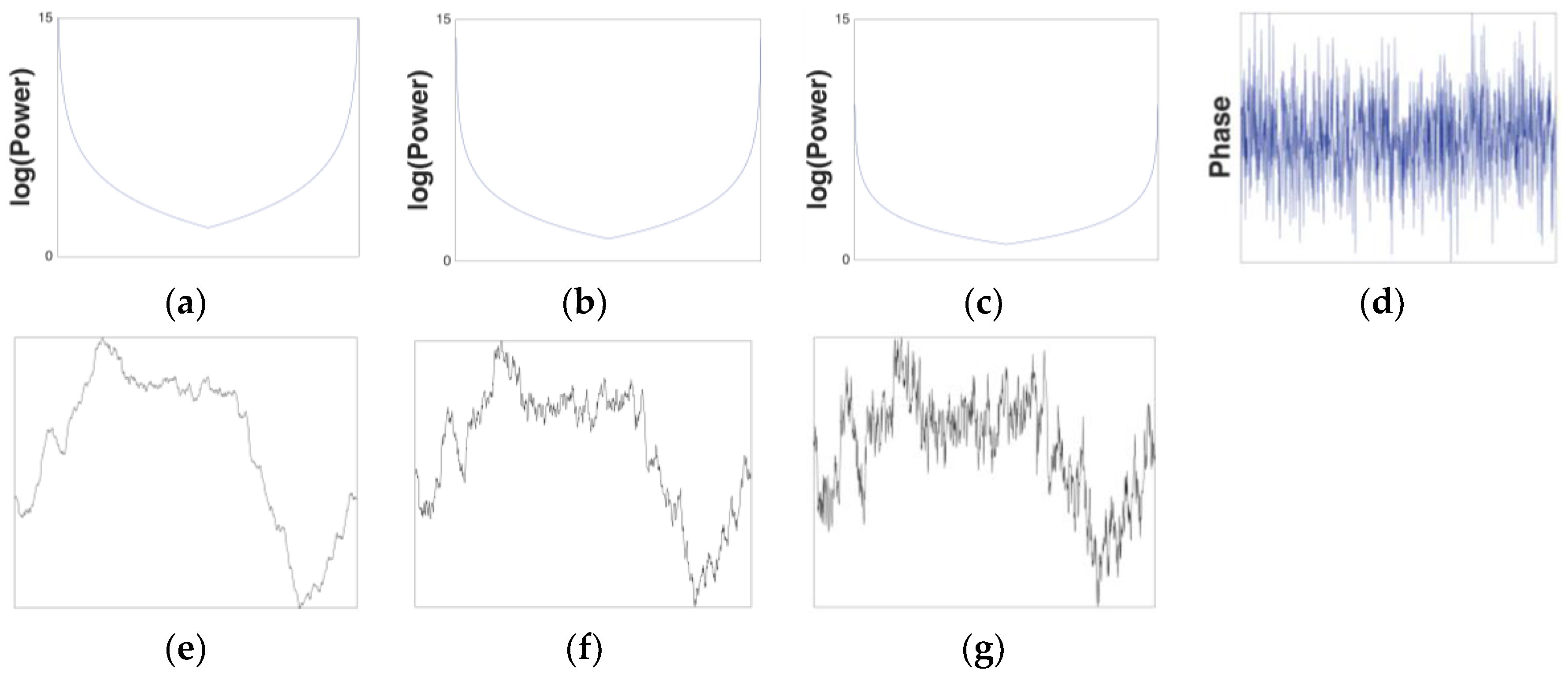
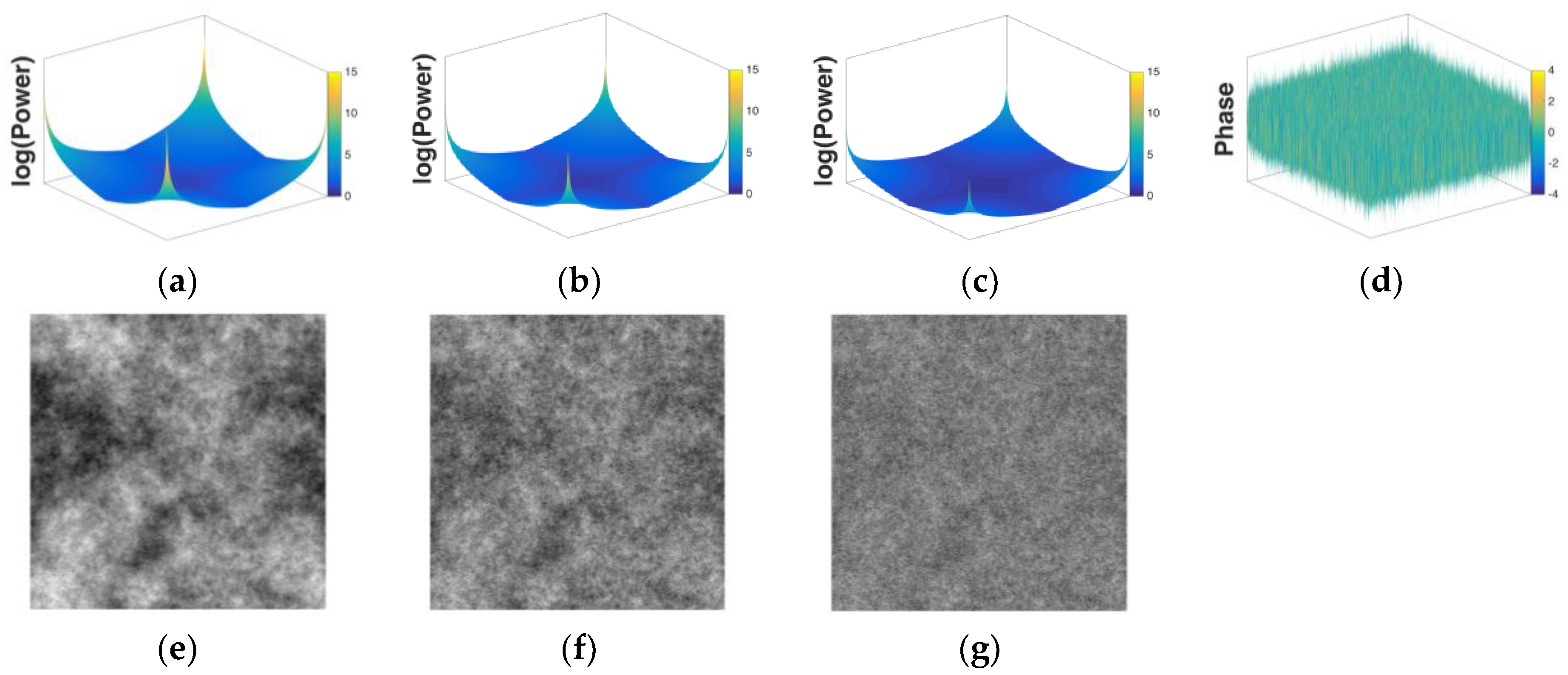
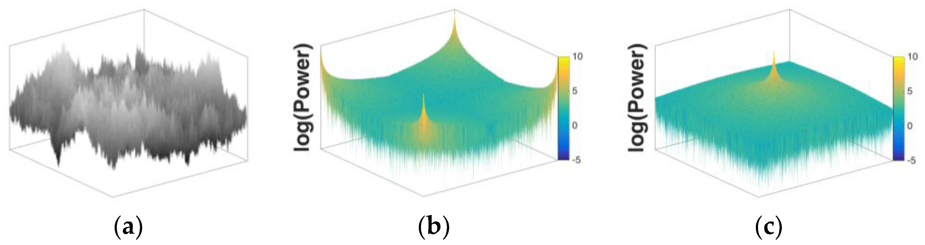
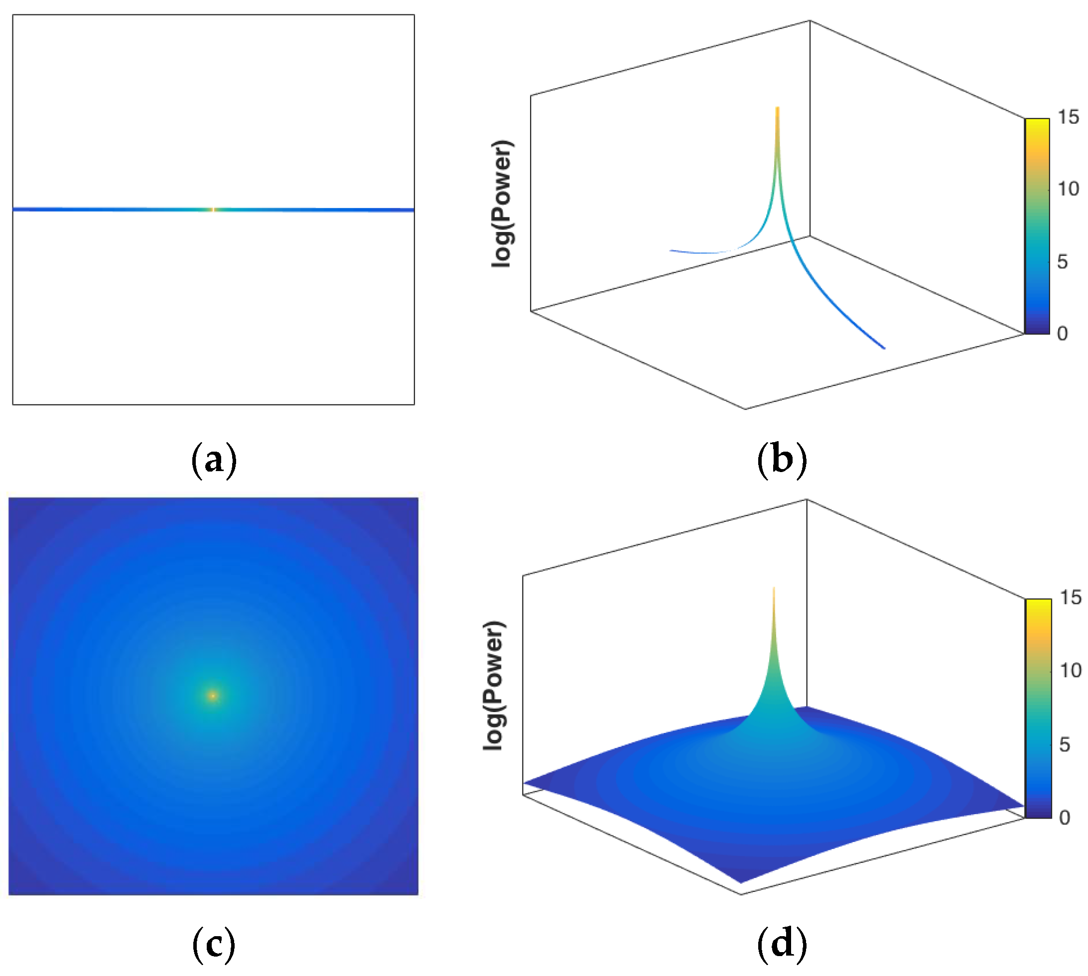
2.2. One- and Two-Dimensional Fractal Fourier Noise

Sets of fractal noise were generated using an algorithm described by Saupe [3], which allowed us to specify β.

For an image of size x by y pixels, an x by y amplitude matrix is created in which amplitude is specified for each spatial frequency by applying Equation (2). Each frequency is then assigned a phase specified by a phase matrix of size x by y, which consists of numbers that are randomly selected from a Gaussian distribution. The amplitude and phase matrices are then subjected to an inverse Fourier transform to generate a time series (if x or y = 1) or an image (if x and y > 1). The resulting fractals have scaling properties defined by their respective input β values (see Figure 6 and Figure 7).

As with the midpoint displacement fractals, we retained the matrices of random numbers used to determine the phases of each spatial frequency (see Figure 6d and Figure 7d) to generate sets of fractal noise images that differed only in their spectral scaling. One-dimensional fractal time series were generated from phase maps with amplitude series that varied in the specified β, β_(input) (see Figure 6e–g). Values of β_(input) were paired with phase maps to create 2-dimensional fractal images as well (see Figure 7e–g).

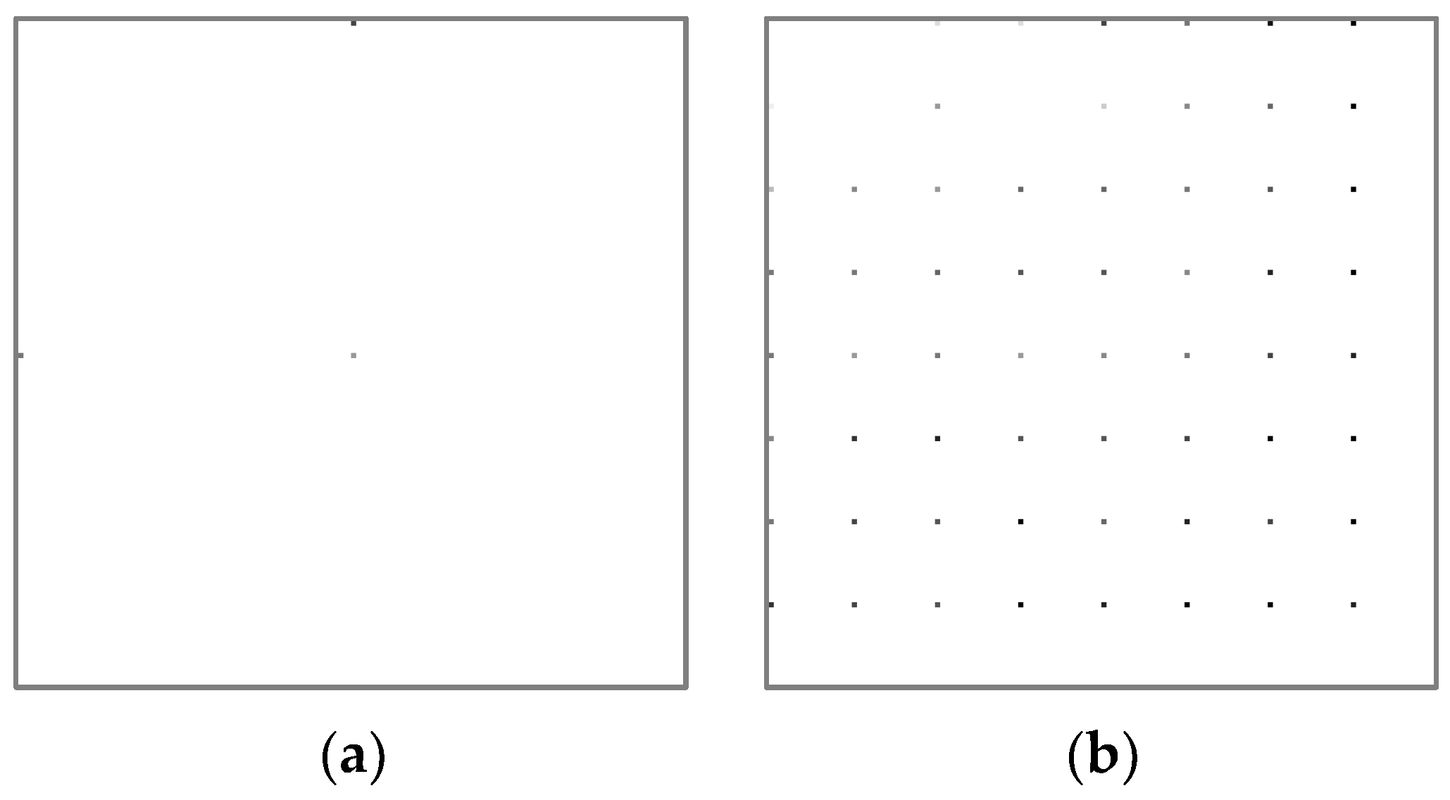
2.3. Measurement of the Box Counting Dimension

2.3.1. Box Counting Analysis of 1-Dimensional Fractals: D_{(Mountain Edge)}

Box counting was performed on the intersection of 1-dimensional fractals with a horizontal line at the trace’s median height. For the 2-dimensional fractal images, a fractal dust set was formed by taking the intersection of the height values of each row of the image with a line intersecting the median height. This dust set was used to compute the box counting dimension through the use of custom Matlab scripts. Briefly, for each box size with side length L, from the length of the fractal to a single pixel in steps of L/2 for a total of n steps, the image is covered with a set of boxes, and the number of boxes that contain any non-zero quantity of points is counted. The box counts of pairs of neighboring grid scales from L/(2³) to L/(2^{n − 3}) were averaged to compute D, while the counts from the grid scales outside this range (the larger and smaller boxes, where n = {0, 1, 2, n − 2, n − 1, and n}), were not used. The embedding dimension of the series of points is 1, but the embedding dimension of the fractal mountain edge is 2, so we averaged these values of D, computed for pairs of grid sizes, and added 1 to report the fractal dimension of the 1-dimensional fractals, D_{(Mountain Edge)}, which span the range 1 < D_{(Mountain Edge)} < 2.

2.3.2. Box Counting Analysis of xy Slices of 2-Dimensional Fractal Coastlines: D_{(Coastal Edge)}

To isolate the coastal edge of a fractal terrain, the median intensity value of the intensity image was selected as the level at which a binary threshold procedure was applied with the Matlab command im2bw. The median, in particular, was selected because it is the level at which all of the resultant binary images have roughly equivalent black and white regions across the range of D. The edge of the binary images was extracted with the Matlab command bwperim. Figure 8 provides examples of the edge extraction process. This particular luminance edge—extracted from the coastal edge images and shown in Figure 8g–i —served as the set on which box counting was performed.

Box counting was performed on the coastal edge images as described in Section 2.3.1, with the exception that the boxes were applied as a grid over the image. Here, the embedding dimension is 2, so for the coastal edge images we report the measured values of D, D_{(Coastal Edge)}, which span the range 1 < D_{(Coastal Edge)} < 2.

2.4. Fourier Decomposition and Measurement of β

2.4.1. Spectral Scaling Analysis of 1-Dimensional Fractals: β_{(Mountain Edge)}

Fractal traces (see examples in Figure 3 and Figure 6e–g) were decomposed with a 1-dimensional Fast Fourier Transform. The square of the real-valued component was retained. Power was plotted against frequency in log–log coordinates, and the slope of a least squares regression line was retained as an empirical measure of the spectral decay rate, β_{(Mountain Edge)}, of the time series.

2.4.2. Spectral Scaling Analysis of 2-Dimensional Fractal Intensity Images: β_(Surface)

Each image was decomposed with a 2-dimensional Fast Fourier Transform. The lowest frequency components were centered, and the square of the real-valued component was retained and transformed into polar coordinates. For each polar angle, power was plotted against frequency in log-log coordinates, and the average was retained as an empirical measure of the spectral decay rate, β_(Surface), of the image (see Figure 9a–c).

3. Results

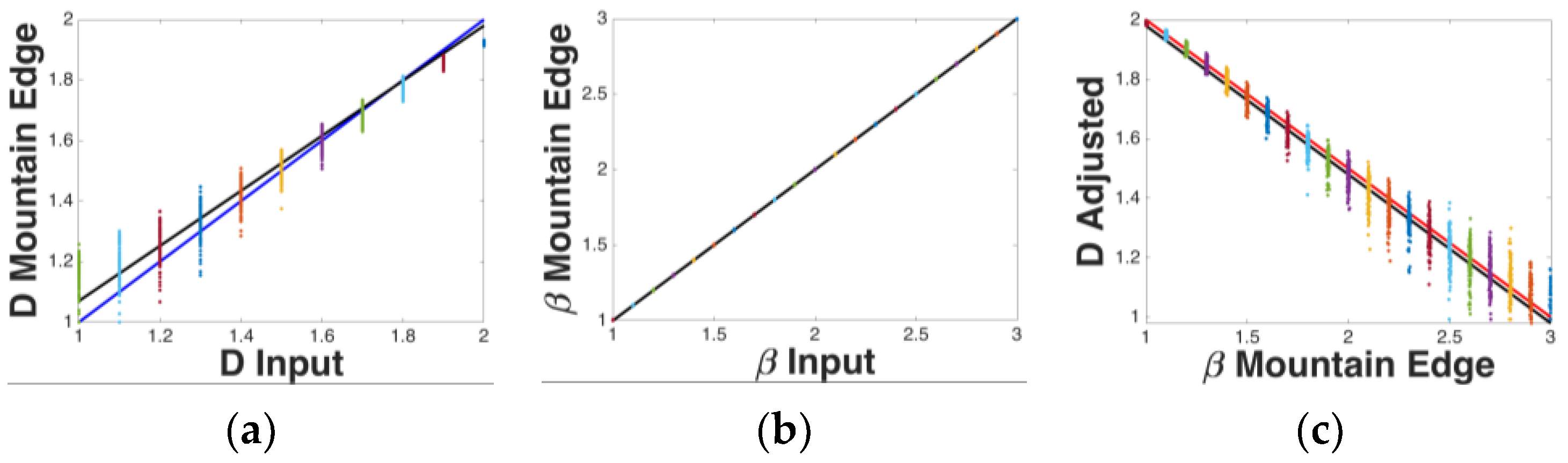
3.1. Relationship between D_{(Mountain Edge)} and β_{(Mountain Edge)} for 1-Dimensional Fractals

We first analyzed 1-dimensional midpoint displacement and Fourier noise fractals to validate our measures and test Voss’s approximation of the relationship between D and β for 1-dimensional fractals. To validate our box counting measure, values of D ranging from 1 to 2 in steps of 0.05 were used to generate 100 sets of midpoint fractals of length 2²⁰. The measurement technique described in Section 2.3.1 over-estimates D by a progressively smaller amount as D approaches 2, as shown in Figure 10a. This is a minor measurement error. Accordingly, the best linear fit, D_(Input) = 0.91 + 0.16 × D_{(Mountain Edge)}, for which R² = 0.97 (Figure 10a, black line), deviates from the unity line (Figure 10a, blue line) by only a small amount.

To validate our spectral scaling rate measure, values of β ranging from 1 to 3 in steps of 0.1 were used to generate 100 sets of fractal Fourier noise of length 2²⁰. The measurement technique described in Section 2.4.1 does well at approximating β (as shown in Figure 10b), with the best linear fit, β_(Input) = 0.0003 + 0.9999 × β_{(Mountain Edge)}, for which R² = 1.00 (Figure 10b, black line), overlapped by the unity line (Figure 10b, blue line).

These measures reliably reflect their input parameters, so we determined the extent to which these empirical measurements are consistent with Voss’s approximation, Equation (5). Because our box counting technique results in a small measurement error across the range of dimension, we adjusted the measured D values of the fractal Fourier noise by substituting D_{(Mountain Edge)} into the experimentally determined regression equation stated above in this section and computing the expected D_(Input), which we call D_(Adjusted) (as shown in Figure 10c). The best linear fit—D_(Adjusted) = 2.48 − 0.50 × β_{(Mountain Edge)}—for which R² = 0.97 (Figure 10c, black line), is close to Voss’s approximation (Equation (5)), given E = 1 (Figure 10c, red line). We conclude that Voss’s approximation for fractals with E < D < E + 1 and 1 < β < 3 is accurate when E = 1. We also note that the difference between Equation (5) and our regression equation is inconsequential, and both overlap our measurements across the range of D and β.

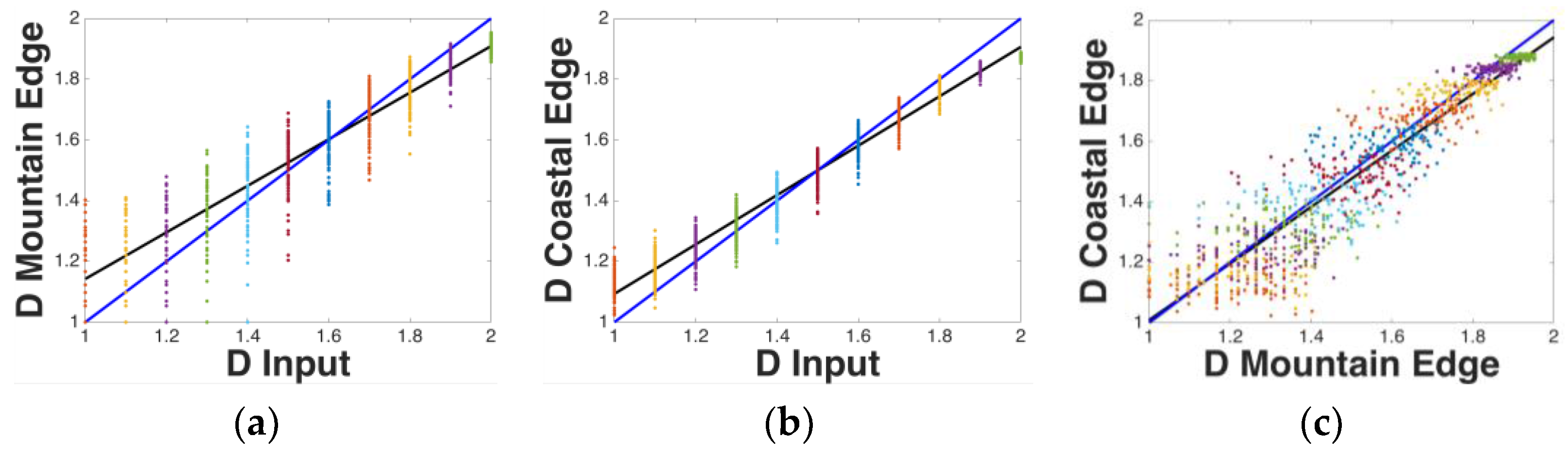
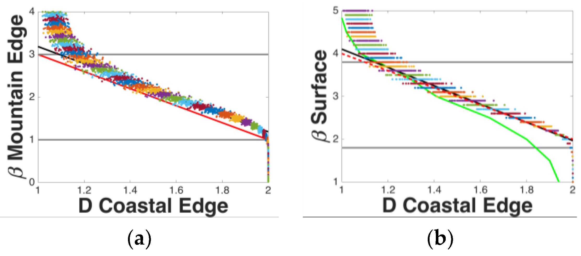
3.2. Relation of D_{(Mountain Edge)} and D_{(Coastal Edge)} for 2-Dimensional Fractals

Voss [5] generalized the relationship between D and β to n-dimensional spaces in Equation (5), so we next consider the case of E = 2, the dimensional space of our visual field. To do so, we first generated 100 sets of midpoint displacement fractals with values of D ranging from 2 to 3 in steps of 0.05 with side length 2¹¹. For each fractal, the dimension of the mountain profile was measured according to the technique described in Section 2.3.1. These measures of D_{(Mountain Edge)} were averaged together for each image. Again, this under- and over-estimates D by a progressively larger amount as D approaches 2 and 1, respectively, as shown in Figure 11a. The best linear fit—D_(Input) = 0.38 + 0.77 × D_{(Mountain Edge)}, for which R² = 0.87 (Figure 11a, black line)—deviates from the unity line (Figure 11a, blue line) in a manner similar to that observed for 1-dimensional fractals. When the coastal edge of the image was measured according to the technique described in Section 2.3.2, we observe a similar trend, with the best linear fit—D_(Input) = 0.28 + 0.81 × D_{(Coastal Edge)}, for which R² = 0.97 (Figure 11b, black line)—deviating from the unity line (Figure 11b, blue line) in a manner similar to that observed for the dust measurement technique. These measures of D, averaged mountain edges and coastal edge values, are reasonable approximations of each other, with the best linear fit D_{(Mountain Edge)} = 0.07 + 0.93 × D_{(Coastal Edge)}, for which R² = 0.86 (Figure 11c). Both of these measures provide an accurate means by which to compute the fractal dimension of an image.

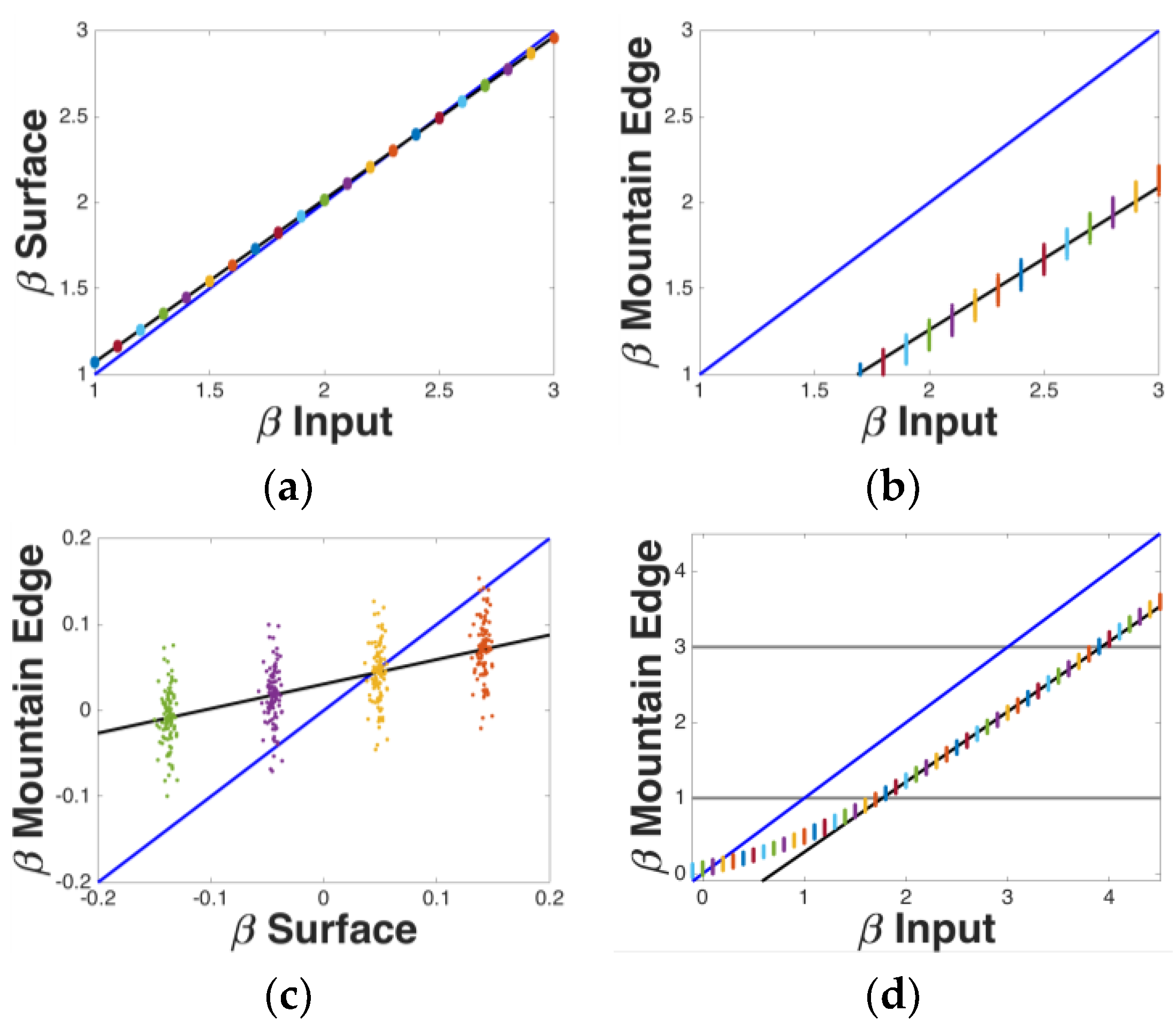
3.3. Relation of β_{(Mountain Edge)} and β_(Surface) for 2-Dimensional Fractals

Having found that our measures of D were consistent with each other, we aimed to test their relation to β. To this end, we generated 100 sets of fractal Fourier noise images with values of β_(Input) ranging from 1 to 3, in steps of 0.1, with side length 2¹¹ pixels. Measuring the spectral decay of a 2-dimensional Fourier analysis as described in Section 2.4.2 provides measured β_(Surface) values that are consistent with the specified input β_(Input) values, with the best linear fit β_(Surface) = 0.12 + 0.95 × β_(Input), for which R² = 0.9999 (see Figure 12a). Having verified the generation process with an analysis in native space, we measured the β of these 2-dimensional fractals along a straight line path, β_{(Mountain Edge)}. We averaged the β_{(Mountain Edge)} measurements for each row of each image, as described in Section 2.4.1, to allow us to follow the definition put forth by Voss [5]. We found that these values of β_{(Mountain Edge)} differ from the specified input β values (see Figure 12b), with an offset as evidenced by the best linear fit β_{(Mountain Edge)} = −0.39 + 0.82 × β_(Input), for which R² = 0.998 (Figure 12b, black line).

We visually inspected the mountain profiles to confirm that their frequency content was indeed different from that implied by β_(Input). We found that the mountain profile from a fractal terrain with an arbitrary value of β_(Surface), β_i, is rougher (i.e., has a larger contribution of fine structure) than a mountain profile from a 1-dimensional fractal with β_{(Mountain Edge)} = β_i (see Figure 13). We then took measurements for an ensemble of 100 random phase maps around β = 0, which show that our measures converge when there is equal power across frequencies (see Figure 12c). An exploratory analysis on a new set of images with 0 ≤ β_(Input) ≤ 4.5 allowed us to empirically determine that fractal Fourier noise terrains with β_(Input) values in the range 1.8 < β_(Input) < 3.8 consistently give β_{(Mountain Edge)} values in the range 1 < β_{(Mountain Edge)} < 3 (see Figure 12d). We found that β_(Input) and β_{(Mountain Edge)} are relatable by the regression equation β_{(Mountain Edge)} = -0.64 + 0.93 × β_(Input), for which R² = 0.997 (Figure 12d, black line), across the range 1 < β_(Mountain) < 3 and 1.8 < β_(Input) < 3.8.

An important validation of our analysis techniques is that β_{(Mountain Edge)} and β_(Surface) approximately converge at β = 0 (as expected), because for white noise, there is equal power across frequencies. This would be trivial if the two measures followed the unity line (Figure 12d, blue line), but certifies that our otherwise non-equivalent measures accurately describe white noise. We note that our β values exhibit slight measurement errors, such that classical Brownian traces (β_{(Mountain Edge)} = 2, β_(Surface) = 3) have empirically determined means of (2.14, 2.95). In the absence of measurement error, the empirically determined range 1.8 < β_(Input) < 3.8 would be 2 < β_(Surface) < 4.

3.4. Relation of β to D for 2-Dimensional Fractals

To relate the two measures of β to D, we generated another 100 sets of fractal Fourier noise with values of β_(Input) ranging from 0 to 5 in steps of 0.1 with side length 2¹¹ pixels.

3.4.1. Relation of β_{(Mountain Edge)} to D_{(Coastal Edge)} of 2-Dimensional Fractals

First, we investigated the extension of Voss’s [5] approximation to E = 2 by determining the relationship between D_{(Coastal Edge)} and β_{(Mountain Edge)}. We performed the Fourier analysis described in Section 2.4.1 on each row of each image, and measured the rows’ fractal dimension with the technique described in Section 2.3.2. The relationship between these measures is described by a best linear fit—β_{(Mountain Edge)} = 5.18 – 2.00 × D_{(Coastal Edge)}, for which R² = 0.99 (Figure 14a, black line)—which approximates Voss’s [5] equation (Figure 14a, red line, which is Equation (5)). This confirms Voss’s [5] assertion that measuring along a straight-line path will provide measures of D and β that are related by Equation (5).

3.4.2. Relation of β_(Surface) to D_{(Coastal Edge)} for 2-Dimensional Fractals

We next measured β using the method described in Section 2.4.2, β_(Surface), which captures the radial scaling properties of the images. When plotted against D_{(Coastal Edge)}, we observe that the relationship between these measures is described by a best linear fit, β_(Surface) = 6.24 − 2.14 × D_{(Coastal Edge)}, for which R² = 0.99 (Figure 14b, black line). The observed relationship agrees with the data from a smaller set of images previously reported by Spehar and Taylor [23] (Figure 14b, green line). Significantly, this observed relationship between β_(Surface) and D_{(Coastal Edge)} agrees with Equation (11) which we present below, and will allow conversion across measures of D and β in multidimensional spaces.

4. Discussion

4.1. Mathematical Relationships between Ds and βs

Our results show that Voss [5] was correct regarding Equation (5)’s extension into n-dimensional measures of D with the limitations described therein. However, the way that β is commonly measured in images, β_(Surface), is not that which Voss [5] described. Voss’s [5] equation (Equation (5)) applies for the measure we call β_{(Mountain Edge)}. However, vision researchers typically use β_(Surface). Whereas the difference between these two spectral decay rates is nonexistent for white noise, where β = 0, these measures are substantially different in the range over which these noises are fractal. Before commenting further on the different measures of β, we will first summarize the relationships for the fractal images discussed in this paper.

For the mountain profile fractal (E = 1), the Voss relationship of Equation (5) becomes:

D_{(Mountain Edge)} = 1 + (3 − β_{(Mountain Edge)})/2

(6)

We have also shown in Section 3.3 that the Fourier spectral decay rates measured in 1- and 2-dimensional space are approximately related by:

β_{(Mountain Edge)} = β_(Surface) − 1

(7)

over the range 1 < β_{(Mountain Edge)} < 3 and 2 < β_(Surface) < 4. Combining Equations (6) and (7) gives:

D_{(Mountain Edge)} = 1 + (4 − β_(Surface))/2

(8)

The relationship between β and D_(Surface) can then be obtained using:

D_(Surface) = D_{(Mountain Edge)} + 1 = D_{(Coastal Edge)} + 1

(9)

We have not measured β_{(Coastal Edge)} in our investigations. However, we expect that, if a coastal edge was unraveled by the process described by Zahn & Roskies [48], its β value will equal β_{(Mountain Edge)} because D_{(Coastal Edge)} is equivalent to D_{(Mountain Edge)} and E = 1 applies to both the mountain and coastal edges.

4.2. Distinguishing βs

Our results provide the ranges of β over which the images are fractal. As Voss [5] noted, for D mountain (1 < D_{(Mountain Edge)} < 2), we have 1 < β_{(Mountain Edge)} < 3. However, we have shown that β measured in a single variable-space (i.e., along a straight line path as β_{(Mountain Edge)}) diverges from β measured in a two-variable space (i.e., across a plane as β_(Surface)) to an extent that is characterized by Equation (7) for the range over which 2-dimensional noise is fractal. For D surface (2 < D_(Surface) < 3), we have 2 < β_(Surface) < 4 and 1 < β_{(Mountain Edge)} < 3. The fact that the β values measured by 1- and 2-dimensional Fourier transforms differ for fractal noises holds crucial consequences. The fractal structure of a terrain is quantified by β_{(Mountain Edge)}. Visual inspection of Figure 13 makes it immediately apparent that its value is significantly smaller than β_(Surface) for fractals of topological dimension E = 2. Given that β_(Input) matches β_(Surface) rather than β_{(Mountain Edge)}, it is likely that many vision researchers have been misjudging the fractal content of their fractal terrains, or adapting them by an intuitive sense of the image’s roughness. Equation (7) provides a formal justification for adjusting the β of 2-dimensional fractals.

The basis for this conversion lies in the difference in generating 1- vs. 2-dimensional noise. A pair of vectors can specify the phases and amplitudes of a 1-dimensional fractal noise pattern because they have only one phase at each frequency (for illustration, see the visualization of the amplitude vectors corresponding to three different input Betas (β_is) shown in Figure 6a–c and phase matrix shown in Figure 6d). In contrast, a 2-dimensional fractal pattern is generated from a matrix of amplitudes and a matrix of phases (for illustration, see the visualization of the amplitude matrices corresponding to three different input Betas (β_is) shown in Figure 7a–c and phase matrix shown in Figure 7d).

For 2- and higher-dimensional fractal noises, there are an increasingly greater number of inputs at increasingly high spatial frequencies (for illustration, see Figure 15, where the lowest frequency components have been centered). The number of inputs increases at a rate that is related to the distance from the lowest frequency (i.e., the radial distance in a low-spatial frequency-centered representation of Fourier space). Changing from a 1- to 2-variable space, weighting the input function S_V(f) by f to increase the embedding dimension by 1 (from 1 to 2) requires a subtraction of 1 from β, as denoted by the following equation:

S_V(f) × f = (f^−β_i) × f = 1/f^(β_i ^{− 1)}

(10)

4.3. A Generalized Equation to Relate Ds and βs

We postulate that the relationship between D and β continues to change with higher dimensional Fourier decomposition (for 3- and higher dimensional Fourier decomposition), such that the relationship between D and β can be described by the equation,

D = E + (F + 2 − β)/2

(11)

where F is the dimensional space of the Fourier transform (the number of variables with which the Fourier transform is performed), where F ≥ 1, and F < β < F + 2 (as examples, F = 1 for β_{(Mountain Edge)} and F = 2 for β_(Surface)). This new equation (Equation (11)) allows for conversion from D to both of the Fourier measurement techniques that can describe static images, and provides an extension of Mandelbrot’s [1,4], Voss’s [5], and Knill et al.’s [14] relationships that can describe spectral decay in dynamic fractal Brownian stimuli generated with Fourier, midpoint displacement, and other equivalent methods. Equation (11) extends Voss’s [5] equation (Equation (5)) by generalizing the term for β from β_{(Mountain Edge)}.

4.4. Importance of the Relationship between D and β for Current and Future Research

In addition to allowing for easy translation across the parameters D and β in aesthetics research, Equation (11) provides scaffolding for extension of basic vision research into questions related to visual sensitivity and the perception of fractal motion, and has far-reaching applicability to applied topics, including stress reduction and navigation.

To clarify the need for this new equation to allow for such forward progress, consider a hypothetical case of therapeutic intervention using fractal movies. From Equation (5) and previous research that suggests that low-to-moderate fractional dimensions (1.3 ≤ D ≤ 1.5) are optimal for stress reduction [49], a therapist might generate what are intended to be soothing movies of fractal noise with β = 2.2, thinking that β does not differ according to the number of variables with which the Fourier transform is performed. Meanwhile, the results of our analyses imply that such a series would be effectively space filling if β_(Volume) = 2.2. This is because Equation (11) implies the optimal range of values of β_(Volume) for such an application would be 4 < β_(Volume) < 4.4, because E = 3 and F = 3, where fractal noises are in the range 3 < β_(Volume) < 5.

More generally, time represents a third dimension—yet to be explored—in the perception of fractal processes. An example would be a fractal pattern that undergoes fractal change over time. Responses to dynamic stimuli have a long history of consideration in vision research that continues today [50,51], though few have focused on perception of fractal motion [52,53]. Equation (11) provides the scaffolding to extend perceptual research into the study of dynamic fractals.

While Equation (11) supports the development of new lines of work into dynamic fractals, it also holds value in drawing conclusions across recent research using 2-dimensional fractal patterns in studies that have implications for aesthetics. Whereas Rainville and Kingdom [54] provide βs that are apparently in terms of β_{(Mountain Edge)}, they cite Knill et al. [14], who provided the relationship between D and β for surfaces. This highlights the difficulty associated with discerning the optimal range of β in aesthetics and vision research. More problematic is that because of the relative convenience of the respective algorithms’ implementation, others report a combination of D_{(Mountain Edge)} and β_(Surface) values [23], for which there is no clear conversion provided in the published literature.

Finally, Equation (11) serves as a useful tool for converting between 2- and 3-dimensional representations of space, the problem we solve whenever we use a map to navigate. The recent work of Juliani et al. [28] asks individuals to navigate fractal environments. Under conditions such as these, the map typically has complexity in the range 1 < D_{(Coastal Edge)} < 2, whereas the navigated environment has complexity in the range 2 < D_(Surface) < 3, and the visually perceived scene has a spectral decay that likely falls off at a rate in the range 2 < β_(Surface) < 4. While it is mathematically no less appropriate to describe all of these in terms of β_{(Mountain Edge)}, it is easier to interpret results described in units that reflect the experienced dimensional space precisely and explicitly. There is convenience to be gained by using this more general equation (Equation (11)) and its variables’ boundary conditions rather than more specialized equations, such as those which have been put forth previously [5,14,21]. Equation (11) stems from a recognition that β varies with the number of variables with which the Fourier transform is applied. As such, it is important that we define which β is being used (β_(Line), β_(Surface), β_(Volume), etc.) for easier interpretation of results and to facilitate the communication of future endeavors in interdisciplinary fractals research.

References

1. Mandelbrot, B.B. Fractals: Form, Chance, and Dimension; Freeman: San Francisco, CA, USA, 1977. [Google Scholar]
2. Fournier, A.; Fussel, D.; Carpenter, L. Computer rendering of stochastic models. Commun. ACM 1982, 25, 371–384. [Google Scholar] [CrossRef]
3. Saupe, D. Algorithms for random fractals. In The Science of Fractal Images; Peitgen, H., Saupe, D., Eds.; Springer-Verlag: New York, NY, USA, 1982; pp. 71–136. [Google Scholar]
4. Mandelbrot, B.B. The Fractal Geometry of Nature; Freeman: San Francisco, CA, USA, 1983. [Google Scholar]
5. Voss, R.F. Characterization and measurement of random fractals. Phys. Scripta 1986, 13, 27–32. [Google Scholar] [CrossRef]
6. Fairbanks, M.S.; Taylor, R.P. Scaling analysis of spatial and temporal patterns: From the human eye to the foraging albatross. In Non-Linear Dynamical Analysis for the Behavioral Sciences Using Real Data; Taylor & Francis Group: Boca Raton, FL, USA, 2011. [Google Scholar]
7. Avnir, D.; Biham, O.; Lidar, D.; Malci, O. Is the geometry of nature fractal? Science 1998, 279, 39–40. [Google Scholar] [CrossRef]
8. Mandelbrot, B.B. Is nature fractal? Science 1998, 279, 738. [Google Scholar] [CrossRef]
9. Jones-Smith, K.; Mathur, H. Fractal analysis: Revisiting Pollock’s drip paintings. Nature 2006, 444, E9–E10. [Google Scholar] [CrossRef] [PubMed]
10. Taylor, R.P.; Micolich, A.P.; Jonas, D. Fractal analysis: Revisiting Pollock’s drip paintings (Reply). Nature 2006, 444, E10–E11. [Google Scholar] [CrossRef]
11. Markovic, D.; Gros, C. Power laws and self-organized criticality in theory and nature. Phys. Rep. 2014, 536, 41–74. [Google Scholar] [CrossRef]
12. Burton, G.J.; Moorehead, I.R. Color and spatial structure in natural scenes. Appl. Opt. 1987, 26, 157–170. [Google Scholar] [CrossRef] [PubMed]
13. Field, D.J. Relations between the statistics of natural images and the response properties of cortical cells. J. Opt. Soc. Am. A 1987, 4, 2379. [Google Scholar] [CrossRef] [PubMed]
14. Knill, D.C.; Field, D.; Kersten, D. Human discrimination of fractal images. J. Opt. Soc. Am. A 1990, 7, 1113–1123. [Google Scholar] [CrossRef] [PubMed]
15. van Hateren, J.H. Theoretical predictions of spatiotemporal receptive fields of fly LMCs, and experimental validation. J. Comp. Physiol. A 1992, 171, 157–170. [Google Scholar] [CrossRef]
16. Tolhurst, D.J.; Tadmor, Y.; Chao, T. Amplitude spectra of natural images. Ophthalmic Physiol. Opt. 1992, 12, 229–232. [Google Scholar] [CrossRef] [PubMed]
17. Field, D.J. Scale-invariance and self-similar wavelet transforms: An analysis of natural scenes and mammalian visual systems. In Wavelets, Fractals, and Fourier Transforms; Farge, M., Hunt, J.C.R., Vassilicos, J.C., Eds.; Clarendon Press: Oxford, UK, 1993; pp. 151–193. [Google Scholar]
18. Ruderman, D.L.; Bialek, W. Statistics of natural images: Scaling in the woods. Phys. Rev. Lett. 1994, 73, 814–817. [Google Scholar] [CrossRef] [PubMed]
19. Ruderman, D.L. Origins of scaling in natural images. Vis. Res. 1996, 37, 3385–3398. [Google Scholar] [CrossRef]
20. van der Schaaf, A.; van Haternen, J.H. Modeling the power spectra of natural images: Statistics and information. Vis. Res. 1996, 36, 2759–2770. [Google Scholar] [CrossRef]
21. Graham, D.J.; Field, D.J. Statistical regularities of art images and natural scenes: Spectra, sparseness, and nonlinearities. Spat. Vis. 2007, 21, 149–164. [Google Scholar] [CrossRef] [PubMed]
22. Hagerhall, C.M.; Purcell, T.; Taylor, R. Fractal dimension of landscape silhouette outlines as a predictor of landscape preference. J. Environ. Psychol. 2004, 24, 247–255. [Google Scholar] [CrossRef]
23. Spehar, B.; Taylor, R.P. Fractals in art and nature: Why do we like them? In Proceedings of the SPIE 8651, Human Vision and Electronic Imaging XVIII, 865118, Burlingame, CA, USA, 3 February 2013.
24. Spehar, B.; Wong, S.; van de Klundert, S.; Lui, J.; Clifford, C.W.G.; Taylor, R.P. Beauty and the beholder: The role of visual sensitivity in visual preference. Front. Hum. Neurosci. 2015, 9, 514. [Google Scholar] [CrossRef] [PubMed]
25. Bies, A.J.; Blanc-Goldhammer, D.R.; Boydston, C.R.; Taylor, R.P.; Sereno, M.E. Aesthetic responses to exact fractals driven by physical complexity. Front. Hum. Neurosci. 2016, 10, 210. [Google Scholar] [CrossRef] [PubMed]
26. Street, N.; Forsythe, A.M.; Reilly, R.; Taylor, R.; Helmy, M.S. A complex story: Universal preference vs. individual differences shaping aesthetic response to fractals patterns. Front. Hum. Neurosci. 2016, 10, 213. [Google Scholar] [CrossRef] [PubMed]
27. Spehar, B.; Walker, N.; Taylor, R.P. Taxonomy of individual variations in aesthetic responses to fractal patterns. Front. Hum. Neurosci. 2016, 10, 350. [Google Scholar] [CrossRef]
28. Juliani, A.W.; Bies, A.J.; Boydston, C.R.; Taylor, R.P.; Sereno, M.E. Navigation performace in virtual environments varies with the fractal dimension of the landscape. J. Environ. Psychol. 2016, 47, 155–165. [Google Scholar] [CrossRef] [PubMed]
29. Bies, A.J.; Kikumoto, A.; Boydston, C.R.; Greenfield, A.; Chauvin, K.A.; Taylor, R.P.; Sereno, M.E. Percepts from noise patterns: The role of fractal dimension in object pareidolia. In Vision Sciences Society Meeting Planner; Vision Sciences Society: St. Pete Beach, FL, USA, 2016. [Google Scholar]
30. Field, D.; Vilankar, K. Finding a face on Mars: A study on the priors for illusory objects. In Vision Sciences Society Meeting Planner; Vision Sciences Society: St. Pete Beach, FL, USA, 2016. [Google Scholar]
31. Hagerhall, C.M.; Laike, T.; Kuller, M.; Marcheschi, E.; Boydston, C.; Taylor, R.P. Human physiological benefits of viewing nature: EEG responses to exact and statistical fractal patterns. Nonlinear Dyn. Psychol. Life Sci. 2015, 19, 1–12. [Google Scholar]
32. Isherwood, Z.J.; Schira, M.M.; Spehar, B. The BOLD and the Beautiful: Neural responses to natural scene statistics in early visual cortex. i-Perception 2014, 5, 345. [Google Scholar]
33. Bies, A.J.; Wekselblatt, J.; Boydston, C.R.; Taylor, R.P.; Sereno, M.E. The effects of visual scene complexity on human visual cortex. In Society for Neuroscience, Proceedings of the 2015 Neuroscience Meeting Planner, Chicago, IL, USA, 21 October 2015.
34. Sprott, J.C. Automatic generation of strange attractors. Comput. Graph. 1993, 17, 325–332. [Google Scholar] [CrossRef]
35. Aks, D.J.; Sprott, J.C. Quantifying aesthetic preference for chaotic patterns. Empir. Stud. Arts 1996, 14, 1–16. [Google Scholar] [CrossRef]
36. Spehar, B.; Clifford, C.W.; Newell, B.R.; Taylor, R.P. Universal aesthetic of fractals. Comput. Graph. 2003, 27, 813–820. [Google Scholar] [CrossRef]
37. Taylor, R.P.; Spehar, B.; Van Donkelaar, P.; Hagerhall, C. Perceptual and physiological responses to Jackson Pollock’s fractals. Front. Hum. Neurosci. 2011, 5, 60. [Google Scholar] [CrossRef] [PubMed]
38. Mureika, J.R.; Dyer, C.C.; Cupchik, G.C. Multifractal structure in nonrepresentational art. Phys. Rev. E 2005, 72, 046101. [Google Scholar] [CrossRef] [PubMed]
39. Forsythe, A.; Nadal, M.; Sheehy, N.; Cela-Conde, C.J.; Sawey, M. Predicting beauty: Fractal dimension and visual complexity in art. Br. J. Psychol. 2011, 102, 49–70. [Google Scholar] [CrossRef] [PubMed] [Green Version]
40. Hagerhall, C.M.; Laike, T.; Taylor, R.P.; Kuller, M.; Kuller, R.; Martin, T.P. Investigations of human EEG response to viewing fractal patterns. Perception 2008, 37, 1488–1494. [Google Scholar] [CrossRef] [PubMed]
41. Graham, D.J.; Redies, C. Statistical regularities in art: Relations with visual coding and perception. Vis. Res. 2010, 50, 1503–1509. [Google Scholar] [CrossRef] [PubMed]
42. Koch, M.; Denzler, J.; Redies, C. 1/f 2 characteristics and isotropy in the fourier power spectra of visual art, cartoons, comics, mangas, and different categories of photographs. PLoS ONE 2010, 5, e12268. [Google Scholar] [CrossRef] [PubMed]
43. Melmer, T.; Amirshahi, S.A.; Koch, M.; Denzler, J.; Redies, C. From regular text to artistic writing and artworks: Fourier statistics of images with low and high aesthetic appeal. Front. Hum. Neurosci. 2013, 7, 106. [Google Scholar] [CrossRef] [PubMed]
44. Dyakova, O.; Lee, Y.; Longden, K.D.; Kiselev, V.G.; Nordstrom, K. A higher order visual neuron tuned to the spatial amplitude spectra of natural scenes. Nat. Commun. 2015, 6, 8522. [Google Scholar] [CrossRef] [PubMed]
45. Menzel, C.; Hayn-Leichsenring, G.U.; Langner, O.; Wiese, H.; Redies, C. Fourier power spectrum characteristics of face photographs: Attractiveness perception depends on low-level image properties. PLoS ONE 2015, 10, e0122801. [Google Scholar]
46. Braun, J.; Amirshahi, S.A.; Denzler, J.; Redies, C. Statistical image properties of print advertisements, visual artworks, and images of architecture. Front. Psychol. 2013, 4, 808. [Google Scholar] [CrossRef] [PubMed]
47. Cutting, J.E.; Garvin, J.J. Fractal curves and complexity. Percept. Psychophys. 1987, 42, 365–370. [Google Scholar] [CrossRef] [PubMed]
48. Zahn, C.T.; Roskies, R.Z. Fourier descriptors for plane closed curves. IEEE Trans. Comput. 1972, 3, 269–281. [Google Scholar] [CrossRef]
49. Taylor, R.P. Reduction of physiological stress using fractal art and architecture. Leonardo 2006, 39, 245–251. [Google Scholar] [CrossRef]
50. Derrington, A.M.; Allen, H.A.; Delicato, L.S. Visual mechanisms of motion analysis and motion perception. Ann. Rev. Psychol. 2004, 55, 181–205. [Google Scholar] [CrossRef] [PubMed]
51. Silies, M.; Gohl, D.M.; Clandinin, T.R. Motion-detecting circuits in flies: Coming into view. Ann. Rev. Neurosci. 2014, 37, 307–327. [Google Scholar] [CrossRef] [PubMed]
52. Benton, C.P.; O’Brien, J.M.; Curran, W. Fractal rotation isolates mechanisms for form-dependent motion in human vision. Biol. Lett. 2007, 3, 306–308. [Google Scholar] [CrossRef] [PubMed]
53. Lagacé-Nadon, S.; Allard, R.; Faubert, J. Exploring the spatiotemporal properties of fractal rotation perception. J. Vis. 2009, 9. [Google Scholar] [CrossRef] [PubMed]
54. Rainville, S.J.; Kingdom, F.A.A. Spatial scale contribution to the detection of symmetry in fractal noise. JOSA A 1999, 16, 2112–2123. [Google Scholar] [CrossRef] [PubMed]
Figure 1. Plots of a fractal terrain with D = 2.5 and its intersection with axial planes; (a) “Surface” plot of a fractal terrain; (b) intensity “image” of the terrain; (c) “mountain edge” profile of an “xz-slice” or “yz-slice” of the terrain; (d) “coastal edge” of an “xy-slice” of the terrain.
Symmetry 08 00066 g001
Figure 2. Illustration of the generation of 1-dimensional midpoint displacement fractals. (a) Cartoon graph of a scaling plot in log–log coordinates that determines the rate of scaling of midpoint displacements across recursions for high (solid line) and low (dashed line) D fractals; (b) Schematics of recursions 0–2 are shown for low (dashed line) and high (solid line) D exact midpoint displacement fractals. Gray arrows indicate displacements that occur with each recursion in (b).
Symmetry 08 00066 g002
Figure 3. Plots of 1-dimensional statistical midpoint displacement fractals. (ac) Fractal traces that vary in D, such that D = 1.2, 1.5, and 1.8, are generated from a single set of random numbers that contribute to the variable length and direction of displacement of the midpoints at each recursion.
Symmetry 08 00066 g003
Figure 4. Illustration of the generation of a 2-dimensional midpoint displacement fractal as the heights (indicated by grayscale intensity) of particular points are specified over eight recursions. (ad) The second, fourth, sixth, and final recursions are shown. In (ac), white space indicates points for which height has not yet been specified.
Symmetry 08 00066 g004aSymmetry 08 00066 g004b
Figure 5. Plots of 2-dimensional midpoint displacement fractals. (ac) Surface plots of fractals generated from a single set of random numbers that vary in D, such that D = 1.2, 1.5, and 1.8; (df) Grayscale intensity map images of the surface plots in (ac).
Symmetry 08 00066 g005
Figure 6. Generation of 1-dimensional Fourier noise fractals. (ac) Power (y-axis) as a function of frequency (x-axis) for β(Input) = 2.6, 2, and 1.4; (d) Set of random phases (y-axis) as a function of frequency (x-axis); (eg) fractal traces resulting from the pairing of the phases in panel (d) with power spectra from (a–c) respectively.
Symmetry 08 00066 g006
Figure 7. Generation of 2-dimensional Fourier noise fractals. (ac) Power (z-axis) as a function of frequency in xy coordinates for β(Input) = 2.6, 2, and 1.4; (d) Set of random phases (z-axis) as a function of frequency in xy coordinates; (eg) fractal terrains resulting from the pairing of the phases in panel (d) with power spectra from (a–c) respectively.
Symmetry 08 00066 g007
Figure 8. Edge extraction procedure for 2-dimensional midpoint displacement fractals. (ac) Grayscale intensity map images of fractals generated from a single set of random numbers that vary in D, such that D = 1.2, 1.5, and 1.8; (df) Binary images resulting from the threshold procedure applied to the terrains shown in (ac); (gi) Coastal edges extracted from the binary images shown in (df).
Symmetry 08 00066 g008
Figure 9. Fourier decomposition of 2-dimensional fractals. (a) Fractal surface generated with the inverse Fourier method; (b) Power spectrum of the Fourier decomposition of the terrain shown in (a); (c) Power spectrum shown in (b) with low spatial frequencies centered.
Symmetry 08 00066 g009
Figure 10. 1-dimensional fractal measurements. (a) Midpoint displacement fractals’ D(Mountain Edge) measurements plotted against their D(Input) values; (b) Fourier noise fractals’ β(Mountain Edge) measurements plotted against their β(Input) values; (c) Fourier noise fractals’ D(Mountain Edge) measurements, adjusted by the linear fit from panel (a), plotted against their β(Mountain Edge) measurements. In each panel, the best linear fit for the data is shown with a black line. In panels (a,b), unity is represented by the blue line. In panel (c), Voss’s approximation (Equation (5)) is represented by the red line. Data are colored to distinguish adjacent input values such that each datum's color is determined by D(Input) in panel (a) and β(Input) in panels (b,c).
Symmetry 08 00066 g010
Figure 11. 2-dimensional fractal D measurements. (a) Midpoint displacement fractals’ D(Mountain Edge) measurements plotted against their D(Input) values; (b) Midpoint displacement fractals’ D(Coastal Edge) measurements plotted against their D(Input) values; (c) Midpoint displacement fractals’ D(Coastal Edge) measurements plotted against their D(Mountain Edge) measurements. In each panel, unity is represented by the blue line, while the best linear fit for the data is represented by the black line. Data are colored to distinguish adjacent input values such that each datum's color is determined by D(Input) in panels (a–c).
Symmetry 08 00066 g011
Figure 12. 2-dimensional fractal β measurements. (a) Fourier noise fractals’ β(Surface) measurements plotted against their β input values; (b) Fourier noise fractals’ β(Mountain Edge) measurements plotted against their β(Input) values; (c) Fourier noise fractals’ β(Mountain Edge) measurements plotted against their β(Surface) measurements, showing that the measures converge at β = 0; (d) Fourier noise fractals’ β(Mountain Edge) measurements plotted against their β(Input) values. In each panel, unity is represented by the blue line, while the best linear fit for the data is represented by the black line. Data are colored to distinguish adjacent input values such that each datum's color is determined by β(Input) in panels (a–d).
Symmetry 08 00066 g012
Figure 13. Mountain profiles from 1 and 2-dimensional fractal Fourier noise. (a) 1-dimensional fractal with β(Input) = 1.5; (b) 1-dimensional fractal with βInput = 2.5; (c) 2-dimensional fractal with β(Input) = 2.5; (d) 1-dimensional fractal mountain edges from the terrain in (c).
Symmetry 08 00066 g013
Figure 14. 2-dimensional fractal measurements of Fourier noise (a,b). (a) Fourier noise fractals’ β(Mountain Edge) measurements plotted against their D(Coastal Edge) measurements; (b) Fourier noise fractals’ β(Surface) measurements plotted against their D(Coastal Edge) measurements. In each panel, the best linear fit for the data within the region that was shown to exhibit fractal scaling (identified with gray lines) is shown with a black line. In panel (a), Voss’s [5] equation (Equation (5)) is shown with a red line. In panel (b), Spehar & Taylor’s [23] data is shown with a green line and our extension of Voss’s [5] equation (Equation (11)) is shown with a red dashed line. Data are colored to distinguish adjacent input values such that each datum's color is determined by β(Input) in panels (a,b).
Symmetry 08 00066 g014
Figure 15. Real and imaginary frequency components of 1- and 2-dimensional fractal Fourier noise plotted in 2- and 3-dimensional spaces with color changing with frequency, such that higher frequency components are shown in cooler colors. (a,b) Amplitude-frequency plots of a 1-dimensional noise with low frequency components centered such that the amplitude of the higher frequency components fall at the edges of the plot; (c,d) Amplitude-frequency plots of 2-dimensional noise with low frequency components centered such that larger concentric circles indicate higher frequency components.
Symmetry 08 00066 g015