Broken versus Non-Broken Time Reversal Symmetry: Irreversibility and Response

Abstract

We review some approaches to macroscopic irreversibility from reversible microscopic dynamics, introducing the contribution of time dependent perturbations within the framework of recent developments in non-equilibrium statistical physics. We show that situations commonly assumed to violate the time reversal symmetry (presence of magnetic fields, rotating reference frames, and some time dependent perturbations) in reality do not violate this symmetry, and can be treated with standard theories and within standard experimental protocols.

1. Introduction

Temporal irreversibility is one of the classic questions of physics, particularly because it deals with the most common experience of our daily life, but it looks at odds with our understanding of the properties of the microscopic constituents of matter. Since men first observed movement and mutation in nature, they learned that things generally happen in a preferential direction, like they are carried on by some active principles that follow a rigorous arrow of time. A stone rolling down the hill would never be seen at the top again (unless an external agent takes it back), just like a hot body in contact with a colder one will cool down by transferring heat to the other and not vice versa. Possibly more evident is the psychological arrow of time: we can remember the past but not the future, and physicists of course make no exception to that. Nevertheless, the standard picture of the microscopic dynamics, concerning atoms and molecules of which matter is made, is time reversal invariant. Given a container filled up with a gas of N interacting molecules, each characterized by position q and momentum p, this picture assumes that one can invert (at least in principle) all the momenta of these particles keeping their absolute values fixed. The ensuing evolution would then trace back the forward trajectory with reversed momenta. This means that we can consider as equally possible two opposite evolutions, merely resulting from different initial conditions. Therefore, there seems to be no hint of irreversibility at this level of description of the physical world.

Around 1865, Clausius arguably made the first attempt to characterize irreversibility as a physical phenomenon, introducing the concept of entropy [1], a totally new thermodynamic variable providing a constraint for spontaneous macroscopic processes. Entropy never decreases in an isolated system—it either increases or remains the same—and its growth then constitutes a measure of irreversibility at the macroscopic level. This idea proved to be physically extremely accurate and practically very useful, hence Boltzmann tried to frame it within the atomistic description of matter, which he strongly supported. His famous H-theorem was meant to prove that the second law of thermodynamics is consistent and can actually be derived from the microscopic point of view.

In our discussion of time irreversibility, two things seem particularly important in Boltzmann’s argument: first of all, the totally new statistical flavour of the molecular chaos hypothesis used by Boltzmann in deriving his renowned kinetic equation. Boltzmann argued that, for a rarefied gas of particles, the joint probability distribution of positions and momenta can be factorized in the product of single-particle distributions, which means that correlations between interacting particles must decay after some short time due to collisions. This merely statistical idea of loss of memory, being alien to classical mechanics, was hardly acceptable for most of the scientists of that period. Indeed, Boltzmann’s probabilistic approach apparently abandoned the rigorous laws of mechanics, believed to explain all natural phenomena, in order to accept the apparently more vague laws of probability, to account for the fact that we are just limited observers in the world. In addition, the existence of different scales of observation implied by this approach could have (erroneuosly) raised the doubt that a degree of subjectivity was introduced in physics. This was particularly hard to accept at a time in which the very existence of atoms was still debated.

The second important aspect of Boltzmann’s reasoning is outlined by Carlo Cercignani [2]: the validity of the kinetic equation is based on the requirement of smoothness of the distribution function at the initial time, and on the assumption that this smoothness persists in time. This argument has the deep significance that the kinetic equation describes a system evolving towards more and more homogeneous distributions (states of disorder), rather than toward more inhomogeneous ones. This statement reflects the molecular chaos hypothesis: if the evolution, in fact, went from a disordered state to an ordered one, this would imply a strong correlation between particles entering a collision.

So why does the kinetic equation remain one of the most fundamental and succesful equations of physics, despite its apparently rather limited domain of applicability? This question leads to the very core of the dissertation: for a macroscopic system close to equilibrium, the dynamics captured by the Boltzmann equation, which is relaxation towards states of higher and higher disorder, are the only physically significant ones.

This irreversible trend toward homogeneity does not derive directly from classical mechanics laws, since they are perfectly reversible. It is the consequence of: (1) the fact that, at the macroscpic level, we do not distinguish different microscopic disordered configurations; and (2) the quality of initial states.

This paper is organized as follows. In Section 2, we discuss the standard approach to irreversibility for a single macroscopic system whose microscopic dynamics is time reversal invariant (TRI), pointing out some of its limitations. In Section 3, we introduce the theory of non-equilibrium dissipative systems, emphasizing the role of the Dissipation Function, among other recent results. In Section 4, we illustrate the use of the dissipation function in the context of a general theory of dynamical systems, and we develop the theory required to treat time dependent perturbations and to their connections with the steady-state Fluctuation Relations. In Section 4.3, we derive the t-mixing condition for non-equilibrium systems relaxing to steady states, and we point out its implications for the problem of the irreversibility of TRI microscopic dynamics. Section 5 contains our concluding remarks. We also include an appendix with some mathematical details on the derivation of results that appear in Section 4.

2. Standard Picture for Irreversible Relaxation to Equilibrium

We begin illustrating Boltzmann’s approach to irreversible relaxation to equilibrium that has been considered for a gas that expands from an initially compressed state until it fills its container. The main physical ingredients of this approach are: (a) the enormous number of particles that constitute the gas; (b) the fact that these particles interact, so that their velocities are randomized; and (c) the interaction energy is negligible compared to the kinetic energy of the system.

The mathematical theory assumes, cf. Reference [3,4], that the microscopic constituents of the gas are described by Hamiltonian dynamics in a phase space $\mathcal{M}$ and that the measurement of an observable O selects a certain subvolume of $\mathcal{M}$, namely the set of phases that are compatible with the experimentally obtained numerical values. It turns out that volumes corresponding to the equilibrium values of the observables of interest are overwhelmingly larger than volumes corresponding to non-equilibrium values. Therefore, a system evolving spontaneously and without constraints in $\mathcal{M}$ finds it practically impossible to avoid the equilibrium region or to exit from it. Because the dynamics continue forever, the phase space trajectory may fluctuate outside the equilibrium region, but these are going to be exceedingly rare and quickly vanishing events.

Equilibrium microstates are thus called typical, in the sense that they constitute almost entirely the phase space, i.e., with the exception of phases of vanishing volume. Because the Liouville measure on $\mathcal{M}$, μ say, is preserved by these conservative dynamics, typicality also means that the exceptions to the most common behaviour constitute a set of zero μ-measure [The roles of phase space volumes and of the Liouville measure, however, ought not to be confused [5]. In addition, observe that this notion of typicality is mathematically convenient, but it does not need to be exactly verified by systems of physical interest; in particular, Khinchin’s ergodic theory implies that a proper description of a macroscopic object may include a small but positive volume of trajectories with different behaviours [6]].

To explain how this can be the case, combinatorial calculus over finite state spaces is often invoked. For instance, consider a system whose states are represented by strings of N symbols, $X^{\left(N\right)}=(s_1,s_2,\dots ,s_N)$, each of which belongs to a finite “alphabet”, $\mathcal{A}=\{{\alpha }_1,{\alpha }_2,\dots ,{\alpha }_L\}$. One may think of N as the number of particles, $s_i$ as the state of particle i, e.g., its position and velocity, and $X^{\left(N\right)}$ as one microscopic phase of the system. The empirical distribution of the symbols in a given string may then be viewed as one macrostate:

$$\nu \left(X^{\left(N\right)}\right)=\left\{{\nu }_1,{\nu }_2,\dots ,{\nu }_L\right\},$$

where ${\nu }_j$ is the number of occurences of symbol ${\alpha }_j$ in $X^{\left(N\right)}$ divided by N. Different microstates may nevertheless yield the same empirical distribution, hence they may belong to the same macrostate ν. This represents the fact that, depending on how many particles are in certain positions with given velocities, the mass density, the temperature, etc., take certain values rather than other values. However, the same mass density, temperature, etc. belong to different microscopic arrangements. One may then count how many such arrangements have the same ν. Denote by

$$M\left(\nu \right)=\{X_1^{\left(N\right),\nu },X_2^{\left(N\right),\nu },\dots ,X_n^{\left(N\right),\nu }\}$$

the set of strings of N symbols with the same empirical distribution ν. For instance, taking $\mathcal{A}=\{a,b\}$ and $N=4$, the set of all possible phases contains 16 strings,

$$\mathcal{M}=\left\{aaaa,aaab,aaba,abaa,baaa,aabb,bbaa,abba,baab,abab,baba,babb,bbab,abbb,bbba,bbbb\right\},$$

(1)

and the possible macrostates are five:

$$\begin{array}{}\left(2\right)& \nu \left(aaaa\right)=\left\{1,0\right\},\left(3\right)& \nu \left(bbbb\right)=\left\{0,1\right\},\left(4\right)& \nu \left(aaab\right)=\nu \left(aaba\right)=\nu \left(abaa\right)=\nu \left(baaa\right)=\left\{\frac{3}{4},\frac{1}{4}\right\},\left(5\right)& \nu \left(bbba\right)=\nu \left(bbab\right)=\nu \left(babb\right)=\nu \left(abbb\right)=\left\{\frac{1}{4},\frac{3}{4}\right\},\left(6\right)& \nu \left(aabb\right)=\nu \left(bbaa\right)=\nu \left(abba\right)=\nu \left(baab\right)=\nu \left(abab\right)=\nu \left(baba\right)=\left\{\frac{2}{4},\frac{2}{4}\right\},\end{array}$$

two of which are given by a single arrangement, two are given by four distinct configurations, and the last one is achieved in six different ways. One can show that the number of different macrostates is not larger than ${(N+1)}^L$, cf. [7] Theorem 11.1.1, while the number of microstates equals $L^N$. In particular, for sufficiently large N, the number of strings corresponding to a given empirical distribution ν is approximated by:

$$W\left(\nu \right)\approx e^{NH\left(\nu \right)},\mathrm{with}H\left(\nu \right)=-{\displaystyle \sum _{j=1}^L}{\nu }_{j}ln{\nu }_j.$$

(7)

Note: like in the case of Equations (1), (3) and (5), this is what “counting” yields, i.e., it is the result of an enumeration excercise, with the aid of Stirling’s formula [8]. For instance, taking $\mathcal{A}=\{a,b\}$ and strings of length N, there are $N!/K!(N-K)!$ strings with K symbols a and $N-K$ symbols b, while $K={\nu }_{a}N$ and $N-K={\nu }_{b}N$. Then, Stirling’s approximation yields:

$$ln\left[N!/K!(N-K)!\right]\approx N\left[lnN-{\nu }_{a}ln\left({\nu }_{a}N\right)-{\nu }_{b}ln\left({\nu }_{b}N\right)\right]=-N\left[{\nu }_{a}ln{\nu }_a+{\nu }_{b}ln{\nu }_b\right],$$

Large N implies that the macrostate $\tilde{\nu }$ corresponding to the largest number of strings $\tilde{W}$ contains by far the largest fraction of the total set of microscopic phases of $\mathcal{M}$, and dynamics “freely jumping” from string to string are expected to spend most of their time in $\tilde{\nu }$. Why should they remain localized in negligibly small fractions of the state space? This vulgata relies on a kind of counting argument: the microscopic phases corresponding to the different macrostates occupy hugely different fractions of the phase space. The differences are so vast that convergence to equilibrium appears unavoidable and requires no special dynamical properties or sophisticated probabilistic concepts. In this approach, counting states is thought to be more than enough to justify relaxation. To quantify these considerations, take all arrangements of ${10}^3\times {10}^3$ black and white pixels. $\mathcal{M}$ contains $2^{{10}^6}$ pictures, among which the remotely regular ones constitute a tiny fraction. The overwhelming majority are gray. If pictures are shown at a rate of 25 frames a second, and the movie goes through all of them before starting again, the period is $T>{10}^{301020}$ years! As any picture appears just once in a time T, the fraction of time in which one does not see noisy gray is ridiculously small.

Many consider this such an exceedingly simple and compelling argument that they hardly understand why the debate is still open [3,9], but, admittedly, it is far from simple to prove that specific dynamics are indeed like “free jumping”.

On the other hand, the dynamics of particles occur in continuous time in a continuous space, and not in discrete time and discrete space. Although not totally trivial, this issue is usually overlooked, and counting of states is readily replaced by the comparison of volumes in phase space. In other words, a macrostate, e.g., a given distribution of mass in space, corresponding to a larger portion of phase space than that of another mass distribution is considered realizable in “more” ways than the second. This approach can be criticized, but it is supported by some mathematical argument and, in the absence of better recipes, it is generally accepted. The mathematical argument can be summarized as follows: let $A\subseteq {\{0,1\}}^n$ be a set of zeros and ones of length n, and let its counting probability measure be ${\mu }_n\left(A\right)=2^{-n}\left|A\right|$, where $\left|A\right|$ is the number of elements in A. Let A be embedded in the set of infinite sequences ${\{0,1\}}^{\omega }$ as: $A\subseteq {\{0,1\}}^n\to F=A\times \{0,1\}\times \{0,1\}\dots \subseteq {\{0,1\}}^{\omega }$. Introduce the measure μ on ${\{0,1\}}^{\omega }$ by taking $\mu \left(F\right)=\mu {\left(A\right)}_n$ and using σ-additivity: $\mu \left({\displaystyle \bigcup _{j=1}^{\infty }}{E}_j\right)={\displaystyle \sum _{j=1}^{\infty }}\mu \left(E_j\right)$. A Lebesgue algebra $\mathcal{L}$ is generated by the sets F, and the corresponding measure is the Lebesgue measure μ on $[0,1]$. As every (normalized) Lebesgue space is isomorphic to this space, we may consider the Lebesgue measure in continuous spaces like counting in finite spaces [10].

The above reasoning applies to the evolution of single systems and makes no reference to the concept of ensemble. A single compressed gas will evolve towards a new uniform mass distribution by itself, and not merely on average, where the average is taken over a collection of microscopically distinct, but initially macroscopically indistinguishable systems.

This is no longer true for systems with a small number of degrees of freedom, or systems with persistent space and time correlations, for which even the notion of thermodynamic equilibrium may not be appropriate. For these kinds of systems, the inapplicability of the law of large numbers, suitable for isolated rarefied gases, leaves the doors open to behaviours in which fluctuations are not negligible and the thermodynamic rules fail. Furthermore, it is obvious that not all relaxing macroscopic systems are isolated rarefied gases whose molecules move according to Hamiltonian dynamics. The supporters of this theory aseert that limitations pertaining to the mathematical derivations can be relaxed in practice, that the reasoning described above ought to apply more widely, and that competing theories are more seriously lacking [3]. As a matter of fact, theories established under certain hypotheses often apply much more widely than mathematically proved. For instance, the Boltzmann equation, rigorously obtained for rarefied neutral gases whose molecules interact in particularly simple fashions, is adapted to successfully describe charged particles and even neutrons in nuclear reactors [care should be obviously taken with this approach for various reasons. In particular, boundaries between regions of applicability and non-applicability of physical theories usually are not sharply drawn, and outside safe grounds, violations may unexpectedly occur].

It should be noted that the above theory for macroscopic objects relaxing to equilibrium states implies that entropy can grow also travelling backward to the past. Indeed, a trajectory that is found in a low entropy region of the phase space, a region that is exceedingly small compared to regions of high entropy, has come from higher entropy regions. Indeed, if the system is TRI, the backward evolution in the phase space (that implies global existence of trajectories by definition), is simply derived from the forward one through the time symmetry operator. Counting and TRI do not distinguish past from future, as a simple picture shows, cf. Figure 1.

Why has no macroscopic object been observed with higher entropy in the past? The standard argument maintains that the initial state was in the low entropy region, so that entropy can only grow forward in time. Then, the coupling of any system with larger and larger outer environments eventually leads to the conclusion that the initial conditions of our universe had to correspond to exceedingly small entropy or, more precisely, to very low disorder [11] [this has been called “past hypothesis” in Ref. [12]].

This theory spans an incredible range of space and time scales, that appear very far from those in which the irreversibility described by thermodynamics is experienced. Therefore, alternative descriptions that remain closer to the phenomenon may be appropriate. For instance, we find it interesting to investigate the properties of nonequilibrium molecular dynamics (NEMD) [13].

3. Time Reversible Dissipative Dynamics

As noted above, the picture of relaxation to equilibrium based on the concept of typicality is justified for Hamiltonian systems, made of weakly interacting microscopic constituents. Being subjected to limitations is of course a general aspect of all theories, since they are developed having in mind certain phenomena or just aspects of a given phenomenon, not others. In physics, aspects related to space and time scales are particularly relevant, since they strongly affect the empirical observations [14]. In particular, the case of irreversibility is based on the empirical observation that objects observed on the space-time scales of our daily experience follow a well established arrow of time. Unfortunately, many different microscopic hypotheses imply some form of macroscopic irreversibility, hence they are consistent with this minimal observation, making it hard to identify the correct microscopic description or the most appropriate for what happens in nature.

Let us consider NEMD models. Their original purpose is to compute the transport coefficients of fluids in nonequilibrium conditions, particularly in nonequilibrium steady states [13]. The goal is achieved describing in purely mechanical terms internal forces, external driving forces and the various kinds of couplings with the environment. In particular, artificial forces are introduced in the dynamical equations of the particles constituting the system, in order to account for thermostats, barostats, etc. The dynamics remain TRI, but they turn dissipative as explained below [15].

To clarify these facts, consider, for example, a copper wire under an electric potential difference: electrons are forced to move, on average, in a certain direction by the external field, resulting in a net electric current. The dissipative field acts like a constraint on the dynamics that reduces the region of phase space available to the electrons. Indeed, the corresponding non-equilibrium steady state, which is reached because the energy given by the driving forces is eventually dissipated as heat, passes from being an extremely rare statistical fluctuation of an equilibrium state (like in shot noise) to becoming the most likely state. In other words, while in equilibrium, the phase space trajectory spends almost all of its time in the vastly dominant region of vanishing current, the presence of external driving and dissipation constrain the trajectories within the set of positive current, which is a tiny part of the phase space. The system is no longer free to explore the entire phase space and “counting” states, to identify those in which the system spends most of its time, become pointless. Although nonequilibrium steady states live within tiny fractions of the totality of states, the corresponding trajectories are the relevant ones. At the same time, if the microscopic dynamics are TRI in the absence of an electric field, there is no reason to believe that this symmetry is broken by, e.g., an electric field.

This kind of behaviour is captured by the standard models of NEMD, in which a reduced mobility due to phase space contraction is associated with dissipation without breaking the microscopic time symmetry, although at times this symmetry takes unexpected forms.

Dissipation and TRI lead to one of the most interesting results in nonequilibrium statistical physics, which is known as steady-state Fluctuation Relation (FR). This relation was first derived by Evans, Cohen and Morriss in 1993 [16], for a model called SLLOD, i.e., the constant-energy sheared N-particles system following these equations of motion:

$$\left\{\begin{array}{c}{\dot{\mathbf{q}}}_k={\mathbf{p}}_k/m+{\mathbf{n}}_x\gamma y_k,\hfill \\ {\dot{\mathbf{p}}}_k={\mathbf{F}}_k-{\mathbf{n}}_x\gamma p_{y_k}-\alpha {\mathbf{p}}_k,\hfill \end{array}\right.\alpha =\frac{-\gamma P_{xy}V}{{\sum }_{k=1}^N{\mathbf{p}}_k^2/m},i=1,\dots ,N.$$

(8)

Here, γ is the shear rate, ${\mathbf{n}}_x$ is the unit vector along the x direction, and ${\mathbf{F}}_i$ is the force exerted by all other particles on particle i, and α is the ergostatting term, obtained from Gauss’ principle of least constraint, in order to keep the internal energy constant. Equation (8) are TRI, in the sense that there exists a symmetry operator i acting on the phase space $\mathcal{M}$ such that $i^2\Gamma =i\circ i\Gamma =\Gamma$ for all $\Gamma \in \mathcal{M}$ and that, combined with the inversion of time $t\mapsto -t$, leaves Equation (8) invariant. In other words, replacing Γ with $i\Gamma$ and t with $-t$, Equation (8) do not change. Introducing the time evolution operator, $S^t:\mathcal{M}\to \mathcal{M}$, meaning that $S^t\Gamma$ is the point at time t along a phase space trajectory starting at $({\mathbf{q}}_1,\dots ,{\mathbf{p}}_N)=\Gamma$, TRI also amounts to state that

$$S^{t}i\Gamma =i{S}^{-t}\Gamma ,\text{for all points}\Gamma \in \mathcal{M}\text{and all times}t\in R.$$

(9)

This property allows us to identify pairs of phase space trajectory segments enjoying opposite properties. Indeed, if TRI is preserved, a phase space trajectory with positive current and positive dissipation for a time t can be associated with another trajectory with opposite current and opposite dissipation within the same time t. For a monatomic gas in equilibrium, one possible symmetry i is the usual operator $i(\mathbf{q},\mathbf{p})=(\mathbf{q},-\mathbf{p})$, but it easy to check that this does not work for Equation (8). The SLLOD model is however invariant under the following operation:

$$i(x,y,z,p^x,p^y,p^z)=(x,-y,z,-p^x,p^y,-p^z).$$

(10)

This means that, if the phase space trajectory ℓ starting in $\Gamma \in \mathcal{M}$ produces positive dissipation in a time t, then the trajectory ${\ell }^{*}$ starting in ${\Gamma }^{*}=i{S}^t\Gamma$ will produce the opposite dissipation in the same time t. One may then ask how these two events are related to each other in a steady state. The answer given in Ref. [16] is the following:

$$\frac{{\mu }_{\ell }}{{\mu }_{{\ell }^{*}}}=exp\left[Ndt{\overline{\alpha }}_{\ell ,t}\right],$$

(11)

where ${\mu }_{\ell }$ and ${\mu }_{{\ell }^{*}}$ are the steady state probabilities of ℓ and ${\ell }^{*}$, respectively, d is the dimension of space, and ${\overline{\alpha }}_{\ell ,t}$ is the time average of α along segment ℓ. Equation (11) is parameter-free and exact in the long t limit for quite general systems. Although it is a direct consequence of the time reversibility of Equation (8), it constitutes a tool to characterize the temporal symmetry breaking that must take place in the macroscopic limit, as sanctioned by the second law of thermodynamics.

The reason is that the argument of the exponential contains N, which is very large for a macroscopic object, as well as the observation time t, which is also very large in terms of microscopic time units. As a consequence, negative dissipations, possible in a reversible framework, have a totally negligible probability for macroscopic objects. Letting N grow without bounds, one approaches the situation in which one value of the entropy production has probability 1, and all others have vanishing probability, as irreversible thermodynamics requires. In other words, Equation (8) are TRI for any N, and Equation (11) states that measurements lasting a finite time t may yield negative dissipations. At the same time, Equation (11) implies that the macroscopic limit $N,t\to \infty$ makes unobservable such events, i.e. that the temporal symmetry is broken by the macroscopic limit for the macroscopic observables. This does not apply to systems made of a small number of elementary constituents, or for observations lasting only a short time. As a matter of fact, fluctuations of the dissipation have been observed in macroscopic systems Reference [17], and other kinds of microscopic fluctuations are commonly observed in macroscopic objects (see e.g., Reference [18] and references therein).

It is interesting to note that the symmetry defined by Equation (10) leaves invariant the Hamiltonian of a system subject to a constant magnetic field [19], so that results directly related to TRI continue to hold if a magnetic field is switched on. This makes the Casimir modification of the Onsager reciprocal relations unnecessary (albeit obviously correct), unlike standard wisdom tells [20]: as long as one is interested in the Onsager reciprocal relations, Ref. [19] shows that such a symmetry can be experimentally verified on a single system, not combining the results of two experiments with opposite magnetic fields [this work complements that of Reference [21] in which the TP parity was found to be sufficient for the validity of the Onsager reciprocal relations]. Analogously, dissipation in the presence of a constant magnetic field will result in the validity of the FR for a single system, making unnecessary the comparison of the statistics concerning two experiments with opposite magnetic fields [22].

This does not exclude the fact that different kinds of applications may still require the Casimir approach. The point here is that the time reversal symmetry of the microscopic dynamics persists even in situations in which it was usually thought to fail.

Indeed, we are now going to show that TRI holds in rotating reference frames. Consider a free particle with position $\overrightarrow{r}=(x,y,z)$ in a reference frame rotating with constant angular velocity $\overrightarrow{\omega }=(0,0,\omega )$. The Lagrangian takes the form:

$$L=\frac{1}{2}m{\dot{\overrightarrow{r}}}^2=\frac{1}{2}m[{(\dot{x}-\omega y)}^2+{(\dot{y}-\omega x)}^2+{\dot{z}}^2],$$

(12)

from which the following dynamical equations are derived:

$$\left\{\begin{array}{c}{p}^x=m(\dot{x}-\omega y),\hfill \\ p^y=m(\dot{y}+\omega x),\hfill \\ p^z=m\dot{z},\hfill \\ {\dot{p}}^x=m(\dot{y}+\omega x)\omega ,\hfill \\ {\dot{p}}^y=m(\dot{x}-\omega y)(-\omega ),\hfill \\ {\dot{p}}^z=0.\hfill \end{array}\right.$$

(13)

One notices that such equations have the same structure of those concerning a magnetic field, hence they are likewise time reversal invariant with TRI symmetry operator i given by Equation (10). In the next section, we will consider the case of time dependent perturbations.

4. The Dissipation Function

The above discussion can be framed in an abstract dynamical system setting. This section, apart from Section 4.1, summarizes with minor variations how this has been done in Refs. [23,24,25]. In Section 4.1, we introduce a novel approach to time dependent perturbations.

Given a (sufficiently regular) manifold $\mathcal{M}$, let $S^t$ be the evolution operator which maps a point $\Gamma \in \mathcal{M}$ into the point $S^t\Gamma$ that is solution of

$$\dot{\Gamma }=G(\Gamma ),\text{with initial condition}\Gamma .$$

(14)

Suppose that $\mathcal{M}$ is endowed with a probability measure ${\mu }_0$ that is absolutely continuous with respect to the Lebesgue measure, so that $d{\mu }_0(\Gamma )=f_0(\Gamma )d\Gamma$, where $f_0(\Gamma )$ is the probability density function. This density does not need to be related to the dynamics, but it may evolve with the dynamics, and turn into another density $f_t$ after a time t. The evolution rule for $f_t$ will be given by the conservation of probability in phase space, i.e.,

$${\mu }_t\left(E\right)={\mu }_0\left(S^{-t}E\right)\text{or},\text{equivalently},\text{by}{\int }_E{f}_t(\Gamma )\mathrm{d}\Gamma ={\int }_{S^{-t}E}{f}_0(\Gamma )\mathrm{d}\Gamma$$

(15)

for any measurable set $E\subset \mathcal{M}$.

Given the phase space expansion rate $\Lambda =divG$, we define the Dissipation Function as:

$${\Omega }^{f_0}(\Gamma )=-G(\Gamma )·{\left.\frac{d}{d\Gamma }ln{f}_0\right|}_{\Gamma }-\Lambda (\Gamma ),$$

(16)

which was first introduced in integral form in Ref. [26]. Note that the dissipation function is a phase function, and as such it does not depend explicitly on time. In its definition, the function $f_0$ is used at all times, even though the probability density in phase space may change because of the dynamics. Solving the generalized Liouville Equation

$$\frac{df}{dt}=-\Lambda f$$

(17)

yields the evolution $f_t$ of the initial distribution $f_0$ which, using ${\Omega }^{f_0}$, can be written as [24]:

$$f_t(\Gamma )=f_0(\Gamma )exp\left\{{\Omega }_{-t,0}^{f_0}(\Gamma )\right\},$$

(18)

where for a phase function $\mathcal{O}:\mathcal{M}\to R$, the subscripts denote integration along the trajectory:

$${\mathcal{O}}_{s,t}(\Gamma )={\int }_s^t\mathcal{O}(S^r\Gamma )\mathrm{d}r,$$

(19)

hence

$${\Omega }_{-t,0}^{f_0}(\Gamma )={\int }_{-t}^0{\Omega }^{f_0}(S^u\Gamma )du.$$

(20)

It follows that the dissipation function provides the necessary and sufficient condition for $f_0$ to be invariant: ${\Omega }^{f_0}(\Gamma )=0$ for all $\Gamma \in \mathcal{M}$. If ${\Omega }^{f_0}$ can be identified with the energy dissipation and it identically vanishes, then $f_0$ and $S^t$ can be considered an equilibrium distribution and dynamics, respectively. This happens indeed in known cases [23].

In order to understand the connection between ${\Omega }^{f_0}$ and energy dissipation, consider the ensemble average of any observable $\mathcal{O}$:

$${〈\mathcal{O}〉}_t\equiv \int \mathcal{O}(\Gamma )f_t(\Gamma )d\Gamma .$$

(21)

From the first-principles definition of the derivative and Equation (18), we obtain (see Appendix):

$$\frac{d}{ds}{\langle \mathcal{O}\rangle }_s={〈\mathcal{O}·({\Omega }^{f_r}\circ S^{r-s})〉}_s$$

(22)

for any $r\in [0,s]$. Picking $r=0$ together with the identity ${〈\mathcal{O}〉}_{t+s}={〈\mathcal{O}\circ S^s〉}_t$ (see Appendix) gives:

$$\frac{d}{ds}{〈\mathcal{O}〉}_s={〈\mathcal{O}·({\Omega }^{f_0}\circ S^{-s})〉}_s={〈(\mathcal{O}\circ S^s)·{\Omega }^{f_0}〉}_0=\int \mathcal{O}(S^s\Gamma ){\Omega }^{f_0}(\Gamma )f_0(\Gamma )d\Gamma ,$$

(23)

which we can use to describe the evolution of the ensemble average ${〈\mathcal{O}〉}_t$ in terms of averages with respect to the initial distribution $f_0$:

$${〈\mathcal{O}〉}_t={〈\mathcal{O}〉}_0+{\int }_0^t{〈(\mathcal{O}\circ S^s)·{\Omega }^{f_0}〉}_{0}ds.$$

(24)

Note that by choosing $r=s$ in (22), we find:

$$\frac{d}{ds}{〈\mathcal{O}〉}_s={〈\mathcal{O}·{\Omega }^{f_s}〉}_s,$$

which leads to an interesting (symmetry breaking) result for $\mathcal{O}={\Omega }^{f_t}$:

$${\frac{d}{ds}{〈{\Omega }^{f_t}〉}_s|}_{s=t}=\int {\Omega }^{f_t}(\Gamma )f_t(\Gamma ){\Omega }^{f_t}(\Gamma )d\Gamma ={〈{\left({\Omega }^{f_t}\right)}^2〉}_t\ge 0,$$

(25)

where equality holds only if $f_t$ is an equilibrium distribution.

We can compare Expression (24) with the Transient-Time Correlation Function (TTCF) formalism [27]:

$${〈\mathcal{O}〉}_t={〈\mathcal{O}〉}_0-\frac{V}{k_{B}T}{\int }_0^t{〈(\mathcal{O}\circ S^s)\mathbf{J}·{\mathbf{F}}_{\text{ext}}〉}_{0}ds$$

(26)

for a thermodynamic system with temperature T and volume V which is driven away from equibrium by an external field ${\mathbf{F}}_{\text{ext}}$ turned on at $t=0$. From this comparison, it is easy to see that if we choose $f_0$ in (24) to be the distribution for an initial equilibrium state, ${\Omega }^{f_0}$ plays the role of the energy dissipation (product between the dissipation flux and the external force), hence the name dissipation function. The TTCF expression reduces to the Green–Kubo result in the weak-field limit.

Equations (18) and (24) together constitute the so-called Dissipation Theorem, which leads to a general formalism that is worth further investigation in statistical physics and in dynamical systems theory. In the next section, we consider the case of time-dependent perturbations, which to the best of our knowledge has not been considered so far.

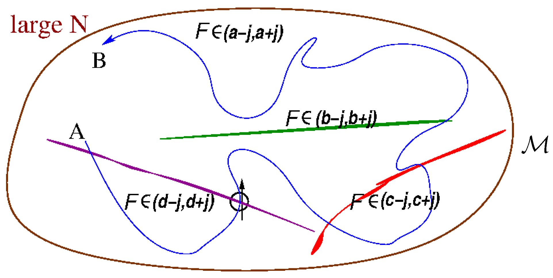
4.1. Time-Dependent Perturbations

Consider a time dependent perturbation of the equations of motion (14) that leads to non-autonomous equations such as:

$$\dot{\Gamma }=\widehat{G}(\Gamma ,t)=G(\Gamma )+p\left(t\right)\text{or}\dot{\Gamma }=\widehat{G}(\Gamma ,t)=p\left(t\right)G(\Gamma ).$$

(27)

On the left hand side, p is a vector field of same dimension as $\mathcal{M}$. On the right hand side, p is a scalar function. If the perturbation is periodic, we may restore the autonomous character of the dynamics introducing new variables φ and θ, that evolve as:

$$\left\{\begin{array}{c}\dot{\theta }=\varphi ,\hfill \\ \dot{\varphi }=-\theta ,\hfill \end{array}\right.$$

(28)

and considering p as function of θ and φ. Let $\tilde{\Gamma }=({\mathbf{q}}_1,\dots ,{\mathbf{q}}_N,{\mathbf{p}}_1,\dots ,{\mathbf{p}}_N,\theta ,\varphi )=(\Gamma ,\theta ,\varphi )$ be one point in the augmented phase space $\tilde{\mathcal{M}}$. We denote by a tilde the counterparts in $\tilde{\mathcal{M}}$ of the quantities previously considered in $\mathcal{M}$:

$$\widetilde{f_0}=\widetilde{f_0}(\Gamma ,\theta ,\varphi )\tilde{\Lambda }=\tilde{\Lambda }(\Gamma ,\theta ,\varphi ){\tilde{\Omega }}^{f_0}={\tilde{\Omega }}^{f_0}(\Gamma ,\theta ,\varphi ).$$

(29)

Then, our perturbation lives on an ellipse, determined by the initial conditions, and the dynamics in $\tilde{\mathcal{M}}$ can be expressed by:

$$\dot{\tilde{\Gamma }}=\tilde{G}(\Gamma ,\theta ,\varphi )=\left(\begin{array}{c}G(\Gamma )+p(\theta ,\varphi )\\ \varphi \\ -\theta \end{array}\right),$$

(30)

or

$$\dot{\tilde{\Gamma }}=\tilde{G}(\Gamma ,\theta ,\varphi )=\left(\begin{array}{c}p(\theta ,\varphi )G(\Gamma )\\ \varphi \\ -\theta \end{array}\right),$$

(31)

where p is a given function of θ and φ. We may endow the ellipse of θ and φ with a uniform probability distribution. Then, the probability density function $\widetilde{f_0}$ in the augmented phase space takes the form:

$$\widetilde{f_0}(\Gamma ,\theta ,\varphi )=\frac{1}{\sigma }{f}_0(\Gamma ),$$

(32)

where σ is the length of the one-dimensional torus. Then, in the case of Equation (30), the new dissipation function takes the form:

$$\begin{array}{cc}\hfill {\tilde{\Omega }}^{f_0}& (\Gamma ,\theta ,\varphi )=-\tilde{\Lambda }(\Gamma ,\theta ,\varphi )-{\displaystyle \frac{d}{dt}}ln{\tilde{f}}_0(\Gamma ,\theta ,\varphi )\hfill \\ & =-\tilde{\Lambda }(\Gamma ,\theta ,\varphi )-{\displaystyle \frac{1}{{\tilde{f}}_0(\Gamma ,\theta ,\varphi )}}\left[\left(G(\Gamma )+p(\theta ,\varphi )\right){\displaystyle \frac{\partial {\tilde{f}}_0(\Gamma ,\theta ,\varphi )}{\partial \Gamma }}+\varphi {\displaystyle \frac{\partial {\tilde{f}}_0(\Gamma ,\theta ,\varphi )}{\partial \theta }}-\theta {\displaystyle \frac{\partial {\tilde{f}}_0(\Gamma ,\theta ,\varphi )}{\partial \varphi }}\right]\hfill \\ & =-{\Lambda }_{old}(\Gamma )-{\displaystyle \frac{1}{f_0(\Gamma )}}\left(G(\Gamma )+p(\theta ,\varphi )\right){\displaystyle \frac{\partial f_0(\Gamma )}{\partial \Gamma }}\hfill \end{array}$$

(33)

because p does not depend on Γ and ${\tilde{f}}_0$ does not depend on θ and φ. Then:

$${\tilde{\Omega }}^{{\tilde{f}}_0}(\Gamma ,\theta ,\varphi )=\underset{\text{old dissipation function}}{\underbrace{{\Omega }_{old}^{f_0}(\Gamma )}}-\underset{\text{additional term}}{\underbrace{p(\theta ,\varphi ){\displaystyle \frac{\partial ln{f}_0}{\partial \Gamma }}(\Gamma )}}.$$

(34)

In the case of Equation (31), we find:

$${\tilde{\Omega }}^{\left(0\right)}(\Gamma ,\theta ,\varphi )=p(\theta ,\varphi )\left(-{\Lambda }_{old}(\Gamma )-G(\Gamma ){\displaystyle \frac{\partial ln{f}_0(\Gamma )}{\partial \Gamma }}\right)=\underset{\text{additional term}}{\underbrace{p(\theta ,\varphi )}}{\tilde{\Omega }}_{old}^{\left(0\right)}(\Gamma ).$$

(35)

The above shows how the dissipation function can be defined in the presence of time dependent perturbations, and how it differs from the unperturbed case. In particular, this is done eliminating the explicit dependence on time, that makes problematic both the notion of TRI and the physical interpretation of the statistical quantities. Once the dissipation function has been re-introduced in such a way that TRI holds in the extended phase space, the results previously obtained for autonomous systems can be transferred to the time dependent case, simply using the modified dissipation function. In particular, observing that θ and φ do not depend on Γ and obey the TRI Equation (28) with an involution operator $\widehat{i}$ such that $\widehat{i}(\theta ,\varphi )=(\theta ,-\varphi )$, we may define $\tilde{i}:\tilde{\mathcal{M}}\to \tilde{\mathcal{M}}$ as:

$$\tilde{i}\tilde{\Gamma }=\tilde{i}\left(\begin{array}{c}\Gamma \\ \theta \\ \varphi \end{array}\right)=\left(\begin{array}{c}i\Gamma \\ \theta \\ -\varphi \end{array}\right).$$

(36)

To understand the conditions under which TRI holds in the perturbed case (30), observe that $p(\theta ,\varphi )$ can be divided in four parts: the vector $p_q(\theta ,\varphi )$ perturbing the evolution of the vector of generalized coordinates, the vector $p_p(\theta ,\varphi )$ perturbing the evolution of the vector of momenta, and two zeros in the position of the variables θ and φ, that are subjected to no perturbation. Then, TRI requires the existence of an involution $\tilde{i}$ such that:

$$\tilde{i}p(\theta ,\varphi )=\tilde{i}\left(\begin{array}{c}{p}_q(\theta ,\varphi )\\ p_p(\theta ,\varphi )\\ 0\\ 0\end{array}\right)=\left(\begin{array}{c}-p_q(\theta ,\varphi )\\ p_p(\theta ,\varphi )\\ 0\\ 0\end{array}\right).$$

(37)

In the case of Equation (31), it suffices instead to have an even function p:

$$p(\theta ,-\varphi )=p(\theta ,\varphi ).$$

(38)

This approach may be extended to more general time dependent perturbations, since any perturbation can be thought to be periodic of period T, if T is conveniently larger than the observation times [28]. For instance, any periodic function $p\in {\mathcal{L}}^2[0,T]$ can be expanded in Fourier components:

$$p\left(t\right)={\displaystyle \sum _{n=-\infty }^{\infty }}{V}_n{e}^{i{\omega }_{n}t},$$

(39)

with ${\omega }_n=2\pi n/T$, and one may eliminate t introducing the representation:

$$p\left(t\right)=p(\theta ,\varphi )={\displaystyle \sum _{n=-\infty }^{\infty }}{V}_n{p}_n(\theta ,\varphi ),$$

(40)

where with a slight abuse of notation, θ and φ replace t and obey:

$$\left\{\begin{array}{c}\dot{\theta }=\varphi ,\hfill \\ \dot{\varphi }=-{\omega }^2\theta ,\hfill \end{array}\right.\text{with}{\omega }^2={\left(\frac{2\pi }{T}\right)}^2,$$

(41)

while the n-th Fourier basis element has been replaced by:

$$p_n={\left(\theta -i\frac{\varphi }{\omega }\right)}^n,n\in \mathbb{Z}.$$

(42)

Then, the equations of motion in the extended phase space $\tilde{\mathcal{M}}$ can be written as:

$$\left(\begin{array}{c}{\dot{\tilde{\Gamma }}}_1\\ {\dot{\tilde{\Gamma }}}_2\\ ⋮\\ {\dot{\tilde{\Gamma }}}_{2N}\\ \dot{\theta }\\ \dot{\varphi }\end{array}\right)=\left(\begin{array}{c}G\left({\Gamma }_1\right)+{\sum }_{n=-\infty }^{\infty }{V}_{n1}{\left(\theta -i\frac{\varphi }{\omega }\right)}^n\\ G\left({\Gamma }_2\right)+{\sum }_{n=-\infty }^{\infty }{V}_{n2}{\left(\theta -i\frac{\varphi }{\omega }\right)}^n\\ ⋮\\ G\left({\Gamma }_{2N}\right)+{\sum }_{n=-\infty }^{\infty }{V}_{n2N}{\left(\theta -i\frac{\varphi }{\omega }\right)}^n\\ \varphi \\ -{\omega }^2\theta \end{array}\right),$$

(43)

while the dissipation function takes the form:

$$\begin{array}{}(44)& \hfill {\tilde{\Omega }}^{f_0}& (\Gamma ,\theta ,\varphi )=-{\Lambda }_{old}(\Gamma )-{\displaystyle \sum _{k=0}^{2N}}{G}_k(\Gamma )\frac{\partial ln{f}_0(\Gamma )}{\partial {\Gamma }_k}-{\displaystyle \sum _{k=0}^{2N}\sum _{n=-\infty }^{\infty }}{V}_{nk}{\left(\theta -i\frac{\varphi }{\omega }\right)}^n\frac{\partial ln{f}_0(\Gamma )}{\partial {\Gamma }_k},\hfill (45)& & =\underset{\text{old dissipation function}}{\underbrace{{\Omega }_{old}^{f_0}(\Gamma )}}-\underset{\text{additional term}}{\underbrace{{\displaystyle \sum _{k=0}^{2N}\sum _{n=-\infty }^{\infty }}{V}_{nk}{\left(\theta -i\frac{\varphi }{\omega }\right)}^n\frac{\partial ln{f}_0(\Gamma )}{\partial {\Gamma }_k}}}.\hfill \end{array}$$

This expression is more general than Equation (34) since it holds for all ${\mathcal{L}}^2[0,T]$ perturbations given any observation interval $[0,T]$.

It appears that, in general, TRI may be violated because of the time dependent perturbation p. If that is the case, some of the results strictly related to TRI may fail, but a number of other results implied by the existence of a dissipation function still hold. Indeed, even the FR continues to hold in various cases in which TRI is absent, cf. Ref. [29]. Moreover, the end of Section 3 shows that, in many situations, TRI is not obvious but still present. The different situations must be assessed case by case. Keeping this in mind, in the following, we do not distinguish the autonomous from the non-autonomous cases.

4.2. Fluctuation Relations: Symmetry in Dissipative Dynamics

While the main purpose of the dissipation function is to describe the response to perturbations, and the relaxation of dynamical systems, it has been introduced to express one symmetry of TRI dissipative dynamics: the FR.

Let $\mathcal{O}$ be a physical observable that is odd with respect to the time reversal operator i, $\mathcal{O}\left(ix\right)=-\mathcal{O}\left(x\right)$. For $\delta >0$, introduce the interval ${\left(A\right)}_{\delta }=(A-\delta ,A+\delta )$, and for a system with initial probability density $f_0$, consider the probability that the average of $\mathcal{O}$ in the time interval $(0,\tau )$, ${\overline{\mathcal{O}}}_{0,\tau }$ say, belongs to ${\left(A\right)}_{\delta }$. By definition, this probability is given by ${\int }_{{{\overline{\mathcal{O}}}_{0,\tau }|}_{{\left(A\right)}_{\delta }}}{f}_0(\Gamma )d\Gamma$, where ${{\overline{\mathcal{O}}}_{0,\tau }|}_{{\left(A\right)}_{\delta }}$ is the set of phase points for which ${\overline{\mathcal{O}}}_{0,\tau }$ lies in ${\left(A\right)}_{\delta }$. Then, we have:

$$\frac{{\mu }_0\left({{\overline{\mathcal{O}}}_{0,\tau }|}_{{(-A)}_{\delta }}\right)}{{\mu }_0\left({{\overline{\mathcal{O}}}_{0,\tau }|}_{{\left(A\right)}_{\delta }}\right)}=\frac{{\int }_{{{\overline{\mathcal{O}}}_{0,\tau }|}_{{(-A)}_{\delta }}}{f}_0(\Gamma )d\Gamma }{{\int }_{{{\overline{\mathcal{O}}}_{0,\tau }|}_{{\left(A\right)}_{\delta }}}{f}_0(\Gamma )d\Gamma },$$

(46)

which can be computed observing that

$${{\overline{\mathcal{O}}}_{0,\tau }|}_{{(-A)}_{\delta }}={i{S}^{\tau }{\overline{\mathcal{O}}}_{0,\tau }|}_{{\left(A\right)}_{\delta }}.$$

(47)

Hence, introducing the coordinate transformation $\Gamma =i{S}^{\tau }x$, whose Jacobian is $\left|\frac{\partial \Gamma }{\partial x}\right|=exp\left\{{\Lambda }_{0,\tau }\left(x\right)\right\}$, cf. Ref. [23] Equation (46) becomes:

Transient $\mathcal{O}$-FR:

$$\begin{array}{c}\hfill \frac{{\mu }_0\left({\overline{\mathcal{O}}}_{0,\tau }{|}_{{(-A)}_{\delta }}\right)}{{\mu }_0\left({\overline{\mathcal{O}}}_{0,\tau }{|}_{{\left(A\right)}_{\delta }}\right)}=\frac{{\int }_{{\overline{\mathcal{O}}}_{0,\tau }{|}_{{\left(A\right)}_{\delta }}}{f}_0\left(S^{\tau }X\right)e^{{\Lambda }_{0,\tau }\left(X\right)}\mathrm{d}X}{{\int }_{{\overline{\mathcal{O}}}_{0,\tau }{|}_{{\left(A\right)}_{\delta }}}{f}_0(\Gamma )\mathrm{d}\Gamma }:={〈e^{-{\Omega }_{0,\tau }^{\left(0\right)}}〉}_{{\overline{\mathcal{O}}}_{0,\tau }\in {\left(A\right)}_{\delta }}^{\left(0\right)},\end{array}$$

(48)

where the last average is computed with respect to ${\mu }_0$ over the set of initial conditions such that ${\overline{\mathcal{O}}}_{0,\tau }(\Gamma )\in {\left(A\right)}_{\delta }$, and we use the following definitions for the dissipation function:

$${\overline{\Omega }}_{t,t+\tau }^{\left(0\right)}(\Gamma )=\frac{1}{\tau }{\Omega }_{t,t+\tau }^{\left(0\right)}=\frac{1}{\tau }ln\frac{f_0(S^t\Gamma )}{f_0(S^{t+\tau }\Gamma )}-{\overline{\Lambda }}_{t,t+\tau }(\Gamma ),$$

(49)

and we have assumed $f_0$ to be even under i, which means that $f_0$ could be an equilibrium probability density. At the same time, the phase space expansion rate Λ is odd with respect to i. If $\mathcal{O}={\Omega }^{\left(0\right)}$, we obtain:

Transient Ω-FR:

$$\frac{{\mu }_0\left({\overline{\Omega }}_{0,\tau }^{\left(0\right)}{|}_{{(-A)}_{\delta }}\right)}{{\mu }_0\left({\overline{\Omega }}_{0,\tau }^{\left(0\right)}{|}_{{\left(A\right)}_{\delta }}\right)}={〈exp\left(-{\Omega }_{0,\tau }^{\left(0\right)}\right)〉}_{{\overline{\Omega }}_{0,\tau }^{\left(0\right)}\in {\left(A\right)}_{\delta }}^{\left(0\right)}=e^{-[A+ϵ(\delta ,A,\tau )]\tau },$$

(50)

where the magnitude of $ϵ(\delta ,A,\tau )$ is at most δ, because the average in Equation (50) is computed over the initial conditions, which lead to a value for ${\overline{\Omega }}_{0,\tau }^{\left(0\right)}$ within a distance δ from A.

Remarkably, the only conditions for these results are that the system starts from a state defined by an even $f_0$, and that its dynamics obeys TRI. These transient relations describe the statistics of repeated measurements of the observable $\mathcal{O}$ in a time τ, starting in the same equilibrium state followed by some work for a time τ. This allows us to gain information on the initial equilibrium state, thanks to some nonequilibrium process. In this sense, transient FRs close the circle with the fluctuation-dissipation relations which, on the contrary, get information on nonequilibrium properties from equilibrium experiments.

For the behaviour in a steady-state, one may consider the following expression:

$$\frac{{\mu }_0\left({\overline{\mathcal{O}}}_{t,t+\tau }{|}_{{(-A)}_{\delta }}\right)}{{\mu }_0\left({\overline{\mathcal{O}}}_{t,t+\tau }{|}_{{\left(A\right)}_{\delta }}\right)}=\frac{{\int }_{{\overline{\mathcal{O}}}_{t,t+\tau }{|}_{{(-A)}_{\delta }}}{f}_0(\Gamma )d\Gamma }{{\int }_{{\overline{\mathcal{O}}}_{t,t+\tau }{|}_{{\left(A\right)}_{\delta }}}{f}_0(\Gamma )d\Gamma }.$$

(51)

in the $t\to \infty$ limit. For any finite t, one has:

$${\overline{\mathcal{O}}}_{t,t+\tau }{{|}_{{(-A)}_{\delta }}=\mathcal{I}{S}^{2t+\tau }{\overline{\mathcal{O}}}_{t,t+\tau }|}_{{\left(A\right)}_{\delta }},$$

(52)

which reduces to the previous expression (47) for $t=0$. Therefore, by introducing $X\in \mathcal{M}$ so that $\Gamma =i{S}^{2t+\tau }X$ and by using the parity of $f_0$ with respect to TRI, we obtain:

$$\begin{array}{ccc}\hfill {\int }_{{\overline{\mathcal{O}}}_{t,t+\tau }{|}_{{(-A)}_{\delta }}}{f}_0(\Gamma )\mathrm{d}\Gamma & =& {\int }_{{\overline{\mathcal{O}}}_{t,t+\tau }{|}_{{\left(A\right)}_{\delta }}}{f}_0\left(X\right)e^{-{\Omega }_{0,2t+\tau }\left(X\right)}\mathrm{d}X,.\hfill \end{array}$$

(53)

Substituting Equation (53) in Equation (51), the result is:

$$\frac{{\mu }_0\left({\overline{\mathcal{O}}}_{t,t+\tau }{|}_{{(-A)}_{\delta }}\right)}{{\mu }_0\left({\overline{\mathcal{O}}}_{t,t+\tau }{|}_{{\left(A\right)}_{\delta }}\right)}={〈exp\left(-{\Omega }_{0,2t+\tau }^{\left(0\right)}\right)〉}_{{\overline{\mathcal{O}}}_{t,t+\tau }\in {\left(A\right)}_{\delta }}^{\left(0\right)},$$

(54)

where the right-hand side is an average over the phase space trajectory segments for which ${\overline{\mathcal{O}}}_{t,t+\tau }(\Gamma )$ is close to A.

This is still a transient identity, fundamentally based only TRI for $f_0$. We may now use the generalized Liouville equation for the conservation of probability to replace the initial distribution of density $f_0$ in (54) with the distribution ${\mu }_t$ of density $f_t$, which is reached by evolving $f_0$ for a time t:

$${\mu }_t\left(S^{t}E\right)={\mu }_0\left(E\right)\text{i.e.,}{\int }_{S^{t}E}{f}_t\left(X\right)dX={\int }_E{f}_0\left(X\right)dX$$

$$\Rightarrow {\mu }_0\left({\overline{\mathcal{O}}}_{t,t+\tau }{|}_{{\left(A\right)}_{\delta }}\right)={\mu }_t\left(S^t{\overline{\mathcal{O}}}_{t,t+\tau }{|}_{{\left(A\right)}_{\delta }}\right)={\mu }_t\left({\overline{\mathcal{O}}}_{0,\tau }{|}_{{\left(A\right)}_{\delta }}\right)..$$

(55)

By combining Equations (54) and (55), we get the following relation:

$$\frac{{\mu }_t\left({\overline{\mathcal{O}}}_{0,\tau }{|}_{{(-A)}_{\delta }}\right)}{{\mu }_t\left({\overline{\mathcal{O}}}_{0,\tau }{|}_{{\left(A\right)}_{\delta }}\right)}={〈exp\left(-{\Omega }_{0,2t+\tau }^{\left(0\right)}\right)〉}_{{\overline{\mathcal{O}}}_{t,t+\tau }\in {\left(A\right)}_{\delta }}^{\left(0\right)},$$

(56)

which, in the case $\mathcal{O}={\Omega }^{\left(0\right)}$, eventually leads to:

$$\begin{array}{}(57)& \hfill \frac{{\mu }_t\left({\overline{\Omega }}_{0,\tau }^{\left(0\right)}{|}_{{(-A)}_{\delta }}\right)}{{\mu }_t\left({\overline{\Omega }}_{0,\tau }^{\left(0\right)}{|}_{{\left(A\right)}_{\delta }}\right)}& =& {〈e^{-{\Omega }_{0,t}^{\left(0\right)}}{e}^{-{\Omega }_{t,t+\tau }^{\left(0\right)}}{e}^{-{\Omega }_{t+\tau ,2t+\tau }^{\left(0\right)}}〉}_{{\overline{\Omega }}_{t,t+\tau }^{\left(0\right)}\in {\left(A\right)}_{\delta }}^{\left(0\right)},\hfill (58)& & =& e^{-\left[A+ϵ(\delta ,t,A,\tau )\right]\tau }{〈e^{-{\Omega }_{0,t}}{e}^{-{\Omega }_{t+\tau ,2t+\tau }}〉}_{{\overline{\Omega }}_{t,t+\tau }^{\left(0\right)}\in {\left(A\right)}_{\delta }}^{\left(0\right)},\hfill \end{array}$$

where only part of the integral on the right-hand side is constrained. This relation is exact and holds for all values of t, τ and all pairs of A and $-A$. Moreover, the probability measures are no longer computed with respect to the initial density $f_0$, like in the previous transient FR, but they refer to the density $f_t$ that may eventually approach in time the steady-state distribution.

The existence of a steady-state FR implies that the expression (58) tends to a given value as $t\to \infty$, while the ratio of probabilities in expression (57) does. Assuming that such a steady-state FR holds, we may now investigate which conditions are necessarily verified.

4.3. t-Mixing and Irreversibility

Let us rewrite Equation (58) in a more convenient way as follows:

$$\frac{1}{\tau }ln\frac{{\mu }_t\left({\overline{\Omega }}_{0,\tau }^{\left(0\right)}{|}_{{\left(A\right)}_{\delta }}\right)}{{\mu }_t\left({\overline{\Omega }}_{0,\tau }^{\left(0\right)}{|}_{{(-A)}_{\delta }}\right)}=A+ϵ(\delta ,t,A,\tau )-\frac{1}{\tau }ln{\mathcal{C}}_0(A,\delta ,t,\tau ),$$

(59)

where we have introduced a new symbol ${\mathcal{C}}_0$ to stress its role in the following:

$${\mathcal{C}}_0(A,\delta ,t,\tau ):={〈e^{-{\Omega }_{0,t}^{\left(0\right)}-{\Omega }_{t+\tau ,2t+\tau }^{\left(0\right)}}〉}_{{\overline{\Omega }}_{t,t+\tau }^{\left(0\right)}\in {\left(A\right)}_{\delta }}^{\left(0\right)}={〈{\mathcal{Q}}_t\left({\mathcal{Q}}_t\circ S^{t+\tau }\right)〉}_{{\overline{\Omega }}_{t,t+\tau }^{\left(0\right)}\in {\left(A\right)}_{\delta }}^{\left(0\right)}$$

(60)

as a kind of auto-correlation function for the following observable:

$${\mathcal{Q}}_t(\Gamma ):=exp\left[-{\int }_0^t{\Omega }^{\left(0\right)}(S^u\Gamma )\mathrm{d}u\right].$$

(61)

Note that, in Equation (60), the average is computed with respect to the initial probability distribution ${\mu }_0$.

Suppose now to take the $t\to \infty$ limit at fixed A, δ, τ of Equation (59). If the logarithm of ${\mathcal{C}}_0$ diverges, one of the probabilities of the left-hand side of (59) goes to zero, which means that either A or $-A$ are not observable at the steady state, i.e., when the probability distribution is ${\mu }_{\infty }$. Clearly, if no pair $(A,-A)$ is observable, the steady-state FR is of no interest. On the contrary, if observable pairs $(A,-A)$ do exist, it means that, for such values, a steady-state FR in fact holds, i.e., the ratio of the probabilities to observe such values with respect to ${\mu }_{\infty }$ must satisfy the following inequalities, for any $\delta >0$:

$$A-\delta \le \frac{1}{\tau }ln\frac{{\mu }_{\infty }\left({\overline{\Omega }}_{0,\tau }^{\left(0\right)}{|}_{{\left(A\right)}_{\delta }}\right)}{{\mu }_{\infty }\left({\overline{\Omega }}_{0,\tau }^{\left(0\right)}{|}_{{(-A)}_{\delta }}\right)}\le A+\delta .$$

(62)

The relation (62) evidently implies that the $t\to \infty$ limit of the term containing the auto-correlation function ${\mathcal{C}}_0$ is negligible. Then, relation (62) follows in the $\tau \to \infty$ limit, if ${\mathcal{C}}_0$ does not grow exponentially fast with τ. This points out a necessary condition for the steady-state FR to hold for a pair $(A,-A)$, i.e., the decay in the auto-correlation with respect to the initial (non-invariant) distribution of the variable defined by Equation (61). Thanks to that, Equation (60) can be factorized as follows:

$${〈e^{-{\Omega }_{0,t}^{\left(0\right)}-{\Omega }_{t+\tau ,2t+\tau }^{\left(0\right)}}〉}^{\left(0\right)}={〈e^{-{\Omega }_{0,t}^{\left(0\right)}}〉}^{\left(0\right)}{〈e^{-{\Omega }_{t+\tau ,2t+\tau }^{\left(0\right)}}〉}^{\left(0\right)}.$$

(63)

Equation (63) is one instance of the following property, which we call weak t-mixing:

$$\underset{t\to \infty }{lim}\left[{〈\mathcal{Q}\left(\mathcal{O}\circ S^t\right)〉}^{\left(0\right)}-{〈\mathcal{Q}〉}^{\left(0\right)}{〈\mathcal{O}\circ S^t〉}^{\left(0\right)}\right]=0.$$

(64)

The name derives from the fact that this property is a form of mixing, but it concerns the probability measure associated with the transient initial state.

Taking $\mathcal{Q}={\Omega }^{\left(0\right)}$ in Equation (64), and recalling that ${\langle {\Omega }^{\left(0\right)}\rangle }^{\left(0\right)}=0$ because ${\Omega }^{\left(0\right)}$ is odd for even $f_0$, Equation (64) amounts to what we call weak Ωt-mixing condition:

$$\underset{t\to \infty }{lim}{〈{\Omega }^{\left(0\right)}\left(\mathcal{O}\circ S^t\right)〉}^{\left(0\right)}=0.$$

(65)

Then, the response formula in Equation (24) can be written in asymptotic form as:

$${\langle \mathcal{O}\rangle }^{\infty }={\langle \mathcal{O}\rangle }^{\left(0\right)}+{\int }_0^{\infty }\mathrm{d}s{〈{\Omega }^{\left(0\right)}\left(\mathcal{O}\circ S^s\right)〉}^{\left(0\right)},$$

(66)

which is the response of the initial ensemble to some perturbation codified within the evolution operator $S^t$. We call Ωt-mixing the condition under which the integral in (66) exists. This is the necessary and sufficient condition for an ensemble of systems to reach steady-state after the driving. Equation (66) is exact, unlike the Green–Kubo linear response formula, which is first order in the perturbation.

Note that ensemble results are the standard results in response theory because the behaviour of single macroscopic systems has been hard to treat so far. Still, in experiments as well as in every day life, we observe the evolution of single systems, rather than that of large collections of identical objects. Ensemble results are accepted under the assumption that the evolution of a single system would not differ significantly from the average one, which is then called typical behaviour. Typical is the behaviour shared by the vast majority of systems. For Hamiltonian macroscopic systems, this is then the behaviour of probability 1, with respect to the invariant, equilibrium distribution, i.e., the counterpart of “counting” in continuous spaces.

In the case of dissipative dynamics, this is not possible because the corresponding invariant measures are singular with respect to the Lebesgue measure, and they attribute probability 1 to sets of zero phase space volume, i.e. to sets that are negligible from the counting standpoint. Nevertheless, the weak t-mixing condition allows us to make some progress in this direction. For any observable $\mathcal{O}$ and any integer n, let

$$E_n^{\mathcal{O},\delta }=\left\{\Gamma :\overline{\mathcal{O}}(\Gamma )=\underset{T\to \infty }{lim}\frac{1}{T}{\int }_0^T\mathcal{O}(S^t\Gamma )\mathrm{d}t\in [n\delta ,(n+1)\delta )\right\}$$

(67)

be the set of initial conditions $\Gamma \in \mathcal{M}$ such that a measurement that lasts very many microscopic times yields a given value within a tolerance δ. By construction, these sets are disjoint and invariant, i.e., a trajectory starting in one set remains inside it forever:

$$S^{-t}{E}_n^{\mathcal{O},\delta }=E_n^{\mathcal{O},\delta }.$$

Now suppose that the time-average $\overline{\mathcal{O}}(\Gamma )$ exists for almost all Γ, in the sense of the Lebesgue measure. This is a delicate assumption because, apart from some idealized situation, one can prove existence of time averages only for ${\mu }_{\infty }$-almost all phases, where ${\mu }_{\infty }$ is the steady-state probability distribution. This is not the desired case, since “almost all” could mean a set of vanishing volume in $\mathcal{M}$. At the same time, it is rather common for systems of physical interest that $\overline{\mathcal{O}}(\Gamma )$ exists almost everywhere in the sense of phase space volumes. Therefore, we assume this to be the case. We may then write:

$${\bigcup }_{n\in \mathbb{Z}}{E}_n^{\mathcal{O},\delta }=\mathcal{M},\text{hence}{\mu }_0\left({\bigcup }_{n\in \mathbb{Z}}{E}_n^{\mathcal{O},\delta }\right)=1.$$

(68)

Let us now introduce the characteristic function ${\chi }_n^{\mathcal{O},\delta }$ of the sets $E_n^{\mathcal{O},\delta }$ defined as:

$${{\chi }_E}^{(\Gamma )}=\left\{\begin{array}{cc}1\hfill & \text{if} \Gamma \in E,\hfill \\ 0\hfill & \text{if} \Gamma \notin E.\hfill \end{array}\right.$$

If we assume that the characteristic functions verify weak t-mixing, we have:

$${\mu }_0\left(E_n^{\mathcal{O},\delta }\cap S^{-t}{E}_n^{\mathcal{O},\delta }\right)-{\mu }_0\left(S^{-t}{E}_n^{\mathcal{O},\delta }\right){\mu }_0\left(E_n^{\mathcal{O},\delta }\right)⟶0$$

(69)

in the $t\to \infty$ limit. Because of the invariance of $E_n^{\mathcal{O},\delta }$ under the dynamics, this yields:

$${\mu }_0\left(E_n^{\mathcal{O},\delta }\right)-{\mu }_0{\left(E_n^{\mathcal{O},\delta }\right)}^2⟶0\text{for} t\to \infty ,$$

and, because there is no time dependence in this equation, one concludes

$${\mu }_0\left(E_n^{\mathcal{O},\delta }\right)=0 \text{or} 1.$$

(70)

Since ${\mu }_0$ can be taken to be absolutely continuous with respect to the Lebesgue measure, and to be supported on all $\mathcal{M}$, this equality means that almost all time averages, with the exception of a set of zero volume, take the same value with an arbitrarily small error δ. If we express relaxation towards a steady state in terms of the behaviour of observables of a system, which is indeed the way we establish equilibrium, Equation (70) states that: under weak t-mixing, single systems relax in a typical fashion, where typical is intended in the sense of counting even for dissipative dyamics.

5. Conclusions

In this contribution we have outlined a physical interpretation of the problem of macroscopic irreversibility, the temporal symmetry breaking of our daily life space and time scales, for relaxation of TRI dissipative systems, such as those of NEMD.

In the case of conservative dynamics, the standard approach is represented by Boltzmann’s argument. This argument rests on the notion of typicality, which implies that a system starting in a non-equilibrium state with dynamics exploring the phase space without constraints irreversibly enters its proper equilibrium state. In our view, one difficulty of this approach is that it subordinates the irreversibility that we experience on our space and time scales to the evolution of the whole universe and its initial conditions: the “past hypothesis”. Although the argument is fascinating and quite compelling within a given rational framework, it embeds in a single theory such remote scales as the microscopic, the macroscopic (or thermodynamic), and the cosmological scales. The purpose of explanation may therefore be better served by an approach that appears less fundamental but avoids numerous steps not amenable to experimental tests.

Other recent studies [30] have shown that, at least for simple Newtonian N–body systems, a gravitational arrow of time seems to naturally arise out of simple physical laws without the need for special initial conditions, in contrast with the standard Boltzmann’s view. The approach of Ref. [30] has been, however, criticized [31]. Former approaches, such as Prigogine’s recourse to microscopically irreversible dynamics, also appear unnecessary, as we have no evidence of this lack of reversibility at the atomic/molecular scale, despite violations of the time parity being observed in high energy physics.

Our approach is based on the theory of TRI dissipative dynamical systems, which successfully describe transport properties of nonequilibrium systems, focusing on the molecular level of description. Indeed, one may argue that dissipation phenomena fit human space and time scales much better than the universe as a whole does. The key hypothesis of this model is the microscopic time reversal invariance of the dynamics.

The technical tool that we have used to achieve our result is the dissipation function:

$${\Omega }^{\left(0\right)}=-G·{\partial }_{\Gamma }ln{f}^{\left(0\right)}-\Lambda ,$$

which we considered as a nonequilibrium thermodynamic potential, driving the relaxation of an ensemble of systems arbitrarly far from equilibrium. We extended the corresponding formalism to the case of time-dependent perturbations acting on the system. Furthermore, we have illustrated how weak t-mixing turns ensemble results into single system ones. Under the assumption of the existence of time averages for ${\mu }_0$—almost every $\Gamma \in \mathcal{M}$—we have thus extended the “counting” argument even to TRI dissipative systems.

For a single system, arbitrarly far from equilibrium, we have proved that the condition to observe irreversible relaxation to a nonequilibrium steady state is the decay of auto-correlation of the dissipation function.

Loss of memory again is connected with the presence of different time scales, i.e., the fact that any measurement of a system takes a certain characteristic time to be made, which is very long compared to the microscopic characteristic times. For future investigations, it will be important to understand the role played by the system size N in the t-mixing conditions.

References

1. Cohen, L. The history of noise. IEEE Signal Process. Mag. 2005, 22, 20–45. [Google Scholar] [CrossRef]
2. Cercignani, C. The Boltzmann Equation and Its Applications; Spriger-Verlag: Berlin, Germany, 1987. [Google Scholar]
3. Lebowitz, J. Boltzmann’s Entropy and Time’s Arrow. Phys. Today 1993, 46, 32–38. [Google Scholar] [CrossRef]
4. Hoover, W.G.; Posch, H.; Holian, B.L. Is Boltzmann Entropy Time’s Arrow’s Archer? Phys. Today 1994, 47. [Google Scholar] [CrossRef]
5. Goldstein, T. Typicality and Notions of Probability in Physics. In Probability in Physics; Ben-Menahem, Y., Hemmo, M., Eds.; Springer-Verlag: Berlin, Germany, 2012. [Google Scholar]
6. Khinchin, A. Mathematical Foundations of Statistical Mechanics; Dover Publications: New York, NY, USA, 1949. [Google Scholar]
7. Cover, T.M.; Thomas, J.A. Elements of Information Theory; Wiley: New York, NY, USA, 1991. [Google Scholar]
8. Castiglione, P.; Falcioni, M.; Lesne, A.; Vulpiani, A. Chaos and Coarse Graining in Statistical Mechanics; Cambridge University Press: Cambridge, UK, 2008. [Google Scholar]
9. Cerino, L.; Cecconi, F.; Cencini, M.; Vulpiani, A. The role of the number of degrees of freedom and chaos in macroscopic irreversibility. Physica A 2016, 442, 486–497. [Google Scholar] [CrossRef]
10. Pitowsky, I. Typicality and the Role of the Lebesgue Measure in Statistical Mechanics. In Probability in Physics; Ben-Menahem, Y., Hemmo, M., Eds.; Springer-Verlag: Berlin, Germany, 2012. [Google Scholar]
11. Penrose, R. The Road to Reality: A Complete Guide to the Laws of the Universe; Jonathan Cape: London, UK, 2004. [Google Scholar]
12. Albert, D.Z. Time and Chance; Harvard University Press: Cambridge, MA, USA, 2000. [Google Scholar]
13. Evans, D.J.; Morriss, G.P. Statistical Mechanics of Nonequilibrium Liquids; Cambridge University Press: Cambridge, UK, 2008. [Google Scholar]
14. Chibbaro, S.; Rondoni, L.; Vulpiani, A. Reductionism, Emergence and Levels of Reality. The Importance of Being Borderline; Springer: New York, NY, USA, 2014. [Google Scholar]
15. Jepps, O.; Rondoni, L. Deterministic thermostats, theories of nonequilibrium systems and parallels with the ergodic condition. J. Phys. A Math. Theor. 2010, 43, 1–42. [Google Scholar] [CrossRef]
16. Evans, D.J.; Cohen, E.G.D.; Morriss, G.P. Probability of second law violations in shearing steady flows. Phys. Rev. Lett. 1993, 71, 2401. [Google Scholar] [CrossRef] [PubMed]
17. Bonaldi, M.; Conti, L.; De Gregorio, P.; Rondoni, L.; Vedovato, G.; Vinante, A.; Bignotto, M.; Cerdonio, M.; Falferi, P.; Liguori, N.; et al. Nonequilibrium Steady-State Fluctuations in Actively Cooled Resonators. Phys. Rev. Lett. 2009, 103, 010601. [Google Scholar] [CrossRef] [PubMed]
18. Conti, L.; Lazzaro, C.; Karapetyan, G.; Bonaldi, M.; Pegoraro, M.; Thakur, R.-K.; De Gregorio, P.; Rondoni, L. Thermal noise of mechanical oscillators in steady states with a heat flux. Phys. Rev. E 2014, 90, 032119. [Google Scholar] [CrossRef] [PubMed]
19. Bonella, S.; Ciccotti, G.; Rondoni, L. Time reversal symmetry in time-dependent correlation functions for systems in a constant magnetic field. EPL 2014, 108, 60004. [Google Scholar] [CrossRef]
20. De Grood, S.R.; Mazur, P. Non-Equilibrium Thermodynamics; Dover Publications: New York, NY, USA, 2011. [Google Scholar]
21. Gabrielli, D.; Jona-Lasinio, G.; Landim, C. Onsager Symmetry from Microscopic TP Invariance. J. Stat. Phys. 1999, 96, 639–652. [Google Scholar] [CrossRef]
22. Gaspard, P. Multivariate fluctuation relations for currents. New J. Phys. 2013, 15, 115014. [Google Scholar] [CrossRef]
23. Searles, D.J.; Rondoni, L.; Evans, D.J. The steady state fluctuation relation for the dissipation function. J. Stat. Phys. 2007, 128, 1337–1363. [Google Scholar] [CrossRef]
24. Jepps, O.G.; Rondoni, L. A dynamical-systems interpretation of the dissipation function, T-mixing and their relation to thermodynamic relaxation. J. Phys. A 2016, 49, 154002. [Google Scholar] [CrossRef]
25. Rondoni, L.; Evans, D.J.; Searles, D.J.; Williams, S.R. On typicality in nonequilibrium steady states. J. Stat. Phys. 2016, in press. [Google Scholar]
26. Evans, D.J.; Searles, D.J. The Fluctuation Theorem. Adv. Phys. 2002, 51, 1529. [Google Scholar] [CrossRef]
27. Evans, D.J.; Searles, D.J.; Williams, S.R. On the Fluctuation Theorem for the Dissipation Function and Its Connection with Response Theory. J. Chem. Phys. 2008, 128, 014504. [Google Scholar] [CrossRef] [PubMed]
28. Kubo, R.; Toda, M.; Hashitsume, N. Statistical Physics II, Nonequilibrium Statistical Mechanics; Springer Verlag: Heidelberg, Germany, 1985. [Google Scholar]
29. Colangeli, M.; Rondoni, L. Equilibrium, fluctuation relations and transport for irreversible deterministic dynamics. Physica D 2012, 241, 681–691. [Google Scholar] [CrossRef]
30. Barbour, J.; Koslowski, T.; Mercati, F. Identification of a Gravitational Arrow of Time. Phys. Rev. Lett. 2014, 113, 181101. [Google Scholar] [CrossRef] [PubMed]
31. Goldstein, S.; Tumulka, R.; Zanghí, N. Is the Hypothesis about a Low Entropy Initial State of the Universe Necessary for Explaining the Arrow of Time? 2016; arXiv:1602.05601. [Google Scholar]
Figure 1. The phase space M is imaginatively represented by an oblong figure. Let F be a phase variable on M . For one many particles system, the region corresponding to the equilibrium value a of F, measured with accuracy j, is by far the largest region of M : most of M is occupied by the phases Γ such that F ( Γ ) ( a j , a + j ) (white region). The regions corresponding to values b , c , d , a are represented by thin strips, that are much smaller than the equilibrium region. A trajectory γ in M is represented by a blue line, with an arrow at its upper end (B), indicating the direction of time. Let the (purely conventional) initial condition Γ of γ lie in the purple strip within the black ring, where γ is oriented upward. Evolving in the direction from A to B, the Γ in the nonequilibrium region (low entropy state), rapidly reaches the equilibrium much larger region (highest entropy state), and remains there, apart from fleeting deviations, when it enters the slim colored strips. Tracing γ backward in time means going in the direction opposite to the arrows (direction from B to A); even in this backward direction one rapidly moves out of whatever low entropy colored region, and falls in a state of higher entropy. For the Hamiltonian description, Ref. [3] states that both forward and backward evolutions out of any colored strip go from low to high entropy states (see also Reference [2] Section 5.5 and Reference [11] Section 27.5).
Symmetry 08 00073 g001