
Iterative Speedup by Utilizing Symmetric Data in Pricing Options with Two Risky Assets

Abstract
:1. Introduction
2. Nomenclature
3. Implicit OSM
- Step (1)
- Find the solution at , by discretizing the equation with the given :
- Step (2)
- Find the solution at , by discretizing the equation with the solution found in Step (1) as the given condition:
4. Iterative Crank–Nicolson Method
- Step (1)
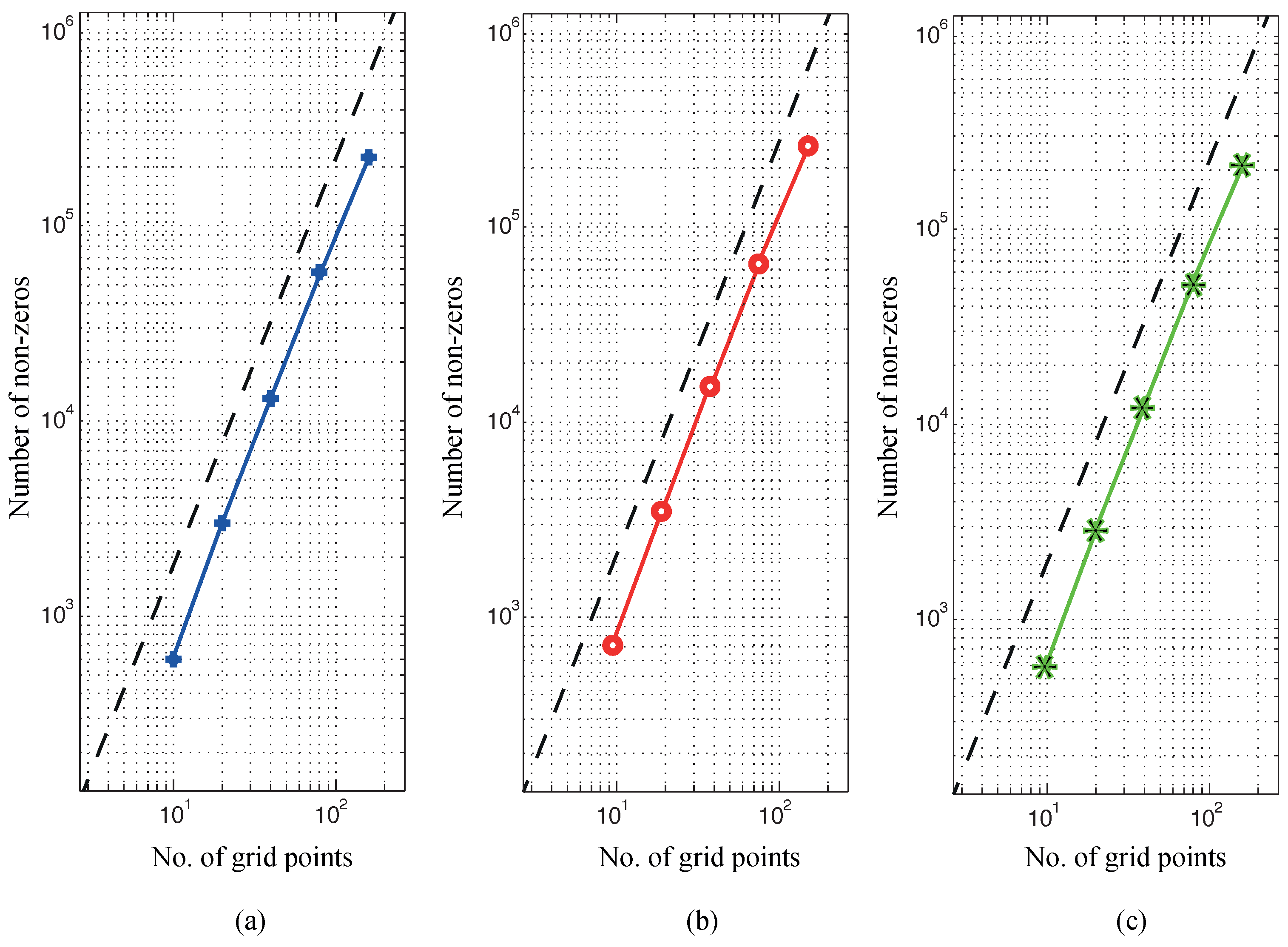
- Get a linear system by discretizing Equation (1) with the Crank–Nicolson scheme. The following equation is matrix-vector form of the Equation (15) :whereNote that the data, and , grows quadratically in terms of the grid points. In addition, the system in Equation (16) is non-symmetric.
- Step (2)
- Apply appropriate boundary conditions to the and . Depending on the option type, the boundary condition is either given as a linear boundary condition on the truncated interface or an essential boundary condition where the price of the option is zero. We denote the boundary condition imposed system as follows:
- Step (3)
- Symmetrize the system given in Equation (19) as follows:where is the transpose of
- Step (4)
- Create preconditioned matrix with using incomplete LU factorization (where LU stands for lower and upper triangular matrix). The choice of the preconditioner is more important than the choice of the Krylov iterative method such as GMRES [14,15]. The effectiveness of preconditioner created by incomplete LU factorization is measured by how well approximates the .
- Step (5)
- Solve Equation (20) repetitively using GMRES with the preconditioner and the previous solution vector as an initial guess until we find the option price . Use the final condition to start the iteration. We use the following split preconditioning with the incomplete LU factors, and :The previous solution vector, , is used as an initial guess of to solve the Equations (21) and (22).
5. Computational Perspective of the Iterative Crank–Nicolson Method
5.1. Some Numerical Examples
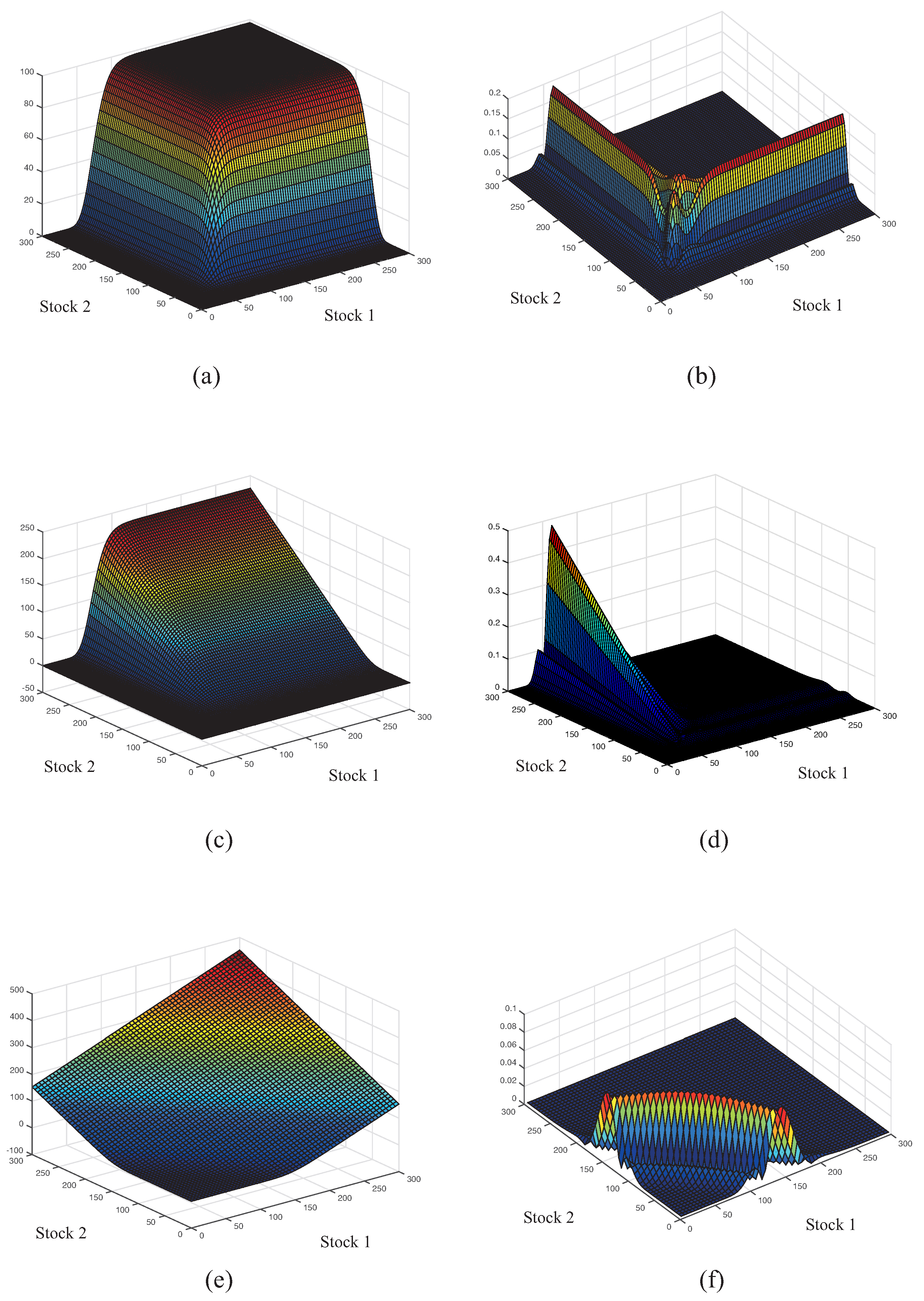
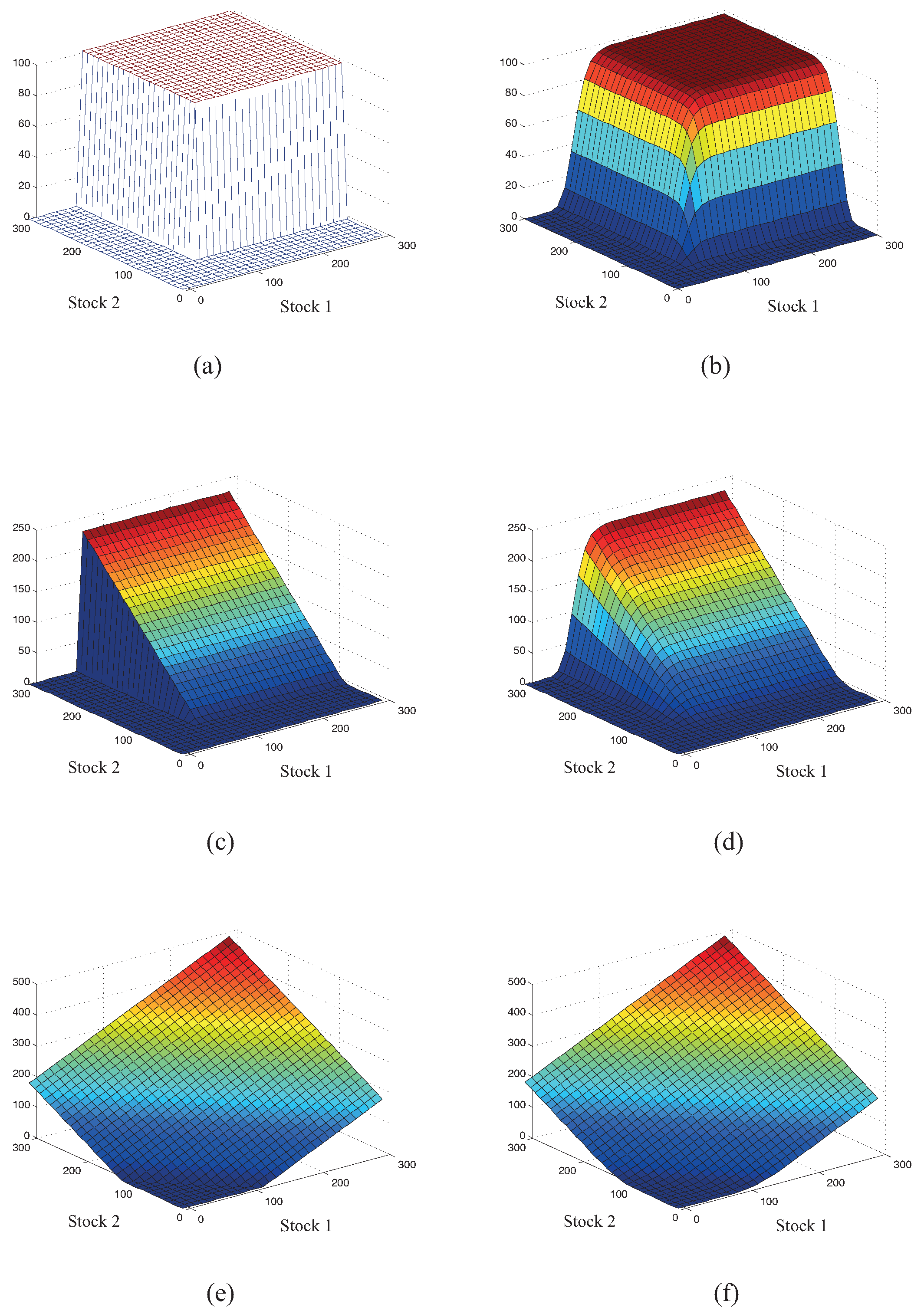
- (1)
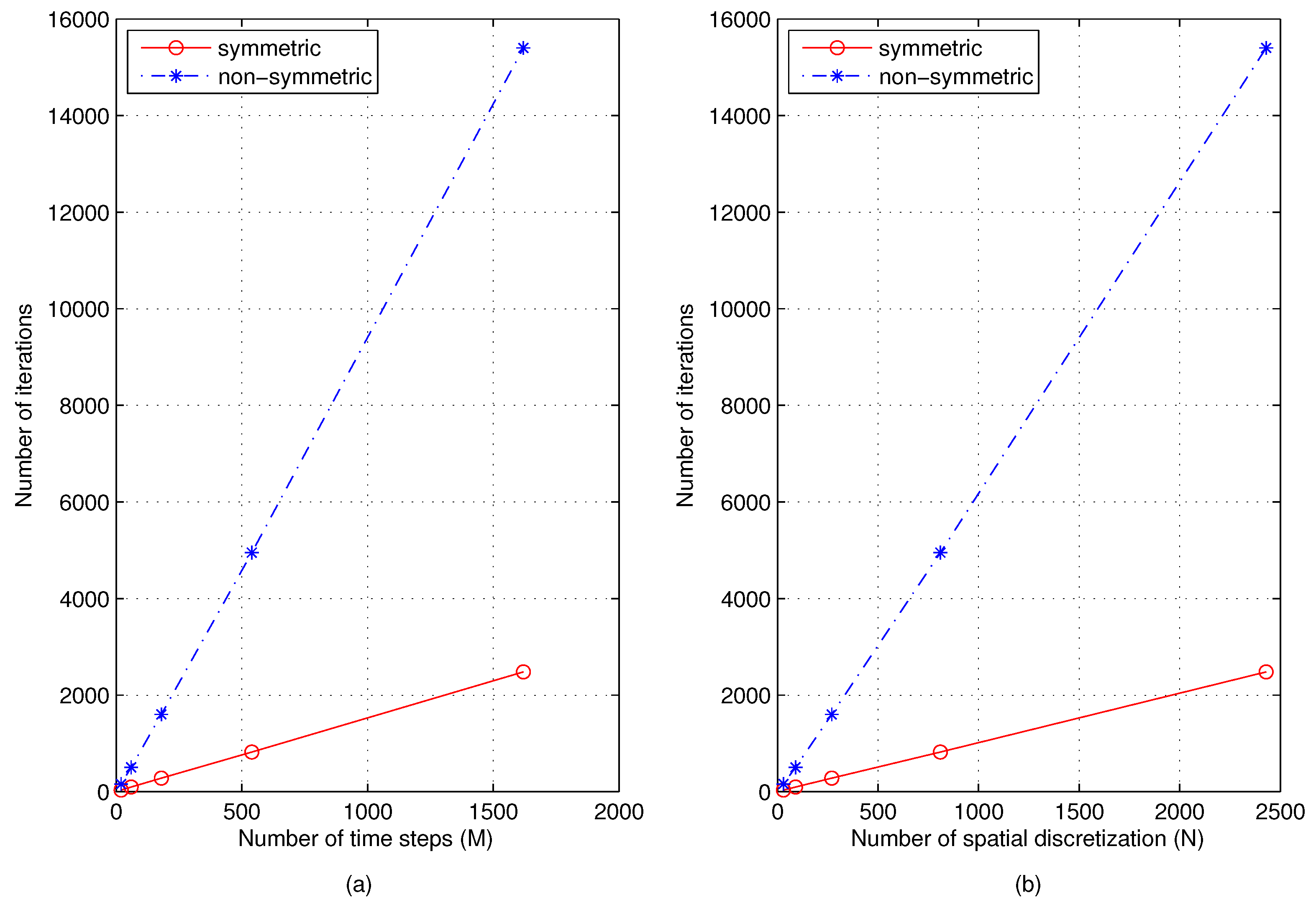
- Cash or Nothingwith parameters: Figure 1a,b shows and , respectively.
- (2)
- (3)
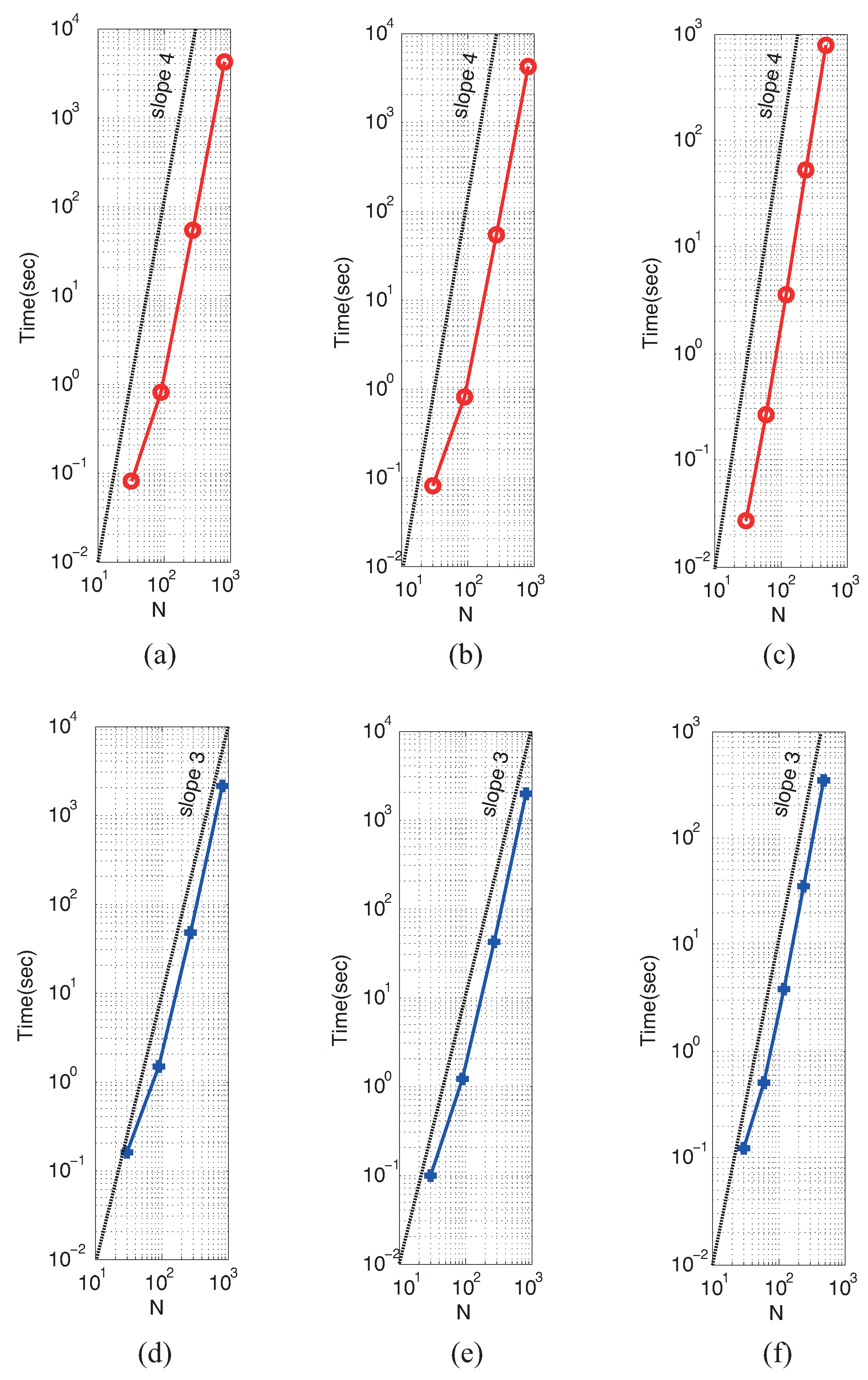
5.2. Computational Cost
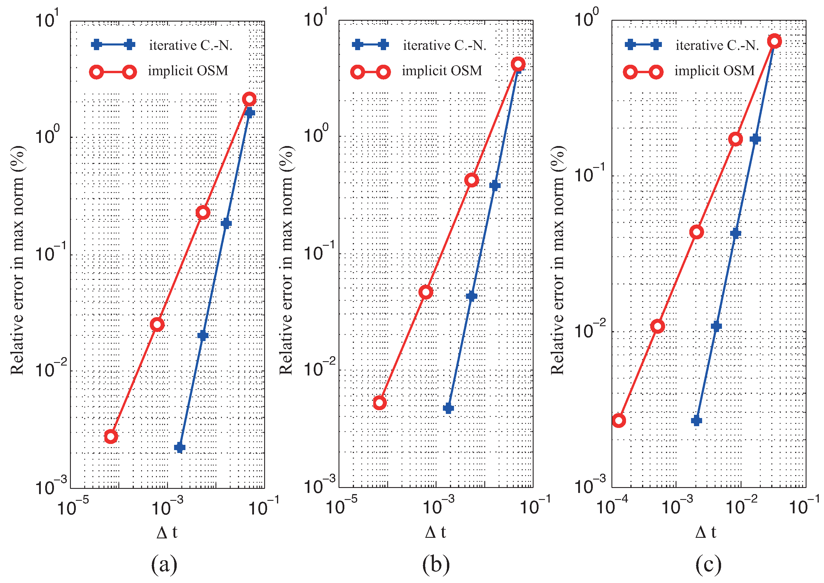
5.3. Order of Convergence in Space and Time
6. Conclusions
Acknowledgments
Author Contributions
Conflicts of Interest
References
- Daoud, Y.; Özis, T. The Operator Splitting Method for Black–Scholes Equation. Appl. Math. 2011, 2, 771–778. [Google Scholar] [CrossRef]
- Duffy, D.J. Finite Difference Methods in Financial Engineering: A Partial Differential Approach; John Wiley and Sons: New York, NY, USA, 2006. [Google Scholar]
- Jeong, D.; Kim, J. A comparison study of ADI and operator splitting methods on option pricing models. J. Comput. Appl. Math. 2013, 247, 162–171. [Google Scholar] [CrossRef]
- Cavoretto, R. A numerical algorithm for multidimensional modeling of scattered data points. Comput. Appl. Math. 2015, 34, 65–80. [Google Scholar] [CrossRef]
- Shcherbakov, V.; Larsson, E. Radial basis function partition of unity methods for pricing vanilla basket options. Comput. Math. Appl. 2016, 71, 185–200. [Google Scholar] [CrossRef]
- Oosterlee, C.W.; Leentvaar, C.C.; Huang, X. Accurate American Option Pricing by Grid Stretching and High Order Finite Differences; Technical Report; Delft University of Technology: Delft, The Netherlands, 2005. [Google Scholar]
- Le Floc’h, F. TR-BDF2 for Stable American Option Pricing. J. Comput. Finance 2014, 17, 31–56. [Google Scholar] [CrossRef]
- Hull, J.C. Options, Futures and Other Derivatives, 9 ed.; Prentice Hall: Upper Saddle River, NJ, USA, 2014. [Google Scholar]
- Wilmott, P. Paul Wilmott on Quantitative Finance, 2 ed.; Wiley: Hoboken, NJ, USA, 2006. [Google Scholar]
- Zhu, Y.L.; Wu, X.; Chern, I. Derivative Securities and Difference Methods; Springer: Berlin, Germany, 2004. [Google Scholar]
- Morton, K.W.; Mayers, D. Numerical Solution of Partial Differential Equations, 2 ed.; Cambridge University Press: Cambridge, UK, 2005. [Google Scholar]
- Saad, Y. Iterative Methods for Sparse Linear Systems, 2 ed.; SIAM: Philadelphia, PA, USA, 2003. [Google Scholar]
- Saad, Y.; Schultz, M.H. GMRES: A generalized minimal residual algorithm for solving nonsymmetric linear systems. SIAM J. Sci. Stat. Comput. 1986, 7, 856–869. [Google Scholar] [CrossRef]
- Mittal, R.; Al-Kurdi, A. An efficient method for constructing an ILU preconditioner for solving large sparse nonsymmetric linear systems by the GMRES method. Comput. Math. Appl. 2003, 45, 1757–1772. [Google Scholar] [CrossRef]
- Trefethen, L.N.; Iii, D.B. Numerical Linear Algebra; SIAM: Philadelphia, PA, USA, 1997. [Google Scholar]
- Krekel, M.; de Kock, J.; Korn, R.; Man, T.K. An Analysis of Pricing Methods for Baskets Options; Wilmott: Soissons, France, 2004; pp. 82–89. [Google Scholar]
- Haug, E.G. The Complete Guide to Option Pricing Formulas; McGraw-Hill Education: New York, NY, USA, 2006. [Google Scholar]
- Ju, N. Pricing Asian and Basket options via taylor expansion. J. Comput. Financ. 2002, 5, 79–103. [Google Scholar] [CrossRef]
- Han, C. Finite Difference Method with GMRES Solver for the 2D Black–Scholes Equation. Master’s Thesis, Korea University, Seoul, Korea, 2014. [Google Scholar]


| Option Type | Numerical Method | Rel. Err (%) | Ratio | Time (s) | ||
|---|---|---|---|---|---|---|
| (1) Cash or Nothing | ||||||
| Iterative-Crank–Nicolson | 1/30 | 1/20 | 3.5 | - | 0.1 | |
| 1/90 | 1/60 | 0.34 | 10 | 1.5 | ||
| 1/270 | 1/180 | 0.037 | 9.2 | 47 | ||
| 1/810 | 1/540 | 0.0044 | 8.3 | 2000 | ||
| OSM | 1/30 | 1/20 | 4.0 | - | 0.08 | |
| 1/90 | 1/180 | 0.39 | 10 | 0.8 | ||
| 1/270 | 1/1620 | 0.042 | 9.3 | 5.4 | ||
| 1/810 | 1/14580 | 0.0046 | 9.0 | 4200 | ||
| (2) Call | ||||||
| Iterative-Crank–Nicolson | 1/30 | 1/20 | 1.6 | - | 0.1 | |
| 1/90 | 1/60 | 0.21 | 7.6 | 1.2 | ||
| 1/270 | 1/180 | 0.024 | 8.8 | 43 | ||
| 1/810 | 1/540 | 0.0026 | 9.4 | 1900 | ||
| OSM | 1/30 | 1/20 | 1.9 | - | 0.03 | |
| 1/90 | 1/180 | 0.25 | 7.4 | 0.8 | ||
| 1/270 | 1/1620 | 0.028 | 9.2 | 54 | ||
| 1/810 | 1/14580 | 0.0030 | 9.0 | 4300 | ||
| (3) Basket | ||||||
| Iterative-Crank–Nicolson | 1/30 | 1/30 | 0.71 | - | 0.1 | |
| 1/60 | 1/60 | 0.17 | 4.2 | 0.5 | ||
| 1/120 | 1/120 | 0.042 | 4.0 | 4 | ||
| 1/240 | 1/240 | 0.011 | 4.0 | 35 | ||
| 1/480 | 1/480 | 0.0026 | 4.0 | 340 | ||
| OSM | 1/30 | 1/30 | 0.73 | - | 0.03 | |
| 1/60 | 1/120 | 0.17 | 4.2 | 0.3 | ||
| 1/120 | 1/480 | 0.043 | 4.0 | 3.6 | ||
| 1/240 | 1/1920 | 0.011 | 4.0 | 6 | ||
| 1/480 | 1/7680 | 0.0026 | 4.0 | 780 |
| Option Type | Numerical Method | Rel. Err. (%) | Memory (Mb) | Time (s) | ||
|---|---|---|---|---|---|---|
| (1) Cash or Nothing | ||||||
| Iterative-Crank–Nicolson | 1/30 | 1/20 | 1.68 | 18 | 0.8 | |
| 1/90 | 1/60 | 0.19 | 345 | 15 | ||
| 1/270 | 1/180 | 0.02 | 8430 | 346 | ||
| OSM | 1/30 | 1/20 | 2.15 | 5 | 1.3 | |
| 1/90 | 1/60 | 0.37 | 30 | 30 | ||
| 1/270 | 1/180 | 0.09 | 252 | 771 | ||
| (2) Call | ||||||
| Iterative-Crank–Nicolson | 1/30 | 1/20 | 1.6 | 18 | 0.8 | |
| 1/90 | 1/60 | 0.21 | 345 | 13 | ||
| 1/270 | 1/180 | 0.02 | 8477 | 283 | ||
| OSM | 1/30 | 1/20 | 1.9 | 4 | 1.2 | |
| 1/90 | 1/60 | 0.33 | 15 | 29 | ||
| 1/270 | 1/180 | 0.06 | 159 | 756 | ||
| (3) Basket | ||||||
| Iterative-Crank–Nicolson | 1/30 | 1/30 | 0.47 | 1.8 | 0.9 | |
| 1/60 | 1/60 | 0.12 | 24 | 5.8 | ||
| 1/120 | 1/120 | 0.03 | 993 | 33 | ||
| OSM | 1/30 | 1/30 | 0.49 | 2 | 1.6 | |
| 1/60 | 1/60 | 0.12 | 8.6 | 12 | ||
| 1/120 | 1/120 | 0.04 | 45 | 96.9 |
© 2017 by the authors; licensee MDPI, Basel, Switzerland. This article is an open access article distributed under the terms and conditions of the Creative Commons Attribution (CC BY) license (http://creativecommons.org/licenses/by/4.0/).
Share and Cite
Pak, D.; Han, C.; Hong, W.-T. Iterative Speedup by Utilizing Symmetric Data in Pricing Options with Two Risky Assets. Symmetry 2017, 9, 12. https://doi.org/10.3390/sym9010012
Pak D, Han C, Hong W-T. Iterative Speedup by Utilizing Symmetric Data in Pricing Options with Two Risky Assets. Symmetry. 2017; 9(1):12. https://doi.org/10.3390/sym9010012
Chicago/Turabian StylePak, Dohyun, Changkyu Han, and Won-Tak Hong. 2017. "Iterative Speedup by Utilizing Symmetric Data in Pricing Options with Two Risky Assets" Symmetry 9, no. 1: 12. https://doi.org/10.3390/sym9010012