Non-Local Meta-Conformal Invariance, Diffusion-Limited Erosion and the XXZ Chain

Abstract

Diffusion-limited erosion is a distinct universality class of fluctuating interfaces. Although its dynamical exponent $z=1$, none of the known variants of conformal invariance can act as its dynamical symmetry. In $d=1$ spatial dimensions, its infinite-dimensional dynamic symmetry is constructed and shown to be isomorphic to the direct sum of three loop-Virasoro algebras. The infinitesimal generators are spatially non-local and use the Riesz-Feller fractional derivative. Co-variant two-time response functions are derived and reproduce the exact solution of diffusion-limited erosion. The relationship with the terrace-step-kind model of vicinal surfaces and the integrable XXZ chain are discussed.

1. Introduction

Symmetries have since a long time played an important role in the analysis of physical systems. The insight gained can be either calculational, in that a recognised symmetry becomes useful in simplifying calculations, or else conceptual, in that the identification of symmetries can lead to new level of understanding. In the statistical physics of equilibrium second-order phase transitions in two dimensions, conformal invariance has ever since the pioneering work of Belavin, Polyakov and Zamolodchikov [1] created considerable progress, both computationally as well as conceptually. It then appears natural to ask if one might find extensions of conformal invariance which apply to time-dependent phenomena. Here, we shall inquire about dynamical symmetries of the following stochastic Langevin equation, to be called diffusion-limited erosion (dle) Langevin equation, which reads in momentum space [2]

$$\mathrm{d}\widehat{h}(t,\mathit{q})=-\nu |\mathit{q}|\widehat{h}(t,\mathit{q})\mathrm{d}t+\widehat{j}(t,\mathit{q})\mathrm{d}t+{\left(2\nu T\right)}^{1/2}\mathrm{d}\widehat{B}(t,\mathit{q})$$

(1)

and describes the Fourier-transformed height $\widehat{h}(t,\mathit{q})={(2\pi )}^{-d/2}{\int }_{{\mathbb{R}}^d}\mathrm{d}\mathit{r}{e}^{-\mathrm{i}\mathit{q}·\mathit{r}}h(t,\mathit{r})$. Because of the (Fourier-transformed) standard brownian motion $\widehat{B}$, with the variance $\langle \widehat{B}(t,\mathit{q})\widehat{B}(t^{\prime },{\mathit{q}}^{\prime })\rangle =min(t,t^{\prime })\delta (\mathit{q}+{\mathit{q}}^{\prime })$, this is a stochastic process, called diffusion-limited erosion (dle) process. Herein, $\nu ,T$ are non-negative constants and $\delta (\mathit{q})$ is the Dirac distribution. Since we shall be interested in deriving linear responses, an external infinitesimal source term $\widehat{j}(t,\mathit{q})$ is also included, to be set to zero at the end. Inverting the Fourier transform in order to return to direct space, Equation (1) implies spatially long-range interactions. The conformal invariance of equilibrium critical systems with long-range interactions has been analysed recently [3]. Equation (1) arises in several distinct physical contexts.

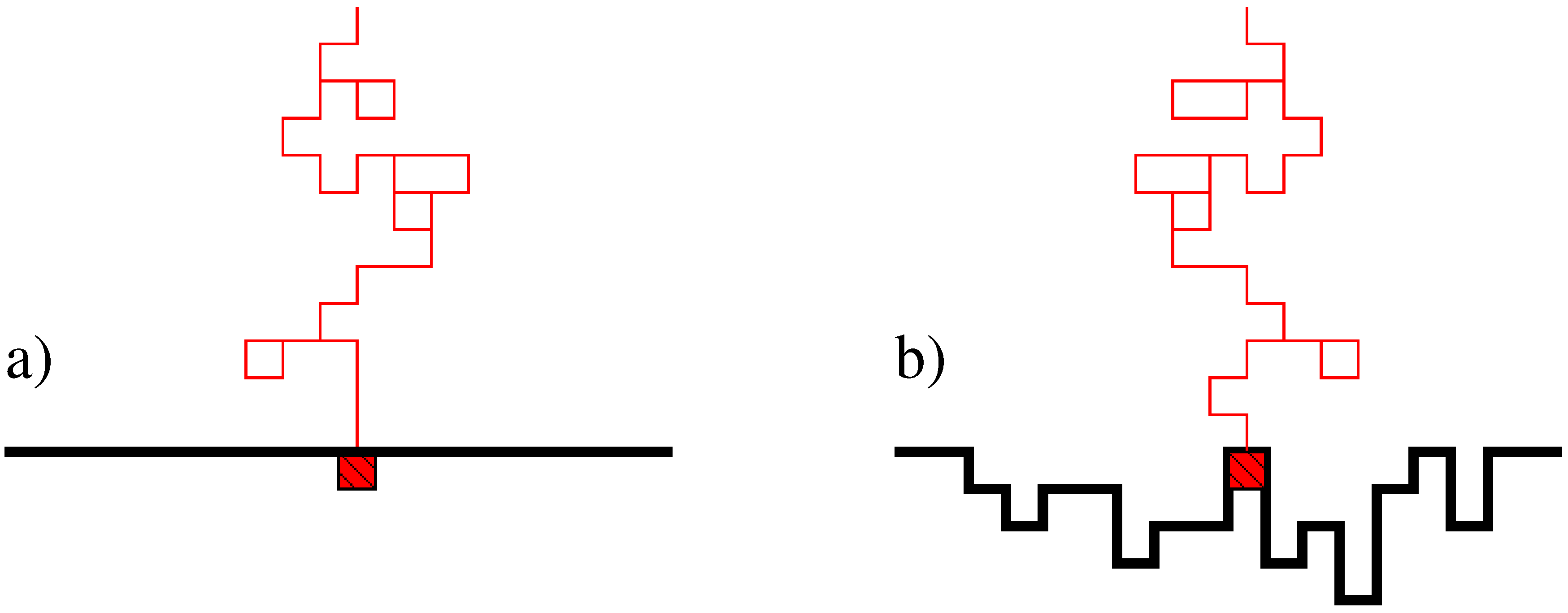
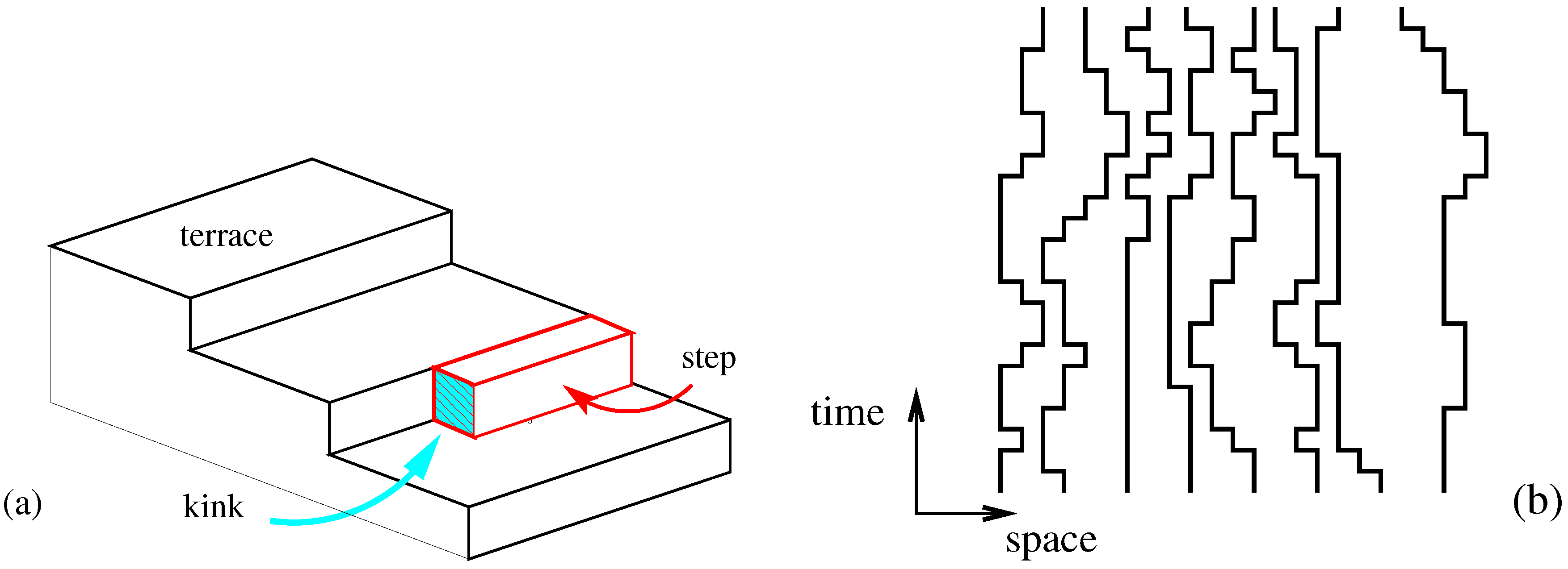
Example 1.

For the original definition of the (dle) process [2], one considers how an initially flat interface is affected by the diffusive motion of corrosive particles. A single corrosive particle starts initially far away from the interface. After having undergone diffusive motion until the particle finally arrives at the interface, it erodes a particle from that interface. Repeating this process many times, an eroding interface forms which is described in terms of a fluctuating height $h(t,\mathit{r})$, see Figure 1. It can be shown that this leads to the dle Langevin Equation (1) [2,4].

Several lattice formulations of the model [2,5,6,7] confirm the dynamical exponent $z=1$.

Example 2.

A different physical realisation of Equation (1) invokes vicinal surfaces. Remarkably, for $d=1$ space dimension, the Langevin Equation (1) has been argued [8] to be related to a system of non-interacting fermions, conditioned to an a-typically large flux. Consider the terrace-step-kink model of a vicinal surface, and interpret the steps as the world lines of fermions, see Figure 2. Its transfer matrix is the matrix exponential of the quantum hamiltonian H of the asymmetric XXZ chain [8]. Use Pauli matrices ${\sigma }_n^{\pm ,z}$, attached to each site n, such that the particle number at each site is ${\varrho }_n=\frac{1}{2}\left(1+{\sigma }_n^z\right)=0,1$. On a chain of N sites, consider the quantum hamiltonian [8,9,10]

$$H=-\frac{w}{2}\sum _{n=1}^N\left[2v{\sigma }_n^{+}{\sigma }_{n+1}^{-}+2v^{-1}{\sigma }_n^{-}{\sigma }_{n+1}^{+}+\mathrm{\Delta }\left({\sigma }_n^z{\sigma }_{n+1}^z-1\right)\right]$$

(2)

where $w=\sqrt{pq}{e}^{\mu }$, $v=\sqrt{p/q}{e}^{\lambda }$ and $\mathrm{\Delta }=2\left(\sqrt{p/q}+\sqrt{q/p}\right)e^{-\mu }$. Herein, $p,q$ describe the left/right bias of single-particle hopping and $\lambda ,\mu$ are the grand-canonical parameters conjugate to the current and the mean particle number. In the continuum limit, the particle density ${\varrho }_n(t)\to \varrho (t,r)={\partial }_{r}h(t,r)$ is related to the height h which in turn obeys (1), with a gaussian white noise η [8]. This follows from the application of the theory of fluctuating hydrodynamics, see [11,12] for recent reviews. The low-energy behaviour of H yields the dynamical exponent $z=1$ [8,9,10]. If one conditions the system to an a-typically large current, the large-time, large-distance behaviour of (2) has very recently been shown [10] (i) to be described by a conformal field-theory with central charge $c=1$ and (ii) the time-space scaling behaviour of the stationary structure function has been worked out explicitly, for $\lambda \to \infty$. Therefore, one may conjecture that the so simple-looking Equation (1) should furnish an effective continuum description of the large-time, long-range properties of quite non-trivial systems, such as (2).

The physical realisation of Equation (1) in terms of the dle process makes it convenient to discuss the results in terms of the physics of the growth of interfaces [13,14,15], which can be viewed as a paradigmatic example of the emergence of non-equilibrium collective phenomena [16,17]. Such an interface can be described in terms of a time-space-dependent height profile $h(t,\mathit{r})$. This profile depends also on the eventual fluctuations of the set of initial states and on the noise in the Langevin equation, hence h should be considered as a random variable. The degree of fluctuations can be measured through the interface width. If the model is formulated first on a hyper-cubic lattice $\mathcal{L}\subset {\mathbb{Z}}^d$ of $|\mathcal{L}|=L^d$ sites, the interface width is defined by

$$w^2(t;L):=\frac{1}{L^d}\sum _{\mathit{r}\in \mathcal{L}}{〈\left(h(t,\mathit{r})-\overline{h}(t)\right)〉}^2=L^{2\beta z}{f}_w\left(t{L}^{-z}\right)\sim \left\{\begin{array}{cc}{t}^{2\beta }\hfill & ;\mathrm{if}{tL}^{-\mathrm{z}}\ll 1\hfill \\ L^{2\beta z}\hfill & ;\mathrm{if}{tL}^{-\mathrm{z}}\gg 1\hfill \end{array}\right.$$

(3)

where the generically expected scaling form, for large times/lattice sizes $t\to \infty$, $L\to \infty$, is also indicated. Physicists call this Family-Vicsek scaling [18]. Implicitly, it is assumed here that one is not at the ‘upper critical dimension $d^{*}$’, where this power-law scaling is replaced by a logarithmic scaling form, see also below. Herein, $\langle .\rangle$ denotes an average over many independent samples and $\overline{h}(t):=L^{-d}{\sum }_{\mathit{r}\in \mathcal{L}}h(t,\mathit{r})$ is the spatially averaged height. Furthermore, β is called the growth exponent, $z>0$ is the dynamical exponent and $\alpha :=\beta z$ is the roughness exponent. When $t{L}^{-z}\gg 1$, one speaks of the saturation regime and when $t{L}^{-z}\ll 1$, one speaks of the growth regime. We shall focus on the growth regime from now on.

Definition 1.

On a spatially infinite substrate, an interface with a width $w(t)\nearrow \infty$ for large times $t\to \infty$ is called rough. If ${lim}_{t\to \infty }w(t)$ is finite, the interface is called smooth.

This definition permits a first appreciation of the nature of the interface: if in (3) $\beta >0$, the interface is rough.

In addition, dynamical properties of the interface can be studied through the two-time correlators and responses. In the growth regime (where effectively $L\to \infty$), one considers the double scaling limit $t,s\to \infty$ with $y:=t/s>1$ fixed and expects the scaling behaviour

$$\begin{array}{cc}\hfill C(t,s;\mathit{r})& :=〈\left(h(t,\mathit{r})-〈\overline{h}(t)〉\right)\left(h(s,\mathbf{0})-〈\overline{h}(s)〉\right)〉=s^{-b}{F}_C\left(\frac{t}{s};\frac{\mathit{r}}{s^{1/z}}\right)\hfill \end{array}$$

(4a)

$$\begin{array}{cc}\hfill R(t,s;\mathit{r})& :={\left.\frac{\delta 〈h(t,\mathit{r})-\overline{h}(t)〉}{\delta j(s,\mathbf{0})}\right|}_{j=0}=〈h(t,\mathit{r})\tilde{h}(s,\mathbf{0})〉=s^{-1-a}{F}_R\left(\frac{t}{s};\frac{\mathit{r}}{s^{1/z}}\right)\hfill \end{array}$$

(4b)

where j is an external field conjugate to the height h. Throughout, all correlators are calculated with $j=0$. In the context of Janssen-de Dominicis theory, $\tilde{h}$ is the conjugate response field to h, see [17]. Spatial translation-invariance was implicitly admitted in (4). This defines the ageing exponents $a,b$. The autocorrelation exponent ${\lambda }_C$ and the autoresponse exponent ${\lambda }_R$ are defined from the asymptotics $F_{C,R}(y,\mathbf{0})\sim y^{-{\lambda }_{C,R}/z}$ as $y\to \infty$. For these non-equilibrium exponents, one has $b=-2\beta$ [15] and the bound ${\lambda }_C\ge (d+zb)/2$ [19,20].

For the dle process, these exponents are readily found form the exact solution of (1) [2,4,21]. For an initially flat interface $h(0,\mathit{r})=0$, the two-time correlator and response are in Fourier space

$$\begin{array}{cc}\hfill \widehat{C}(t,s;\mathit{q},{\mathit{q}}^{\prime })& :=〈\widehat{h}(t,\mathit{q})\widehat{h}(s,{\mathit{q}}^{\prime })〉=\frac{T}{|\mathit{q}|}\left[e^{-\nu |\mathit{q}||t-s|}-e^{-\nu |\mathit{q}|(t+s)}\right]\delta (\mathit{q}+{\mathit{q}}^{\prime }),\hfill \end{array}$$

(5a)

$$\begin{array}{cc}\hfill \widehat{R}(t,s;\mathit{q},{\mathit{q}}^{\prime })& :={\left.\frac{\delta \langle \widehat{h}(t,\mathit{q})\rangle }{\delta \widehat{j}(s,{\mathit{q}}^{\prime })}\right|}_{j=0}=\mathrm{\Theta }(t-s)e^{-\nu |\mathit{q}|(t-s)}\delta (\mathit{q}+{\mathit{q}}^{\prime }).\hfill \end{array}$$

(5b)

In direct space, this becomes, for $d\ne 1$ and with ${\mathcal{C}}_0:=\mathrm{\Gamma }((d+1)/2)/(\mathrm{\Gamma }(d/2){\pi }^{(d+1)/2})$

$$\begin{array}{cc}\hfill C(t,s;\mathit{r})& =\frac{T{\mathcal{C}}_0}{d-1}\left[{\left({\nu }^2{(t-s)}^2+r^2\right)}^{-(d-1)/2}-{\left({\nu }^2{(t+s)}^2+r^2\right)}^{-(d-1)/2}\right]\hfill \end{array}$$

(6a)

$$\begin{array}{cc}\hfill R(t,s;\mathit{r})& ={\mathcal{C}}_0\mathrm{\Theta }(t-s)\nu (t-s){\left({\nu }^2{(t-s)}^2+r^2\right)}^{-(d+1)/2}\hfill \end{array}$$

(6b)

where the Heaviside function Θ expresses the causality condition $t>s$. In particular, in the growth regime, the interface width reads (where ${\mathcal{C}}_1(\mathrm{\Lambda })$ is a known constant and a high-momentum cut-off Λ was used for $d>1$)

$$w^2(t)=C(t,t;\mathbf{0})=\frac{T{\mathcal{C}}_0}{1-d}\left[{\left(2\nu t\right)}^{1-d}-{\mathcal{C}}_1(\mathrm{\Lambda })\right]\stackrel{t\to \infty }{\simeq }\left\{\begin{array}{cc}T{\mathcal{C}}_0{\mathcal{C}}_1(\mathrm{\Lambda })/(d-1)\hfill & ;\mathrm{if}d>1\hfill \\ T{\mathcal{C}}_{0}ln(2\nu t)\hfill & ;\mathrm{if}d=1\hfill \\ T{\mathcal{C}}_0{(2\nu )}^{1-d}/(1-d)·t^{1-d}\hfill & ;\mathrm{if}d<1\hfill \end{array}\right.$$

(7)

Hence $d^{*}=1$ is the upper critical dimension of the dle process. It follows that at late times the dle-interface is smooth for $d>1$ and rough for $d\le 1$. On the other hand, one may consider the stationary limit $t,s\to \infty$ with the time difference $\tau =t-s$ being kept fixed. Then one finds a fluctuation-dissipation relation $\partial C(s+\tau ,s;\mathit{r})/\partial \tau =-\nu TR(s+\tau ,s;\mathit{r})$. The similarity of this to what is found for equilibrium systems is unsurprising, since several discrete lattice variants of the dle process exist and are formulated as an equilibrium system [5]. Lastly, the exponents defined above are read off by taking the scaling limit, and are listed in

Table 1. Exponents of growing interfaces in the Kardar-Parisi-Zhang (kpz), Edwards-Wilkinson (ew), Arcetri (for both $T=T_c$ and $T<T_c$) and dle universality classes. The numbers in bracket give the estimated error in the last digit(s).

Model	d	z	β	a	b	${\mathit{\lambda }}_{\mathit{C}}$	${\mathit{\lambda }}_{\mathit{R}}$	References
kpz	1	$3/2$	$1/3$	$-1/3$	$-2/3$	1	1	[25,29,32]
	2	$1.61(2)$	$0.2415(15)$	$0.30(1)$	$-0.483(3)$	$1.97(3)$	$2.04(3)$	[33,34]
	2	$1.61(2)$	$0.241(1)$	-	$-0.483$	$1.91(6)$	-	[35]
	2	$1.61(5)$	$0.244(2)$	-	-	-	-	[26]
	2	$1.627(4)$	$0.229(6)$	-	-	-	-	[36]
	2	$1.61(2)$	$0.2415(15)$	$0.24(2)$	$-0.483(3)$	$1.97(3)$	$2.00(6)$	[31,33]
ew	$<2$	2	$(2-d)/4$	$d/2-1$	$d/2-1$	d	d
	2	2	0(log)${}^{\#}$	0	0	2	2	[24,37]
	$>2$	2	0	$d/2-1$	$d/2-1$	d	d
Arcetri $T=T_c$	$<2$	2	$(2-d)/4$	$d/2-1$	$d/2-1$	$3d/2-1$	$3d/2-1$
	2	2	0(log)${}^{\#}$	0	0	2	2	[20]
	$>2$	2	0	$d/2-1$	$d/2-1$	d	d
$T<T_c$	d	2	$1/2$	$d/2-1$	$-1$	$d/2-1$	$d/2-1$
dle	$<1$	1	$(1-d)/2$	$d-1$	$d-1$	d	d
	1	1	0(log)${}^{\#}$	0	0	1	1	[4,21]
	$>1$	1	0	$d-1$	$d-1$	d	d

${}^{\#}$ For $d=d^{*}$, one has logarithmic scaling $w{(t;L)}^2\sim lnt{f}_w\left(lnL/lnt\right)$.

. In contrast to the interface width $w(t)$, which shows a logarithmic growth at $d=d^{*}=1$, logarithms cancel in the two-time correlator C and response R, up to additive logarithmic corrections to scaling. This is well-known in the physical ageing at $d=d^{*}$ of simple magnets [22,23] or of the Arcetri model [20].

For comparison, we also list in Table 1 values of the non-equilibrium exponents for several other universality classes of interface growth. In particular, one sees that for the Edwards-Wilkinson (ew) [24] and Arcetri classes, the upper critical dimension $d^{*}=2$, while it is still unknown if a finite value of $d^{*}$ exists for the Kardar-Parisi-Zhang (kpz) class, see [13,14,25,26,27,28]. Clearly, the stationary exponents $a,b,z$ are the same in the ew and Arcetri classes, but the non-equilibrium relaxation exponents ${\lambda }_C,{\lambda }_R$ are different for dimensions $d<d^{*}$. This illustrates the independence of ${\lambda }_C,{\lambda }_R$ from those stationary exponents, in agreement with studies in the non-equilibrium critical dynamics of relaxing magnetic systems. On the other hand, for the kpz class, a perturbative renormalisation-group analysis shows that ${\lambda }_C=d$ for $d<2$ [29]. For $d>2$, a new strong-coupling fixed point arises and the relaxational properties are still unknown. Even for $d=2$, the results of different numerical studies in the kpz class are not yet fully consistent, but recent simulations suggest that precise information on the shape of the scaling function, coming from a dynamical symmetry [30], may improve the quality of the extracted exponents [31].

Here, we are concerned with the dynamical symmetries of the dle process. Our main results are as follows.

Theorem 1.

The dynamical symmetry of the dle process, in $d=1$ space dimension and with $j=0$, is a meta-conformal algebra, in a sense to be made more precise below, and is isomorphic to the direct sum of three Virasoro algebras without central charge (or loop-Virasoro algebra). The Lie algebra generators will be given below in Equation (29), they are non-local in space. The general form of the co-variant two-time response function is (with $t>s$)

$$\begin{array}{c}{\displaystyle R(t,s;r)=F_A{(t-s)}^{1-2x}\frac{\nu (t-s)}{{\nu }^2{(t-s)}^2+r^2}}\hfill \\ +F_B{(t-s)}^{1+\psi -2x}{\left({\nu }^2{(t-s)}^2+r^2\right)}^{-(\psi +1)/2}cos\left((\psi +1)arctan\left(\frac{r}{\nu (t-s)}\right)-\frac{\pi \psi }{2}\right)\hfill \end{array}$$

(8)

where $x,\psi$ are real parameters and $F_{A,B}$ are normalisation constants.

Remark 1.

The exact solution (6b) of the dle-response in $(1+1)D$ is reproduced by (8) if one takes $x=\frac{1}{2}$, $\nu >0$, $F_A={\mathcal{C}}_0$ and $F_B=0$. This illustrates the importance of non-local generators in a specific physical application.

Remark 2.

The symmetries so constructed are only dynamical symmetries of the so-called ‘deterministic part’ of Equation (1), which is obtained by setting $T=0$. We shall see that the co-variant two-time correlator $C(t,s;r)=0$. This agrees with the vanishing of the exact dle-correlator (6a) in the $T\to 0$ limit (fix $d\ne 1$ and let first $T\to 0$ and only afterwards $d\to 1$).

This paper presents an exploration of the dynamical symmetries of dle process for $d=1$ and is organised as follows. In Section 2, we introduce the distinction of ortho-conformal and meta-conformal invariance and illustrate these notions by several examples, see

Table 2. Comparison of local ortho-conformal, conformal Galilean and meta-1 conformal invariance, in $(1+1)D$. The non-vanishing Lie algebra commutators, the defining equation of the generators, the invariant differential operator $\mathcal{S}$ and the covariant two-point function is indicated, where applicable. Physically, the co-variant quasiprimary two-point function ${\mathcal{C}}_{12}=\langle {\phi }_1(t,r){\phi }_2(0,0)\rangle$ is a correlator, with the constraints $x_1=x_2$ and ${\gamma }_1={\gamma }_2$.

	Ortho	Galilean	Meta-1
Lie	$\left[X_n,X_m\right]=(n-m)X_{n+m}$	$\left[X_n,X_m\right]=(n-m)X_{n+m}$	$\left[X_n,X_m\right]=(n-m)X_{n+m}$
algebra	$\left[X_n,Y_m\right]=(n-m)Y_{n+m}$	$\left[X_n,Y_m\right]=(n-m)Y_{n+m}$	$\left[X_n,Y_m\right]=(n-m)Y_{n+m}$
	$\left[Y_n,Y_m\right]=(n-m)X_{n+m}$	$\left[Y_n,Y_m\right]=0$	$\left[Y_n,Y_m\right]=\mu (n-m)Y_{n+m}$
generators	(9)	(15)	(13)
$\mathcal{S}$	${\partial }_t^2+{\partial }_r^2$	-	$-\mu {\partial }_t+{\partial }_r$
${\mathcal{C}}_{12}$	$t^{-2x_1}{\left(1+{\left(\frac{r}{t}\right)}^2\right)}^{-x_1}$	$t^{-2x_1}exp\left(-2\left|\frac{{\gamma }_{1}r}{t}\right|\right)$	$t^{-2x_1}{\left(1+\frac{\mu }{{\gamma }_1}\left|\frac{{\gamma }_{1}r}{t}\right|\right)}^{-2{\gamma }_1/\mu }$

. In Section 3, we explain why none of these local symmetries can be considered as a valid candidate of the dynamical symmetry of the dle process. Section 4 presents some basic properties on the Riesz-Feller fractional derivative which are used in Section 5 to explicitly construct the non-local dynamical symmetry of the dle process, thereby generalising and extending earlier results [21]. Section 6 outlines the formulation of time-space Ward identities for the computation of covariant n-point functions and in Section 7 the two-point correlator and response are found for the dynamical symmetry of the dle process. The propositions proven in Section 5 and Section 7 make the Theorem 1 more precise and constitute its proof. The Lie algebra contraction, in the limit $\nu \to \infty$, and its relationship with the conformal Galilean algebra is briefly mentioned. This is summarised in

Table 3. Comparison of non-local meta-2 conformal invariance, and meta-conformal galilei invariance in $(1+1)D$. The non-vanishing Lie algebra commutators, the defining equation of the generators and the invariant differential operator $\mathcal{S}$ are indicated. The usual generators are $X_n=A_n+B_n^{+}+B_n^{-}$, $Y_n=B_n^{+}+B_n^{-}$ and $Z_n=B_n^{+}-B_n^{-}$, see also Table 2. Physically, the co-variant quasiprimary two-point function ${\mathcal{R}}_{12}=\langle {\phi }_1(t,r){\tilde{\phi }}_2(0,0)\rangle$ is a response function. In case B, one has $\psi =2{\xi }_1-1$.

	Meta-2 Conformal	Meta-Conformal Galilean	Constraints
Lie	$\left[A_n,A_m\right]=(n-m)A_{n+m}$	$\left[X_n,X_m\right]=(n-m)X_{n+m}$
algebra	$\left[B_n^{\pm },B_m^{\pm }\right]=(n-m)B_{n+m}^{\pm }$	$\left[X_n,B_m^{\pm }\right]=(n-m)B_{n+m}^{\pm }$
generators	(29)	(43)
$\mathcal{S}$	$-\mu {\partial }_t+{\mathrm{\nabla }}_r$	-
${\mathcal{R}}_{12}$	$t^{1-x_1-x_2}·\nu t{\left({\nu }^2{t}^2+r^2\right)}^{-1}$	-	${\xi }_1+{\xi }_2=1$   (A) $x_1-{\xi }_1=x_2-{\xi }_2$
	$t^{2{\xi }_1-2x_1}{\left({\nu }^2{t}^2+r^2\right)}^{-{\xi }_1}$ $·sin\left[\pi {\xi }_1-2{\xi }_{1}arctan\left(\frac{r}{\nu t}\right)\right]$	$t^{-2x_1}exp\left(-2\left|{\gamma }_{1}r/t\right|\right)$	$x_1=x_2$   (B) ${\xi }_1={\xi }_2$, or ${\gamma }_1={\gamma }_2$

.

2. Local Conformal Invariance

Can one explain the form of the two-time scaling functions of the dle process in terms of a dynamical symmetry? To answer such a question, one must first formulate it more precisely.

Definition 2.

The deterministic part of the Langevin Equation (1) is obtained when formally setting $\widehat{B}=0$.

Our inspiration comes from Niederer’s treatment [38] of the dynamical symmetries of the free diffusion equation. The resulting Lie algebra, called Schrödinger algebra by physicists, was found by Lie (1882) [39]. The corresponding continuous symmetries, however, were already known to Jacobi (1842/43) [40]. For growing interfaces, the Langevin equation of the ew class is the noisy diffusion equation. Hence its deterministic part, the free diffusion equation, is obviously Schrödinger-invariant. In this work, we seek dynamical symmetries of the deterministic part of the dle process, that is, we look for dynamical symmetries of the non-local equation $(\mu {\partial }_t-{\mathrm{\nabla }}_r)\phi =0$, where the non-local Riesz-Feller derivative ${\mathrm{\nabla }}_r$ will be defined below, in Section 4.

Since we see from Equation (1), or the explicit correlators and responses (5), that the dynamical exponent $z=1$, conformal invariance appears as a natural candidate, where one spatial direction is re-labelled as ‘time’. However, one must sharpen the notion of conformal invariance. For notational simplicity, we now restrict to the case of $1+1$ time-space dimensions, labelled by a ‘time coordinate’ t and a ‘space coordinate’ r. Our results on the dynamical symmetries of the dle process, see Propositions 3 and 4, require us to present here a more flexible definition than given in [21,41].

Definition 3.

(a) A set of meta-conformal transformations $\mathcal{M}$ is a set of maps $(t,r)\mapsto (t^{\prime },r^{\prime })=\mathcal{M}(t,r)$, which may depend analytically on several parameters and form a Lie group. The corresponding Lie algebra is isomorphic to the conformal algebra such that the maximal finite-dimensional Lie sub-algebra is semi-simple and contains at least a Lie algebra isomorphic to $\mathfrak{sl}(2,\mathbb{R})\oplus \mathfrak{sl}(2,\mathbb{R})$. A physical system is meta-conformally invariant if its n-point functions transform covariantly under meta-conformal transformations; (b) A set of ortho-conformal transformations $\mathcal{O}$ is a set of meta-conformal transformations $(t,r)\mapsto (t^{\prime },r^{\prime })=\mathcal{O}(t,r)$, such that (i) the maximal finite-dimensional Lie algebra is isomorphic to $\mathfrak{sl}(2,\mathbb{R})\oplus \mathfrak{sl}(2,\mathbb{R})$ and that (ii) angles in the coordinate space of the points $(t,r)$ are kept invariant. A physical system is ortho-conformally invariant if its n-point functions transform covariantly under ortho-conformal transformations.

The names ortho- and meta-conformal are motivated by the greek prefixes $o\varrho \theta o$: right, standard and $\mu \epsilon \tau \alpha$: of secondary rank. Ortho-conformal transformations are usually simply called ‘conformal transformations’. We now recall simple examples to illustrate these definitions. See Table 2 for a summary.

Example 3.

In $(1+1)D$, ortho-conformal transformations are analytic or anti-analytic maps, $z\mapsto f(z)$ or $\overline{z}\mapsto \overline{f}(\overline{z})$, of the complex variables $z=t+\mathrm{i}r$, $\overline{z}=t-\mathrm{i}r$. The Lie algebra generators are ${\ell }_n=-z^{n+1}{\partial }_z$ and ${\overline{\ell }}_n=-{\overline{z}}^{n+1}{\partial }_{\overline{z}}$ with $n\in \mathbb{Z}$. The conformal Lie algebra is a pair of commuting Virasoro algebras with vanishing central charge [42,43], viz. $\left[{\ell }_n,{\ell }_m\right]=(n-m){\ell }_{n+m}$. In an ortho-conformally invariant physical system, the ${\ell }_n,{\overline{\ell }}_n$ act on physical ‘quasi-primary’ [1] scaling operators $\varphi =\varphi (z,\overline{z})=\phi (t,r)$ and contain terms describing how these quasi-primary operators should transform, namely

$${\ell }_n=-z^{n+1}{\partial }_z-\mathrm{\Delta }(n+1)z^n,{\overline{\ell }}_n=-{\overline{z}}^{n+1}{\partial }_{\overline{z}}-\overline{\mathrm{\Delta }}(n+1){\overline{z}}^n$$

(9)

where $\mathrm{\Delta },\overline{\mathrm{\Delta }}\in \mathbb{R}$ are the conformal weights of the scaling operator ϕ. The scaling dimension is $x:=x_{\varphi }=\mathrm{\Delta }+\overline{\mathrm{\Delta }}$. Laplace’s equation $\mathcal{S}\varphi =4{\partial }_z{\partial }_{\overline{z}}\varphi =\left({\partial }_t^2+{\partial }_r^2\right)\phi =0$ is a simple example of an ortho-conformally invariant system, because of the commutator

$$\left[\mathcal{S},{\ell }_n\right]\varphi (z,\overline{z})=-(n+1)z^n\mathcal{S}\varphi (z,\overline{z})-4\mathrm{\Delta }n(n+1)z^{n-1}{\partial }_{\overline{z}}\varphi (z,\overline{z}).$$

(10)

This shows that for a scaling operator ϕ with $\mathrm{\Delta }=\overline{\mathrm{\Delta }}=0$, the space of solutions of the Laplace equation $\mathcal{S}\varphi =0$ is conformally invariant, since any solution ϕ is mapped onto another solution ${\ell }_n\varphi$ (or ${\overline{\ell }}_n\varphi$) in the transformed coordinates. The maximal finite-dimensional sub-group is given by the projective conformal transformations $z\mapsto \frac{\alpha z+\beta }{\gamma z+\delta }$ with $\alpha \delta -\beta \gamma =1$; its Lie algebra is $\mathfrak{sl}(2,\mathbb{R})\oplus \mathfrak{sl}(2,\mathbb{R})$. Two-point functions of quasi-primary scaling operators read

$${\mathcal{C}}_{12}(t_1,t_2;r_1,r_2):=\langle {\varphi }_1(z_1,{\overline{z}}_1){\varphi }_2(z_2,{\overline{z}}_2)\rangle =\langle {\phi }_1(t_1,r_1){\phi }_2(t_2,r_2)\rangle .$$

(11)

Their ortho-conformal covariance implies the projective Ward identities $X_n{\mathcal{C}}_{12}=Y_n{\mathcal{C}}_{12}=0$ for $n=\pm 1,0$ [1]. For scalars, such that ${\mathrm{\Delta }}_i={\overline{\mathrm{\Delta }}}_i=x_i$, this gives, up to the normalisation ${\mathcal{C}}_0$ [44]

$${\mathcal{C}}_{12}(t_1,t_2;r_1,r_2)={\mathcal{C}}_0{\delta }_{x_1,x_2}{\left({(t_1-t_2)}^2+{(r_1-r_2)}^2\right)}^{-x_1}.$$

(12)

Below, we often use the basis $X_n:={\ell }_n+{\overline{\ell }}_n$ and $Y_n:={\ell }_n-{\overline{\ell }}_n$, see also Table 2.

Example 4.

An example of meta-conformal transformations in $(1+1)D$ reads [45]

$$\begin{array}{ccc}\hfill X_n& =& -t^{n+1}{\partial }_t-{\mu }^{-1}[{(t+\mu r)}^{n+1}-t^{n+1}]{\partial }_r-(n+1)x{t}^n-(n+1)\frac{\gamma }{\mu }[{(t+\mu r)}^n-t^n]\hfill \\ \hfill Y_n& =& -{(t+\mu r)}^{n+1}{\partial }_r-(n+1)\gamma {(t+\mu r)}^n\hfill \end{array}$$

(13)

with $n\in \mathbb{Z}$. Herein, $x,\gamma$ are the scaling dimension and the ‘rapidity’ of the scaling operator $\phi =\phi (t,r)$ on which these generators act. The constant $1/\mu$ has the dimensions of a velocity. The Lie algebra ${\langle X_n,Y_n\rangle }_{n\in \mathbb{Z}}$ is isomorphic to the conformal Lie algebra [46], see Table 2, where it is called meta-1 conformal invariance. If $\gamma =\mu x$, the generators (13) act as dynamical symmetries on the equation $\mathcal{S}\phi =(-\mu {\partial }_t+{\partial }_r)\phi =0$. This follows from the only non-vanishing commutators of the Lie algebra with $\mathcal{S}$, namely $\left[\mathcal{S},X_0\right]\phi =-\mathcal{S}\phi$ and $\left[\mathcal{S},X_1\right]\phi =-2t\mathcal{S}\phi +2(\mu x-\gamma )\phi$. The formulation of the meta-1 conformal Ward identities does require some care, since already the two-point function turns out to be a non-analytic function of the time- and space-coordinates. It can be shown that the covariant two-point correlator is [41]

$${\mathcal{C}}_{12}(t_1,t_2;r_1,r_2)={\mathcal{C}}_0{\delta }_{x_1,x_2}{\delta }_{{\gamma }_1,{\gamma }_2}{\left|t_1-t_2\right|}^{-2x_1}{\left(1+\frac{\mu }{{\gamma }_1}\left|{\gamma }_1\frac{r_1-r_2}{t_1-t_2}\right|\right)}^{-2{\gamma }_1/\mu }.$$

(14)

Although both examples have $z=1$ and isomorphic Lie algebras, the explicit two-point functions (12) and (14), as well as the invariant equations $\mathcal{S}\phi =0$, are different, see also Table 2. That the form of two-point functions depends mainly on the representation and not so much on the Lie algebra, is not a phenomenon restricted to the conformal algebra. Similarly, for the so-called Schrödinger algebra at least three distinct representations with different forms of the two-point function are known [47].

The representation (13) can be extended to produce dynamical symmetries of the $(1+1)D$ Vlasov equation [48].

Example 5.

Taking the limit $\mu \to 0$ in the meta-conformal representation (13) produces the generators

$$\begin{array}{ccc}\hfill X_n& =& -t^{n+1}{\partial }_t-(n+1)t^{n}r{\partial }_r-(n+1)x{t}^n-(n+1)n\gamma t^{n-1}r\hfill \\ \hfill Y_n& =& -t^{n+1}{\partial }_r-(n+1)\gamma t^n\hfill \end{array}$$

(15)

of the conformal Galilean algebra (cga) in $(1+1)D$ [49,50,51,52,53,54,55,56,57,58,59,60]. Its Lie algebra is obtained by standard contraction of the conformal Lie algebra, see Table 2. Hence the cga is not a meta-conformal algebra, although $z=1$. About cga-covariant equations, see [61]. The co-variant two-point correlator can either be obtained from the generators (15), using techniques similar to those applied in the above example of meta-conformal invariance [46,68], or else by letting $\mu \to 0$ in (14). Both approaches give

$${\mathcal{C}}_{12}(t_1,t_2;r_1,r_2)={\mathcal{C}}_0{\delta }_{x_1,x_2}{\delta }_{{\gamma }_1,{\gamma }_2}{\left|t_1-t_2\right|}^{-2x_1}exp\left(-2\left|{\gamma }_1\frac{r_1-r_2}{t_1-t_2}\right|\right)$$

(16)

Clearly, this form is different from both ortho- and meta-1-conformal invariance.

The non-analyticity of the correlators (14), and especially (16), in general overlooked in the literature, is required in order to achieve ${\mathcal{C}}_{12}\to 0$ for large time- or space-separations, viz. $t_1-t_2\to \pm \infty$ or $r_1-r_2\to \pm \infty$.

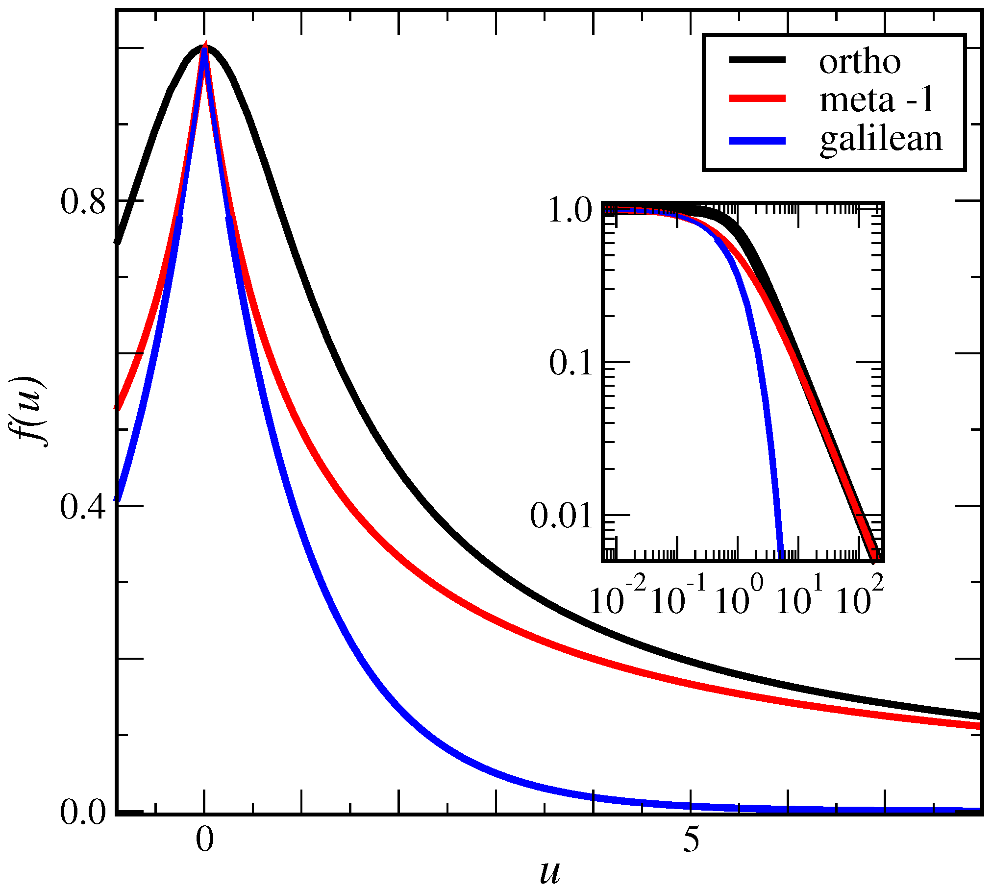
All two-point functions (12), (14) and (16) have indeed the symmetries ${\mathcal{C}}_{12}(t_1,t_2;r,r)={\mathcal{C}}_{21}(t_2,t_1;r,r)$ and ${\mathcal{C}}_{12}(t,t;r_1,r_2)={\mathcal{C}}_{21}(t,t;r_2,r_1)$, under permutation ${\phi }_1\leftrightarrow {\phi }_2$ of the two scaling operators, as physically required for a correlator. The shape of the scaling function of these three two-point function is compared in Figure 3. In particular, the non-analyticity of the meta- and Galilean conformal invariance at $u=0$ is clearly seen, in contrast to ortho-conformal invariance, while for $u\to \infty$, the slow algebraic decay of ortho- and meta-conformal invariance is distinct from the exponential decay of conformal Galilean invariance. This illustrates the variety of possible forms already for $z=1$. Below, we shall find another form of (meta-)conformal invariance, different from all forms displayed in Figure 3.

3. Impossibility of a Local Meta-Conformal Invariance of the dle Process

Can one consider these several variants of conformal invariance, which have $z=1$ and are realised in terms of local first-order differential operators, as a valid dynamical symmetry of the dle process in $1+1$ dimensions ? The answer turns out to be negative:

• The deterministic part of the dle Langevin Equation (1) is distinct from the simple invariant equations $\mathcal{S}\phi =0$ of either ortho- or meta-1-conformal invariance.
  For analogy, consider briefly Schrödinger-invariant systems with a Langevin equation of the form $\mathcal{S}\phi ={\left(2\nu T\right)}^{1/2}\eta$, where $\eta =\frac{\mathrm{d}B}{\mathrm{d}t}$ is a white noise of unit variance, and such that the Schrödinger algebra is a dynamical symmetry of the noise-less equation (deterministic part) $\mathcal{S}{\phi }_0=0$. Then, the Bargman super-selection rules [69] which follow from the combination of spatial translation-invariance and Galilei-invariance with $z=2$, imply exact relations between averages of the full noisy theory and the averages calculated from its deterministic part [70]. In particular, the two-time response function of the full noisy equation $R(t,s;\mathit{r})=R_0(t,s;\mathit{r})$, is identical to the response $R_0$ found when the noise is turned off and computed from the dynamical Schrödinger symmetry [16,70].
  We shall assume here that an analogous result can be derived also for the dle Langevin equation, although this has not yet been done. It seems plausible that such a result should exist, since in the example (5b) and (6b) of the dle process, the two-time response R is independent of T (which characterises the white noise), as it is the case for Schrödinger-invariance.
• The explicit response function (6b) of the dle process is distinct from the predictions (12) , (14) and (16), see also Table 2. The form of the meta-1 conformal two-point function (14), is clearly different for finite values of the scaling variable $v=(r_1-r_2)/(t_1-t_2)$, and similarly for the conformal Galilean case (16). The ortho-conformal two-point function (12) looks to be much closer, with the choice $x_1=\frac{1}{2}$ and the scale factor fixed to $\nu =1$, were it not for the extra factor $\nu (t-s)$.
  On the other hand, the two-time dle-correlator (6a) does not agree with (12) either, but might be similar to a two-point function computed in a semi-infinite space $t\ge 0$, $r\in \mathbb{R}$ with a boundary at $t=0$.

Looking for dynamical symmetries of the deterministic part of the dle Langevin Equation (1), in $1+1$ dimensions, the first test will be the computation of the two-time response function $R(t,s;\mathit{r})$. By contrast, we shall show that the two-time correlator C cannot be found in this way. Indeed, its ‘deterministic’ contribution vanishes: $C_0(t,s;\mathit{r})=0$.

4. Riesz-Feller Fractional Derivative

Formulating (1) in direct space requires the Riesz-Feller fractional derivative [71,72,73] of order α.

Definition 4.

For functions $f(r)$ of a single variable $r\in \mathbb{R}$, the Riesz-Feller derivative, of order α, is

$${\mathrm{\nabla }}_r^{\alpha }f(r):=\frac{{\mathrm{i}}^{\alpha }}{\sqrt{2\pi }}{\int }_{\mathbb{R}}{\mathrm{d}k|k|}^{\alpha }{e}^{\mathrm{i}kr}\widehat{f}(k)=\frac{{\mathrm{i}}^{\alpha }}{2\pi }{\int }_{{\mathbb{R}}^2}\mathrm{d}k\mathrm{d}x{|k|}^{\alpha }{e}^{\mathrm{i}k(r-x)}f(x)$$

(17)

where $\widehat{f}(k)$ denotes the Fourier transform of $f(r)$. For brevity, we often write ${\mathrm{\nabla }}_r={\mathrm{\nabla }}_r^1$ and distinguish it from the standard derivative ${\partial }_r$.

Lemma 1.

([72], Prop. 3.6) Let $f\in H^{\alpha /2}(\mathbb{R})=\left\{f\in L^2(\mathbb{R})\left|{\int }_{\mathbb{R}}\mathrm{d}k|\widehat{f}{(k)|}^2{(1+|k|}^2{)}^{\alpha /2}<\infty \right.\right\}$, a fractional Sobolev space. For $0<\alpha <2$, the Riesz-Feller derivative ${\mathrm{\nabla }}_r^{\alpha }f(r)$ exists.

Lemma 2.

([16] app. J.2, [21]) The following formal properties hold true, where $\alpha ,\beta ,q,\mu$ are constants

$$\begin{array}{ccc}\hfill {\mathrm{\nabla }}_r^{\alpha }{\mathrm{\nabla }}_r^{\beta }f(r)={\mathrm{\nabla }}_r^{\alpha +\beta }f(r)& ,& \left[{\mathrm{\nabla }}_r^{\alpha },r\right]f(r)=\alpha {\partial }_r{\mathrm{\nabla }}_r^{\alpha -2}f(r),{\mathrm{\nabla }}_r^{\alpha }f(\mu r)={|\mu |}^{\alpha }{\mathrm{\nabla }}_{\mu r}^{\alpha }f(\mu r)\hfill \\ \hfill {\mathrm{\nabla }}_r^{\alpha }{e}^{\mathrm{i}qr}={\left(\mathrm{i}|q|\right)}^{\alpha }{e}^{\mathrm{i}qr}& ,& (\widehat{{\mathrm{\nabla }}_r^{\alpha }f(r)})(q)={\left(\mathrm{i}|q|\right)}^{\alpha }\widehat{f}(q),{\mathrm{\nabla }}_r^{2}f(r)={\partial }_r^{2}f(r)\hfill \end{array}$$

(18)

Lemma 2 follows directly from the definition (17). The analogy with the rules of the ordinary derivative ${\partial }_r^n$, with $n\in \mathbb{N}$, applied to exponentials $e^{\mathrm{i}qr}$ and to Fourier transforms, motivated our choice of (complex) normalisation in (17). Later, we shall also need the object ${\partial }_r{\mathrm{\nabla }}_r^{-1}$, which is formally written as

$${\partial }_r{\mathrm{\nabla }}_r^{-1}f(r)=\frac{1}{\sqrt{2\pi }}{\int }_{\mathbb{R}}\mathrm{d}k{e}^{\mathrm{i}kr}\mathrm{sign}(k)\widehat{f}(k)$$

(19)

but is best considered via its Fourier transform, viz. $(\widehat{{\partial }_r{\mathrm{\nabla }}_r^{-1}f(r)})(q)=\mathrm{sign}(q)\widehat{f}(q)$. This is well-defined, since $f\in H^{\alpha /2}(\mathbb{R})\subset L^2(\mathbb{R})$ and because of Plancherel’s theorem. The Fourier transform of $\mathrm{sign}(q)$ is a distribution ([74] [Equation (2.3.17)]).

Corollary 1.

One has the following formal commutator identities

$$\begin{array}{l}\left[{\mathrm{\nabla }}_r,r^n\right]=n{r}^{n-1}{\partial }_r{\mathrm{\nabla }}_r^{-1},\left[r^2{\mathrm{\nabla }}_r,r{\partial }_r\right]=-r^2{\mathrm{\nabla }}_r,\left[r{\partial }_r{\mathrm{\nabla }}_r^{-1},r{\mathrm{\nabla }}_r\right]=-r,\\ \left[{\mathrm{\nabla }}_r,{\partial }_r\right]=\left[r{\partial }_r,r{\mathrm{\nabla }}_r\right]=\left[r,{\partial }_r{\mathrm{\nabla }}_r^{-1}\right]=\left[r^n{\partial }_r,{\partial }_r{\mathrm{\nabla }}_r^{-1}\right]=\left[r^n{\mathrm{\nabla }}_r,{\partial }_r{\mathrm{\nabla }}_r^{-1}\right]=0.\end{array}$$

(20)

Proof. 

Most of these identities are immediate consequences of (17,18). The first one is proven by induction, for all $n\in \mathbb{N}$. We only detail here the computation of the third one. Formally, one has $\left[r{\partial }_r{\mathrm{\nabla }}_r^{-1},r{\mathrm{\nabla }}_r\right]=-r{\left({\partial }_r{\mathrm{\nabla }}_r^{-1}\right)}^2$. Using (19), and its Fourier transform, gives

$${\left({\partial }_r{\mathrm{\nabla }}_r^{-1}\right)}^{2}f(r)={\int }_{\mathbb{R}}\frac{\mathrm{d}k}{\sqrt{2\pi }}{e}^{\mathrm{i}kr}\mathrm{sign}(k)(\widehat{{\partial }_r{\mathrm{\nabla }}_r^{-1}f(r)})(k)={\int }_{\mathbb{R}}\frac{\mathrm{d}k}{\sqrt{2\pi }}{e}^{\mathrm{i}kr}{\left(\mathrm{sign}(k)\right)}^2\widehat{f}(k)=f(r)$$

which establishes the assertion.       ☐

Lemma 3.

[72,75] If $0<\alpha <2$, one has for either $f\in H^{\alpha /2}(\mathbb{R})$ or else $f\in \mathcal{S}(\mathbb{R})$, the Schwartz space of smooth, rapidly decreasing functions, for almost all $r\in \mathbb{R}$

$${\mathrm{\nabla }}_r^{\alpha }f(r)=\frac{1-e^{\mathrm{i}\pi \alpha }}{4\pi \mathrm{i}}\mathrm{\Gamma }(\alpha +1){\int }_{\mathbb{R}}\frac{\mathrm{d}y}{{|y|}^{\alpha +1}}\left[f(r+y)-2f(r)+f(r-y)\right]$$

(21)

If $f\in \mathcal{S}(\mathbb{R})$, ${\mathrm{\nabla }}_r^{\alpha }f(r)$ can be defined beyond the interval $0<\alpha <2$.

5. Non-Local Meta-Conformal Generators

The deterministic part of (1) becomes $\mathcal{S}\phi =\left(-\mu {\partial }_r+{\mathrm{\nabla }}_r\right)\phi =0$, where ${\mu }^{-1}=\mathrm{i}\nu$. Following earlier studies [45], it seems physically reasonable that the Lie algebra of dynamical symmetries should at least contain the generators of time translations $X_{-1}=-{\partial }_t$, dilatations $X_0=-t{\partial }_t-\frac{r}{z}{\partial }_r-\frac{x}{z}$ and space translations $Y_{-1}=-{\partial }_r$. It turns out, however, if one wishes to construct a generator of generalised Galilei transformations as a dynamical symmetry, the non-local generator $-{\mathrm{\nabla }}_r$ automatically arises, see below and ([16], Chapter 5.3). It is still an open problem how to close these generators into a Lie algebra, for $z\ne 2$ and beyond the examples listed above in Section 2.

This difficulty motivates us to start with the choice of a non-local spatial translation operator $Y_{-1}=-{\mu }^{-1}{\mathrm{\nabla }}_r$. Here indeed, a closed Lie algebra can be found.

Proposition 1.

[21] Define the following generators

$$\begin{array}{ccc}\hfill X_{-1}& =& -{\partial }_t,X_0=-t{\partial }_t-r{\partial }_r-x,X_1=-t^2{\partial }_t-2tr{\partial }_r-\mu r^2{\mathrm{\nabla }}_r-2xt-2\gamma r{\partial }_r{\mathrm{\nabla }}_r^{-1}\hfill \\ \hfill Y_{-1}& =& -\frac{1}{\mu }{\mathrm{\nabla }}_r,Y_0=-\frac{1}{\mu }t{\mathrm{\nabla }}_r-r{\partial }_r-\frac{\gamma }{\mu },Y_1=-\frac{1}{\mu }{t}^2{\mathrm{\nabla }}_r-2tr{\partial }_r-\mu r^2{\mathrm{\nabla }}_r-2\frac{\gamma }{\mu }t-2\gamma r{\partial }_r{\mathrm{\nabla }}_r^{-1}\hfill \end{array}$$

(22)

where the constants $x=x_{\phi }$ and $\gamma ={\gamma }_{\phi }$, respectively, are the scaling dimension and rapidity of the scaling operator $\phi =\phi (t,r)$ on which these generators act. The six generators (22) obey the commutation relations of a meta-conformal Lie algebra, isomorphic to $\mathfrak{sl}(2,\mathbb{R})\oplus \mathfrak{sl}(2,\mathbb{R})$

$$\left[X_n,X_m\right]=(n-m)X_{n+m},\left[X_n,Y_m\right]=(n-m)Y_{n+m},\left[Y_n,Y_m\right]=(n-m)Y_{n+m}$$

(23)

Proposition 2.

[21] The generators (22) obey the commutators

$$\left[\mathcal{S},Y_n\right]\phi =\left[\mathcal{S},X_{-1}\right]\phi =0,\left[\mathcal{S},X_0\right]\phi =-\mathcal{S}\phi ,\left[\mathcal{S},X_1\right]\phi =-2t\mathcal{S}\phi +2(\mu x-\gamma )\phi$$

(24)

with the operator $\mathcal{S}=-\mu {\partial }_t+{\mathrm{\nabla }}_r$ and thus form a Lie algebra of meta-conformal dynamical symmetries (of the deterministic part) $\mathcal{S}\phi =0$ of the dle Langevin Equation (1), if only $\gamma =x\mu$.

The non-local generators $X_1,Y_{0,1}$ in (22) do not generate simple local changes of the coordinates $(t,r)$, in contrast to all examples of Section 2. Finding a clear geometrical interpretation of the generators (22) remains an open problem.

This meta-conformal symmetry algebra can be considerably enlarged.

Proposition 3.

Consider the generators (22) and furthermore define

$$Z_{-1}=-\frac{1}{\mu }{\partial }_r,Z_0=-\frac{1}{\mu }t{\partial }_r-r{\mathrm{\nabla }}_r-\frac{\gamma }{\mu }{\partial }_r{\mathrm{\nabla }}_r^{-1},Z_1=-\frac{1}{\mu }{t}^2{\partial }_r-2tr{\mathrm{\nabla }}_r-\mu r^2{\partial }_r-2\frac{\gamma }{\mu }t{\partial }_r{\mathrm{\nabla }}_r^{-1}-2\gamma r$$

(25)

These generators are dynamical symmetries of the dle Langevin equation, since $\left[\mathcal{S},Z_n\right]=0$ and they extend the meta-conformal Lie algebra (23) as follows

$$\left[X_n,Z_m\right]=(n-m)Z_{n+m},\left[Y_n,Z_m\right]=(n-m)Z_{n+m},\left[Z_n,Z_m\right]=(n-m)Y_{n+m}$$

(26)

Although $Z_{-1}$ generates local spatial translations, the transformations obtained from $Z_{0,1}$ are non-local. In what follows, we write $\xi :=\gamma /\mu$ for the second, independent scaling dimension of φ.

Corollary 2.

Define the generators $B_n^{\pm }=\frac{1}{2}\left(Y_n\pm Z_n\right)$, $n\in \{-1,0,1\}$. Then the non-vanishing commutators of the Lie algebra (23) and (26) take the form

$$\left[X_n,X_m\right]=(n-m)X_{n+m},\left[X_n,B_m^{\pm }\right]=(n-m)B_{n+m}^{\pm },\left[B_n^{\pm },B_m^{\pm }\right]=(n-m)B_{n+m}^{\pm }$$

(27)

The $B_n^{\pm }$ are dynamical symmetries of thedleprocess, since $\left[\mathcal{S},B_n^{\pm }\right]=0$.

Corollary 3.

Define the generators $A_n=X_n-\left(B_n^{+}+B_n^{-}\right)=X_n-Y_n$, $n\in \{-1,0,1\}$. Then the non-vanishing commutators of the Lie algebra (27) are

$$\left[A_n,A_m\right]=(n-m)A_{n+m},\left[B_n^{\pm },B_m^{\pm }\right]=(n-m)B_{n+m}^{\pm }$$

(28)

This Lie algebra of dynamical symmetries of the deterministic part of the dle Langevin Equation (1) is isomorphic to the direct sum $\mathfrak{sl}(2,\mathbb{R})\oplus \mathfrak{sl}(2,\mathbb{R})\oplus \mathfrak{sl}(2,\mathbb{R})$.

In this last choice of basis, all generators contain non-local terms. Their form, in Corollary 3, is suggestive for the explicit construction of an infinite-dimensional extension of the above Lie algebra.

Proposition 4.

Construct the generators, for all $n\in \mathbb{Z}$ and $x,\xi$ constants

$$\begin{array}{ccc}\hfill A_n& =& -t^{n+1}\left({\partial }_t-{\mathrm{\nabla }}_r\right)-(n+1)\left(x-\xi \right)t^n\hfill \\ \hfill B_n^{\pm }& =& -\frac{1}{2}{\left(t\pm r\right)}^{n+1}\left({\mathrm{\nabla }}_r\pm {\partial }_r\right)-\frac{n+1}{2}\xi {\left(t\pm r\right)}^n\left(1\pm {\partial }_r{\mathrm{\nabla }}_r^{-1}\right)\hfill \end{array}$$

(29)

Their non-vanishing commutators are given by (28), for $n,m\in \mathbb{Z}$. Their Lie algebra is isomorphic to the direct sum of three Virasoro algebras with vanishing central charges. They are also dynamic symmetries of the deterministic equation $\mathcal{S}\phi =\left(-{\partial }_t+{\mathrm{\nabla }}_r\right)\phi =0$ of dle process, provided that $x=\xi$, because of the commutators

$$\left[\mathcal{S},A_n\right]=-(n+1)t^n\mathcal{S}+(n+1)n\left(x-\xi \right)t^{n-1},\left[\mathcal{S},B_n^{\pm }\right]=0$$

(30)

Proof. 

For $n=\pm 1,0$, the generators (29) are those given above in (22) and (25), using $\xi =\gamma /\mu$ and rescaling $\mu \mapsto 1$. One generalises the first identity (20) in the Corollary 1 to the following form, with $n\in \mathbb{N}$

$$\left[{\mathrm{\nabla }}_r,{\left(\alpha \pm r\right)}^n\right]=\pm n{\left(\alpha \pm r\right)}^{n-1}{\partial }_r{\mathrm{\nabla }}_r^{-1}$$

where α is a constant. The assertions now follow by direct formal calculations, using (18) and (20). ☐

This is the dle-analogue of the ortho- and meta-1 conformal invariances, respectively, of the Laplace equation and of simple ballistic transport, as treated in Examples 3 and 4. In Table 3, it is called “meta-2 conformal”. It clearly appears that both local and non-local spatial translations are needed for realising the full dynamical symmetry of the dle process, which we call erosion-Virasoro algebra and denote by $\mathfrak{ev}$. The infinite-dimensional Lie algebra $\mathfrak{ev}$ is built from three commuting Virasoro algebras (obviously, the maximal finite-dimensional Lie sub-algebra is $\mathfrak{sl}(2,\mathbb{R})\oplus \mathfrak{sl}(2,\mathbb{R})\oplus \mathfrak{sl}(2,\mathbb{R})$). The scaling operators $\phi =\phi (t,r)$ on which these generators act are characterised by two independent scaling dimensions $x=x_{\phi }$ and $\xi ={\xi }_{\phi }$. By analogy with conformal Galilean invariance [76], one expects that three independent central charges of the Virasoro type should appear if the algebra (28) will be quantised. Additional physical constraints (e.g. unitarity) may reduce the number of independent central charges.

6. Ward Identities for Co-Variant Quasi-Primary n-Point Functions

A basic application of dynamic time-space symmetries is the derivation of co-variant n-point functions. Adapting the corresponding definition from (ortho-)conformal invariance [1], a scaling operator $\phi =\phi (t,r)$ is called quasi-primary, if it transforms co-variantly under the action of the generators of the maximal finite-dimensional sub-algebra of $\mathfrak{ev}$. A primary scaling operator transforms co-variantly under the action of all generators of $\mathfrak{ev}$. In this work, we consider examples of n-point functions of quasi-primary scaling operators.

In the physical context of non-equilibrium dynamics, such n-point functions can either be correlators, such as $\langle \phi (t,r)\phi (t^{\prime },r^{\prime })\rangle$, or response functions $\langle \phi (t,r)\tilde{\phi }(t^{\prime },0)\rangle ={\left.\frac{\delta \langle \phi (t,r)\rangle }{\delta j(t^{\prime },0)}\right|}_{j=0}$, which can be formally rewritten as a correlator by using the formalism of Janssen-de Dominicis theory [17] which defines the response operator $\tilde{\phi },$ conjugate to the scaling operator φ.

Proceeding in analogy with ortho-conformal and Schrödinger-invariance [1,16,43,44,77], the quasi-primary $\mathfrak{ev}$-Ward identities are obtained from the explicit form of the Lie algebra generators (22) and (25), generalised to n-body generators. In order to do so, we assign a signature $\epsilon =\pm 1$ to each scaling operator [21]. We choose the convention that ${\epsilon }_i=+1$ for scaling operators ${\phi }_i$ and ${\epsilon }_i=-1$ for response operators ${\tilde{\phi }}_i$. In order to prepare a later application to the conformal Galilean algebra, to be obtained from a Lie algebra contraction, we also multiply the generators $Y_i,Z_i$ by the scale factor μ. The n-body generators then read

$$\begin{array}{ccc}\hfill X_{-1}=X_{-1}^{\left[n\right]}& =& {\displaystyle \sum _i}\left[-{\partial }_i\right],X_0=X_0^{\left[n\right]}={\displaystyle \sum _i}\left[-t_i{\partial }_i-r_i{D}_i-x_i\right]\hfill \\ \hfill X_1=X_1^{\left[n\right]}& =& {\displaystyle \sum _i}\left[-t_i^2{\partial }_i-2t_i{r}_i{D}_i-\mu {\epsilon }_i{r}_i^2{\mathrm{\nabla }}_i-2x_i{t}_i-2\mu {\xi }_i{\epsilon }_i{r}_i{D}_i{\mathrm{\nabla }}_i^{-1}\right]\hfill \\ \hfill Y_{-1}=Y_{-1}^{\left[n\right]}& =& {\displaystyle \sum _i}\left[-{\epsilon }_i{\mathrm{\nabla }}_i\right],Y_0=Y_0^{\left[n\right]}={\displaystyle \sum _i}\left[-{\epsilon }_i{t}_i{\mathrm{\nabla }}_i-\mu r_i{D}_i-\mu {\xi }_i\right]\hfill \\ \hfill Y_1=Y_1^{\left[n\right]}& =& {\displaystyle \sum _i}\left[-{\epsilon }_i\left(t_i^2+{\mu }^2{r}_i^2\right){\mathrm{\nabla }}_i-2\mu t_i{r}_i{D}_i-2\mu {\xi }_i{t}_i-2{\mu }^2{\xi }_i{\epsilon }_i{r}_i{D}_i{\mathrm{\nabla }}_i^{-1}\right]\hfill \\ \hfill Z_{-1}=Z_{-1}^{\left[n\right]}& =& {\displaystyle \sum _i}\left[-D_i\right],Z_0=Z_0^{\left[n\right]}={\displaystyle \sum _i}\left[-t_i{D}_i-{\epsilon }_i{r}_i{\mathrm{\nabla }}_i-\mu {\xi }_i{D}_i{\mathrm{\nabla }}_i^{-1}\right]\hfill \\ \hfill Z_1=Z_1^{\left[n\right]}& =& {\displaystyle \sum _i}\left[-\left(t_i^2+{\mu }^2{r}_i^2\right)D_i-2{\epsilon }_i\mu t_i{r}_i{\mathrm{\nabla }}_i-2\mu {\xi }_i{r}_i-2\mu {\xi }_i{\epsilon }_i{t}_i{D}_i{\mathrm{\nabla }}_i^{-1}\right]\hfill \end{array}$$

(31)

with the short-hands ${\partial }_i=\frac{\partial }{\partial t_i}$, $D_i=\frac{\partial }{\partial r_i}$ and ${\mathrm{\nabla }}_i={\mathrm{\nabla }}_{r_i}$. It can be checked that the generators (31) obey the meta-conformal Lie algebra of the dle process. Define the $(n+m)$-point function

$$\begin{array}{ccc}\hfill {\mathcal{C}}_{n,m}& =& {\mathcal{C}}_{n,m}(t_1,\dots ,t_{n+m};r_1,\dots ,r_{n+m})\hfill \\ & =& 〈{\phi }_1(t_1,r_1)\cdots {\phi }_n(t_n,r_n){\tilde{\phi }}_{n+1}(t_{n+1},r_{n+1})\cdots {\tilde{\phi }}_{n+m}(t_{n+m},r_{n+m})〉\hfill \end{array}$$

(32)

of quasi-primary scaling and response operators. Their co-variance is expressed through the quasi-primary Ward identities, for $k=\pm 1,0$

$$X_k^{[n+m]}{\mathcal{C}}_{n,m}=Y_k^{[n+m]}{\mathcal{C}}_{n,m}=Z_k^{[n+m]}{\mathcal{C}}_{n,m}=0,$$

(33)

The solution of this set of (linear) differential equations gives the sought $(n+m)$-point function ${\mathcal{C}}_{n,m}$.

7. Co-Variant Two-Time Correlators and Responses

In order to illustrate the procedure outlined in section 6, we shall apply it to the two-point functions.

Proposition 5.

Any two-point correlator ${\mathcal{C}}_{2,0}(t_1,t_2;r_1,r_2)=\langle {\phi }_1(t_1,r_1){\phi }_2(t_2,r_2)\rangle$, built from $\mathfrak{ev}$-quasi-primary scaling operators ${\phi }_i$, vanishes.

Proof. 

Time-translation-invariance, expressed by $X_{-1}{\mathcal{C}}_{2,0}=0$, implies that ${\mathcal{C}}_{2,0}={\mathcal{C}}_{2,0}(t;r_1,r_2)$, with $t=t_1-t_2$. Invariance under both non-local and local space-translations gives $Y_{-1}{\mathcal{C}}_{2,0}=Z_{-1}{\mathcal{C}}_{2,0}=0$. In Fourier space, this becomes

$$\left({\epsilon }_1|q_1|+{\epsilon }_2|q_2|\right){\widehat{\mathcal{C}}}_{2,0}(t;q_1,q_2)=0,\left(q_1+q_2\right){\widehat{\mathcal{C}}}_{2,0}(t;q_1,q_2)=0$$

where the signatures are both positive, viz. ${\epsilon }_1={\epsilon }_2=+1$. The only solution is ${\widehat{\mathcal{C}}}_{2,0}(t;q_1,q_2)=0$.  ☐

Recall that the dynamical symmetry of the $\mathfrak{ev}$ algebra is only a symmetry of the deterministic part of the dle Langevin equation (1), which corresponds to $T=0$. The vanishing of ${\mathcal{C}}_{2,0}$ is seen explicitly in the exact dle-correlator (5a,6a), which indeed vanishes as $T\to 0$. This result of the dle process is analogous to what is found for Schrödinger-invariant systems [16,77], where it follows from a Bargman superselection rule [69]. Still, this does not mean that symmetry methods could only predict vanishing correlators. For example, in Schrödinger-invariant systems, correlators with $T\ne 0$ can be found from certain integrals of higher n-point responses [16,70]. For a simple illustration in the noisy Edwards-Wilkinson equation, see [78]. We conjecture that an analogous procedure might work for the dle process and hope to return to this elsewhere.

We now concentrate on the two-time response function $\mathcal{R}=\mathcal{R}(t_1,t_2;r_1,r_2)={\mathcal{C}}_{1,1}(t_1,t_2;r_1,r_2)$. Time-translation-invariance, which imposes $X_{-1}\mathcal{R}=0$, implies that $\mathcal{R}=\mathcal{R}(t;r_1,r_2)$, with $t=t_1-t_2$. Invariance under non-local and local space-translations now give (in Fourier space)

$${\epsilon }_1\left(|q_1|-|q_2|\right)\widehat{\mathcal{R}}(t;q_1,q_2)=0,\left(q_1+q_2\right)\widehat{\mathcal{R}}(t;q_1,q_2)=0$$

since the signatures are now ${\epsilon }_1=-{\epsilon }_2=+1$. Here, a non-vanishing solution is possible and we can write $\mathcal{R}=F(t,r)$, with $r=r_1-r_2$.

Proposition 6.

The $\mathfrak{ev}$-covariant two-point response function $\mathcal{R}={\mathcal{C}}_{1,1}$ from (32) satisfies the scaling form $\mathcal{R}=\langle {\phi }_1(t,r){\tilde{\phi }}_2(0,0)\rangle =t^{-2x}f(v)$, with the scaling variable $v=r/t$. If the scaling function $f(v)$ obeys the following two conditions, with the abbreviations $x=\frac{1}{2}(x_1+x_2)$ and $\xi =\frac{1}{2}({\xi }_1+{\xi }_2)$,

$$\left({\epsilon }_1{\mathrm{\nabla }}_v+\mu v{\partial }_v+2\mu \xi \right)f(v)=0,(x_1-x_2)\left({\epsilon }_1{\mathrm{\nabla }}_v+\mu v{\partial }_v+\mu \right)f(v)=0.$$

(34)

and the constraint ${\xi }_1-{\xi }_2=x_1-x_2$ holds true, then all quasi-primary Ward identities are satisfied.

The conditions (34) come from the deterministic part of the dle Langevin Equation (1) and do not contain T. This is consistent with the T-independence of the exact dle-response function (5b) and (6b). A fuller justification, analogous to the derivation of the Bargman superselection rules of Schrödinger-invariance [70,77], is left as an open problem, for future work.

Proof. 

Denote by $x_i$ and ${\xi }_i$ (with $i=1,2$), the two scaling dimensions of the scaling operator ${\phi }_1$ and of the response operator ${\tilde{\phi }}_2$, respectively. Time-translation-invariance and non-local and local space-translation-invariances produced the form $\mathcal{R}=F(t,r)$, with $t=t_1-t_2$, $r=r_1-r_2$ and the signatures ${\epsilon }_1=-{\epsilon }_2=+1$. The other six Ward identities lead to the conditions, using (18)

$$\begin{array}{cc}\hfill \left[-t{\partial }_t-r{\partial }_r-x_1-x_2\right]F& =0\hfill \end{array}$$

(35a)

$$\begin{array}{cc}\hfill \left[-t{\epsilon }_1{\mathrm{\nabla }}_r-\mu r{\partial }_r-\mu {\xi }_1-\mu {\xi }_2\right]F& =0\hfill \end{array}$$

(35b)

$$\begin{array}{cc}\hfill \left[-t{\partial }_r-\mu {\epsilon }_{1}r{\mathrm{\nabla }}_r-\mu ({\xi }_1+{\xi }_2){\epsilon }_1{\partial }_r{\mathrm{\nabla }}_r^{-1}\right]F& =0\hfill \end{array}$$

(35c)

$$\begin{array}{cc}\hfill \left[-t^2{\partial }_t-2tr{\partial }_r-\mu r^2{\epsilon }_1{\mathrm{\nabla }}_r-2x_{1}t-2\mu {\xi }_1{\epsilon }_{1}r{\partial }_r{\mathrm{\nabla }}_r^{-1}\right]F& =0\hfill \end{array}$$

(35d)

$$\begin{array}{cc}\hfill \left[-t^2{\epsilon }_1{\mathrm{\nabla }}_r-2\mu tr{\partial }_r-{\mu }^2{\epsilon }_1{r}^2{\mathrm{\nabla }}_r-2\mu {\xi }_{1}t-2{\mu }^2{\xi }_1{\epsilon }_{1}r{\partial }_r{\mathrm{\nabla }}_r^{-1}\right]F& =0\hfill \end{array}$$

(35e)

$$\begin{array}{cc}\hfill \left[-t^2{\partial }_r-2\mu {\epsilon }_{1}tr{\mathrm{\nabla }}_r-{\mu }^2{r}^2{\partial }_r-2{\mu }^2{\xi }_{1}r-2\mu {\xi }_1{\epsilon }_{1}t{\partial }_r{\mathrm{\nabla }}_r^{-1}\right]F& =0\hfill \end{array}$$

(35f)

Herein, Equation (35d) is obtained by using Equations (35a) and (35c), and Equations (35e) and (35f) are obtained by using (35b) and (35c). Actually, because of the identity

$$\begin{array}{ccc}\hfill \left[-t{\partial }_r-\mu {\epsilon }_{1}r{\mathrm{\nabla }}_r-2\mu \xi {\epsilon }_1{\partial }_r{\mathrm{\nabla }}_r^{-1}\right]F& =& {\epsilon }_1\left[-t{\epsilon }_1{\mathrm{\nabla }}_r{\partial }_r{\mathrm{\nabla }}_r^{-1}-\mu r{\mathrm{\nabla }}_r^2{\mathrm{\nabla }}_r^{-1}-2\mu \xi {\partial }_r{\mathrm{\nabla }}_r^{-1}\right]F\hfill \\ & =& {\epsilon }_1{\partial }_r{\mathrm{\nabla }}_r^{-1}\left[-{\epsilon }_{1}t{\mathrm{\nabla }}_r-\mu r{\partial }_r-2\mu \xi \right]F\hfill \end{array}$$

the condition $Y_{0}F=0$, Equation (35b), implies $Z_{0}F=0$, Equation (35c). Since ${\left({\partial }_r{\mathrm{\nabla }}_r^{-1}\right)}^{2}f(r)=f(r)$, see the Corrollary 1, the converse also holds true. Next, Equation (35d) can be simplified further: multiply Equation (35a) with t and subtract it from (35d), which gives

$$\left[-tr{\partial }_r-\mu {\epsilon }_1{r}^2{\mathrm{\nabla }}_r-(x_1-x_2)t-2\mu {\xi }_1{\epsilon }_{1}r{\partial }_r{\mathrm{\nabla }}_r^{-1}\right]F=0$$

(36)

Then multiply (35c) with r and substract it from (36). This gives the condition

$$\left[\left(x_1-x_2\right)t+\mu \left({\xi }_1-{\xi }_2\right){\epsilon }_{1}r{\partial }_r{\mathrm{\nabla }}_r^{-1}\right]F=0$$

(37)

Similarly, simplify Equation (35e): multiply (35b) by t and subtract from (35e), then multiply (36) by μ and subtract as well. This gives

$$\mu \left[\left({\xi }_1-{\xi }_2\right)-\left(x_1-x_2\right)\right]tF=0$$

Unless $F\sim \delta (t)$ is a distribution, this gives the constraint ${\xi }_1-{\xi }_2=x_1-x_2$. Finally, Equation (35f) is simplified by multiplying first (35c) with t and subtracting and then multiplying (35b) with r and subtracting as well. This leads to $({\xi }_1-{\xi }_2)\left[\mu r+{\epsilon }_{1}t{\partial }_r{\mathrm{\nabla }}_r^{-1}\right]F=0$. Since in the proof of the Corollary 1, we have seen that ${\left({\partial }_r{\mathrm{\nabla }}_r^{-1}\right)}^{2}f(r)=f(r)$, this can be rewritten as follows: $({\xi }_1-{\xi }_2){\epsilon }_1\left({\partial }_r{\mathrm{\nabla }}_r^{-1}\right)\left[{\epsilon }_1\mu r{\partial }_r{\mathrm{\nabla }}_r^{-1}+t\right]F=0$. Taking the constraint into account, the last condition can be combined with (37) into the single equation

$$\left(x_1-x_2\right)\left[t+\mu {\epsilon }_{1}r{\partial }_r{\mathrm{\nabla }}_r^{-1}\right]F=0$$

(38)

The form of F is now fixed by the three equations (35a,35b,38) and the constraint has to be obeyed.

Equation (35a) implies the scaling form $F=t^{-2x}f(r/t)$. Inserting this into (35b) produces, with the help of (18), the first of the Equations (34). Finally, inserting the scaling form for F into (38) gives $(x_1-x_2)\left(1+\mu {\epsilon }_{1}v{\partial }_v{\mathrm{\nabla }}_v^{-1}\right)f(v)=0$. Since it is not immediately obvious if that condition is consistent with the first Equation (34), we rephrase it as follows: use the commutator $\left[v{\partial }_v,{\mathrm{\nabla }}_v^{-1}\right]={\mathrm{\nabla }}_v^{-1}$ to write formally $v{\partial }_v{\mathrm{\nabla }}_v^{-1}={\mathrm{\nabla }}_v^{-1}+{\mathrm{\nabla }}_v^{-1}\left(v{\partial }_v\right)$. Then, apply ${\mathrm{\nabla }}_v$ to the last condition on $f(v)$ derived from (38), in order to rewrite it as follows

$${\mathrm{\nabla }}_v{\mathrm{\nabla }}_v^{-1}\left[\left(x_1-x_2\right)\left({\epsilon }_1{\mathrm{\nabla }}_v+\mu v{\partial }_v+\mu \right)\right]f(v)=0$$

and this equation is obeyed if the second Equation (34) holds true. We have found a sufficient set of conditions to satisfy all nine dle-quasi-primary Ward identities for $\mathcal{R}={\mathcal{C}}_{1,1}$.         ☐

The two conditions in Equation (34) are compatible in two distinct cases:

Case A:

$2\xi =1$. Then $\left({\epsilon }_1{\mathrm{\nabla }}_v+\mu v{\partial }_v+\mu \right)f(v)=0$ and $x_1\ne x_2$ is still possible.

Case B:

$x_1=x_2$. Then ${\xi }_1={\xi }_2$ and $\left({\epsilon }_1{\mathrm{\nabla }}_v+\mu v{\partial }_v+2\mu \xi \right)f(v)=0$.

We must also compare the differential operator $\mathcal{S}=-\mu {\partial }_t+{\mathrm{\nabla }}_r$ with the dle Langevin Equation (1). Taking into account the normalisation in the definition of the Riesz-Feller derivative, we find ${\mu }^{-1}=\mathrm{i}\nu$. Physically, one should require $\nu >0$ in order that the correlators and responses vanish for large momenta $|q|\to \infty$.

Proposition 7.

The $\mathfrak{ev}$-co-variant two-time response function ${\mathcal{R}}_{12}(t,r)=F(t,r)$ has the form

$$\begin{array}{ccc}\hfill F(t,r)& =& F_A{\delta }_{{\xi }_1+{\xi }_2,1}{\delta }_{{\xi }_1-{\xi }_2,x_1-x_2}{t}^{1-x_1-x_2}\frac{\nu t}{{\nu }^2{t}^2+r^2}\hfill \\ & & +F_B{\delta }_{x_1,x_2}{\delta }_{{\xi }_1,{\xi }_2}{t}^{1+\psi -2x_1}{\left({\nu }^2{t}^2+r^2\right)}^{-(\psi +1)/2}cos\left((\psi +1)arctan\left(\frac{r}{\nu t}\right)-\frac{\pi \psi }{2}\right)\hfill \end{array}$$

(39)

where $\psi =({\xi }_1+{\xi }_2)-1$ is assumed real, $F_{A,B}$ are normalisation constants and the convention ${\epsilon }_1=+1$ is admitted.

Proof. 

Both cases can be treated in the same way. The first Equation (34) becomes in Fourier space

$$\left[\mathrm{i}{\epsilon }_1|q|-\mu q{\partial }_q+\mu (2\xi -1)\right]\widehat{f}(q)=0$$

In case A, the constant term vanishes, while it is non-zero in case B. The solution reads

$$\widehat{f}(q)={\widehat{f}}_0{q}^{2\xi -1}exp\left(\mathrm{i}{\epsilon }_1|q|/\mu \right)={\widehat{f}}_0{q}^{2\xi -1}exp\left(-{\epsilon }_1\nu |q|\right)$$

where ${\widehat{f}}_0$ is a normalisation constant and we can now adopt ${\epsilon }_1=+1$. We also introduced the constant ν from the dle Langevin Equation (1) to illustrate that $\widehat{f}(q)\to 0$ for $|q|$ large when ν is positive. Both cases A and B produce valid solutions of the linear Equations (34). Therefore, the general solution should be a linear superposition of both cases. Carrying out the inverse Fourier transforms is straightforward.          ☐

Remark 3.

Propositions 4 and 7 contain the assertions in the Theorem 1, which are also listed in Table 3. Proposition 5 proves the statement in Remark 2. We had already mentioned in Section 1 (Remark 1), that if we restrict to case A and take $x=x_1=x_2=\frac{1}{2}$ and $\nu >0$, the resulting two-time response $F(t,r)=F_0{t}^{1-2x}{\epsilon }_1\nu t/({\nu }^2{t}^2+r^2)$, with $t=t_1-t_2$ and $r=r_1-r_2$, reproduces the exact solution (6b). We stress that no choice of $x_1$ will make the ortho-conformal prediction (12) compatible with (6b).

This is the main conceptual point of this work: The non-local representation (29) of the meta-conformal algebra $\mathfrak{ev}$ is necessary to reproduce the correct scaling behaviour of the non-stationary response of the dle process.

The non-local meta-2 conformal invariance produces the response function $\mathcal{R}={\mathcal{C}}_{1,1}$, whereas all local ortho-, Galilean and meta-conformal invariances yielded a correlator ${\mathcal{C}}_{2,0}$.

The main result (8) and (39) on the shape of the meta-2-conformal response can be cast into the scaling form $t^{x_1+x_2}{\mathcal{R}}_{12}(t,r)=f(r/t)$, with the explicit scaling function

$$f(u)=\frac{{\left(1+u^2\right)}^{-1}+\rho {\left(1+u^2\right)}^{-{\xi }_1}sin\left(\pi {\xi }_1-2{\xi }_{1}arctanu\right)}{1+\rho sin\pi {\xi }_1}.$$

(40)

We see that the first scaling dimensions $x_1,x_2$ merely arrange the data collapse, while the form of the scaling functions only depends on the second scaling dimension ${\xi }_1={\xi }_2$ and the amplitude ratio ρ (the exact solution (6b) of the dle-process corresponds to $\rho =0$). The normalisation is chosen such that $f(0)=1$. For ${\xi }_1=\frac{1}{2}$, we simply have $f(u)={(1+u^2)}^{-1}$. In Figure 4, several examples of the shape of $f(u)$ are shown. Clearly, these are quite distinct from all the examples of ortho-, meta-1- and Galilean-conformal invariance, displayed above in Figure 3.

Remark 4.

By analogy with Schrödinger-invariance, we conjecture that the fluctuation-dominated correlators should be obtained from certain time-space integrals of higher n-point responses [16,70]. Working with the quantum chain representation of the terrace-step-kink model, Karevski and Schütz have calculated the stationary two-point correlator of the densities, which in our terminology correspond to the slopes $u(t,r)={\partial }_{r}h(t,r)$. They find [10]

$$C(t,r)=C_A{t}^{-2}\frac{1-{\zeta }^2}{{(1+{\zeta }^2)}^2}+C_B{t}^{-\psi }\frac{cos\left[2(q^{*}r-\omega t)\right]}{{(1+{\zeta }^2)}^{\psi }}$$

(41)

with the scaling variable $\zeta =(r-v_{c}t)/(\nu t)$, where $v_c$ is the global velocity of the interface, $\psi \ge \frac{1}{2}$ is a real parameter and $C_{A,B}$ are normalisation constants. The structure of their result is qualitatively very close to the form (8) and (39) for the two-time response of the $\mathfrak{ev}$-algebra, in the sense that it contains a dominant and monotonous term and a non-dominant and oscillatory one. Indeed, it can be checked that from the exact height-height correlator (5a) and (6a) this first term in (41) is recovered by computing the correlator $\langle u(t,r)u(0,0)\rangle$ of the densities $u={\partial }_{r}h$. We interpret this as an encouraging signal that it should be possible to find the correlators from the $\mathfrak{ev}$ as well, by drawing on the analogies with Schrödinger-invariance. The first step in this direction would be the derivation of an analogue of a Bargman superselection rule, which is work in progress.

Remark 5.

The consequences of the choice of the fractional derivative are difficult to appreciate in advance and largely remain a matter of try and error. Our choice of the Riesz-Feller derivative was suggested that in this way the Lie algebra becomes a dynamical symmetry of the dle process. In the past, we had also worked [16,45] with an extension of the Riemann-Liouville derivative by distributional terms [74]. For dynamical exponents $z\ne 1,2$, this leads to a strong oscillatory behaviour of the response functions which appears to be physically undesirable. We consider the success of the simple case study of the dle process treated here as suggestive for future investigations.

Corollary 4.

In the limit $\mu \to 0$ (or $\nu \to \infty$) the Lie algebra $\mathfrak{ev}$ can be contracted into the algebra

$$\left[X_n,X_m\right]=(n-m)X_{n+m},\left[X_n,B_m^{\pm }\right]=(n-m)B_{n+m}^{\pm }$$

(42)

with $n,m\in \mathbb{Z}$ and with the explicit generators

$$\begin{array}{ccc}\hfill X_n& =& -t^{n+1}{\partial }_t-(n+1)t^{n}r{\partial }_r-(n+1)x{t}^n-n(n+1)\epsilon \gamma t^{n-1}r{\partial }_r{\mathrm{\nabla }}_r^{-1}\hfill \\ \hfill B_n^{\pm }& =& -\frac{1}{2}{t}^{n+1}\left(\epsilon {\mathrm{\nabla }}_r\pm {\partial }_r\right)-\frac{1}{2}(n+1)\gamma t^n\left(1\pm \epsilon {\partial }_r{\mathrm{\nabla }}_r^{-1}\right)\hfill \end{array}$$

(43)

where $\epsilon =\pm 1$ is the signature and $x=x_{\phi }$ and $\gamma ={\gamma }_{\phi }$ are the scaling dimension and the rapidity of the scaling operator on which these generators act. The co-variant quasi-primary two-point correlator ${\mathcal{C}}_{2,0}=0$, whereas the co-variant quasi-primary two-point response $\mathcal{R}={\mathcal{C}}_{1,1}$ is, with the normalisation constant ${\mathcal{R}}_0$

$$\mathcal{R}(t,r)={\delta }_{x_1,x_2}{\delta }_{{\gamma }_1,{\gamma }_2}{\mathcal{R}}_0{t}^{-2x_1}exp\left(-2\left|\frac{{\gamma }_{1}r}{t}\right|\right).$$

(44)

The algebra (42), which one might call meta-conformal Galilean algebra, contains the conformal Galilean algebra as a sub-algebra, although the generators (43) are in general non-local, in contrast with those in Equation (15). However, the co-variant two-point function is here a response, and not a correlator.

Proof. 

In order to carry out the contraction on the generators (29), where $X_n=A_n+B_n^{+}+B_n^{-}$, we first change coordinates $r\mapsto \mu r$, let ${\xi }_i={\gamma }_i/\mu$ and rescale the generators $B_n^{\pm }\mapsto \mu B_n^{\pm }$. Then the last commutator in (27) becomes $\left[B_n^{\pm },B_m^{\pm }\right]=\mu (n-m)B_{n+m}^{\pm }$. Taking the limit $\mu \to 0$ produces the generators (43) and the commutators (42) immediately follow. The Ward identities for the finite-dimensional sub-algebra are written down as before and ${\mathcal{C}}_{2,0}=0$ follows. For the response function, going again through the proof of the proposition 7 and recalling that ${\mu }^{-1}=\mathrm{i}\nu$, we see that case A in (39) does not have a non-vanishing limit as $\nu \to \infty$. For case B, consider the scaling form $\mathcal{R}(t,r)=t^{-2x_1}f(r/t)$, with the scaling function $f(v)$ written as

$$f(v)=f_0\left[{\left(\frac{{\epsilon }_1}{\mathrm{i}\mu }-iv\right)}^{-\psi -1}+e^{\mathrm{i}\pi \psi }{\left(\frac{{\epsilon }_1}{\mathrm{i}\mu }+iv\right)}^{-\psi -1}\right]$$

and $\psi +1=2{\gamma }_1/\mu$. If ${\gamma }_1>0$, the first term ${\left(-\mathrm{i}/\mu -\mathrm{i}v\right)}^{-\psi -1}={\left(\mathrm{i}\mu \right)}^{2{\gamma }_1/\mu }{\left(1+\mu v\right)}^{-2{\gamma }_1/\mu }\stackrel{\mu \to 0}{=}{\mu }_0{e}^{-2{\gamma }_{1}v}$, and where ${\mu }_0$ is a constant, to be absorbed into the overall normalisation. The second term vanishes, since $e^{\mathrm{i}\pi \psi }=e^{\mathrm{i}\pi (-1+2\mathrm{i}\nu {\gamma }_1)}=-e^{-2\pi \nu {\gamma }_1}\to 0$ as $\nu \to \infty$. On the other hand, if ${\gamma }_1<0$, one divides $f(v)$ by $e^{\mathrm{i}\pi \psi }$, and redefines the normalisation constant. Now, the second term produces $\sim e^{+2{\gamma }_{1}v}$ and the first one vanishes in the $\nu \to \infty$ limit. Both cases are combined into $f(v)={\overline{f}}_0{e}^{-2|{\gamma }_{1}v|}$. Alternatively, one derives from the Ward identities the two constraints $x_1=x_2$ and ${\gamma }_1={\gamma }_2$. Global dilation-invariance gives the scaling form $\mathcal{R}(t,r)=t^{-2x_1}f(r/t)$ where the scaling function $f(v)$ must satisfy the equation $f^{\prime }(v)+2{\gamma }_1\mathrm{sign}(t)f(v)=0$ which leads to the asserted form, modulo a dualisation procedure, analogous to [41,46] to guarantee the boundedness for large separations.    ☐

Our results on non-local meta-conformal algebras are summarised in Table 3.

References and Notes

1. Belavin, A.A.; Polyakov, A.M.; Zamolodchikov, A.B. Infinite conformal symmetry in two-dimensional quantum field-theory. Nuclear Phys. B 1984, 241, 330–338. [Google Scholar] [CrossRef]
2. Krug, J.; Meakin, P. Kinetic roughening of laplacian fronts. Phys. Rev. Lett. 1991, 66, 703–706. [Google Scholar] [CrossRef] [PubMed]
3. Paulos, M.F.; Rychkov, S.; van Rees, B.C.; Zan, B. Conformal Invariance in the Long-Range Ising Model. Nuclear Phys. B 2016, 902, 249–291. [Google Scholar] [CrossRef] [Green Version]
4. Krug, J. Statistical physics of growth processes. In Scale invariance, Interfaces and Non-Equilibrium Dynamics; McKane, A., Droz, M., Vannimenus, J., Wolf, D., Eds.; NATO ASI Series; Plenum Press: London, UK, 1994; Volume B344, p. 1. [Google Scholar]
5. Yoon, S.Y.; Kim, Y. Surface growth models with a random-walk-like nonlocality. Phys. Rev. E 2003, 68, 036121. [Google Scholar] [CrossRef] [PubMed]
6. Aarão Reis, F.D.A.; Stafiej, J. Crossover of interface growth dynamics during corrosion and passivation. J. Phys. Cond. Matt. 2007, 19, 065125. [Google Scholar] [CrossRef]
7. Zoia, A.; Rosso, A.; Kardar, M. Fractional Laplacian in Bounded Domains. Phys. Rev. E 2007, 76, 021116. [Google Scholar] [CrossRef] [PubMed]
8. Spohn, H. Bosonization, vicinal surfaces, and hydrodynamic fluctuation theory. Phys. Rev. E 1999, 60, 6411–6420. [Google Scholar] [CrossRef]
9. Popkov, V.; Schütz, G.M. Transition probabilities and dynamic structure factor in the ASEP conditioned on strong flux. J. Stat. Phys. 2011, 142, 627–639. [Google Scholar] [CrossRef]
10. Karevski, D.; Schütz, G.M. Conformal invariance in driven diffusive systems at high currents. arXiv 2016. [Google Scholar]
11. Spohn, H. Nonlinear fluctuating hydrodynamics for anharmonic chains. J. Stat. Phys. 2014, 154, 1191–1227. [Google Scholar] [CrossRef]
12. Bertini, L.; De Sole, A.; Gabrielli, D.; Jona-Lasinio, G.; Landim, C. Macroscopic fluctuation theory. Rev. Mod. Phys. 2015, 87, 593–636. [Google Scholar] [CrossRef]
13. Barabási, A.-L.; Stanley, H.E. Fractal Concepts in Surface Growth; Cambridge University Press: Cambridge, UK, 1995. [Google Scholar]
14. Halpin-Healy, T.; Zhang, Y.-C. Kinetic roughening phenomena, stochastic growth, directed polymers and all that. Phys. Rep. 1995, 254, 215–414. [Google Scholar] [CrossRef]
15. Krug, J. Origins of scale-invariance in growth processes. Adv. Phys. 1997, 46, 139–282. [Google Scholar] [CrossRef]
16. Henkel, M.; Pleimling, M. Non-Equilibrium Phase Transitions Volume 2: Ageing and Dynamical Scaling Far from Equilibrium; Springer: Heidelberg, Germany, 2010. [Google Scholar]
17. Täuber, U.C. Critical Dynamics: A Field-Theory Approach to Equilibrium and Non-Equilibrium Scaling Behaviour; Cambridge University Press: Cambridge, UK, 2014. [Google Scholar]
18. Family, F.; Vicsek, T. Scaling of the active zone in the Eden process on percolation networks and the ballistic deposition model. J. Phys. A Math. Gen. 1985, 18, L75–L81. [Google Scholar] [CrossRef]
19. Yeung, C.; Rao, M.; Desai, R.C. Bounds on the decay of the auto-correlation in phase ordering dynamics. Phys. Rev. E 1996, 53, 3073–3077. [Google Scholar] [CrossRef]
20. Henkel, M.; Durang, X. Spherical model of interface growth. J. Stat. Mech. 2015, 2015, P05022. [Google Scholar] [CrossRef]
21. Henkel, M. Non-local meta-conformal invariance in diffusion-limited erosion. J. Phys. A Math. Theor. 2016, 49, 49LT02. [Google Scholar] [CrossRef]
22. Hase, M.O.; Salinas, S.R. Dynamics of a mean spherical model with competing interactions. J. Phys. A Math. Gen. 2006, 39, 4875–4899. [Google Scholar] [CrossRef]
23. Ebbinghaus, M.; Grandclaude, H.; Henkel, M. Absence of logarithmic scaling in the ageing behaviour of the 4D spherical model. Eur. Phys. J. B 2008, 63, 85–91. [Google Scholar] [CrossRef]
24. Edwards, S.F.; Wilkinson, D.R. The surface statistics of a granular aggregate. Proc. R. Soc. Lond. A 1982, 381, 17–31. [Google Scholar] [CrossRef]
25. Kardar, M.; Parisi, G.; Zhang, Y.-C. Dynamic scaling of growing interfaces. Phys. Rev. Lett. 1986, 56, 889–892. [Google Scholar] [CrossRef] [PubMed]
26. Rodrigues, E.A.; Mello, B.A.; Oliveira, F.A. Growth exponents of the etching model in high dimensions. J. Phys. A Math. Theor. 2015, 48, 035001. [Google Scholar] [CrossRef]
27. Rodrigues, E.A.; Oliveira, F.A.; Mello, B.A. On the existence of an upper critical dimension for systems within the KPZ universality class. Acta. Phys. Pol. B 2015, 46, 1231–1237. [Google Scholar] [CrossRef]
28. Alves, W.S.; Rodrigues, E.A.; Fernades, H.A.; Mello, B.A.; Oliveira, F.A.; Costa, I.V.L. Analysis of etching at a solid-solid interface. Phys. Rev. E 2016, 94, 042119. [Google Scholar] [CrossRef] [PubMed]
29. Krech, M. Short-time scaling behaviour of growing interfaces. Phys. Rev. E 1997, 55, 668–679, Erratum in 1997, 56, 1285. [Google Scholar] [CrossRef]
30. Henkel, M. On logarithmic extensions of local scale-invariance. Nuclear Phys. B 2013, 869, 282–302. [Google Scholar] [CrossRef]
31. Kelling, J.; Ódor, G.; Gemming, S. Local scale-invariance of the (2 + 1)-dimensional Kardar-Parisi-Zhang model. arXiv 2016. [Google Scholar]
32. Henkel, M.; Noh, J.D.; Pleimling, M. Phenomenology of ageing in the Kardar-Parisi-Zhang equation. Phys. Rev. E 2012, 85, 030102(R). [Google Scholar] [CrossRef] [PubMed]
33. Ódor, G.; Kelling, J.; Gemming, S. Ageing of the (2+1)-dimensional Kardar-Parisi-Zhang model. Phys. Rev. E 2014, 89, 032146. [Google Scholar] [CrossRef] [PubMed]
34. Kelling, J.; Ódor, G.; Gemming, S. Universality of (2 + 1)-dimensional restricted solid-on-solid models. Phys. Rev. E 2016, 94, 022107. [Google Scholar] [CrossRef] [PubMed]
35. Halpin-Healy, T.; Palansantzas, G. Universal correlators and distributions as experimental signatures of (2 + 1)-dimensional Kardar-Parisi-Zhang growth. Europhys. Lett. 2014, 105, 50001. [Google Scholar]
36. Kloss, T.; Canet, L.; Wschebor, N. Nonperturbative renormalization group for the stationary Kardar-Parisi- Zhang equation: Scaling functions and amplitude ratios in 1 + 1, 2 + 1 and 3 + 1 dimensions. Phys. Rev. E 2012, 86, 051124. [Google Scholar] [CrossRef] [PubMed]
37. Röthlein, A.; Baumann, F.; Pleimling, M. Symmetry-based determination of space-time functions in nonequilibrium growth processes. Phys. Rev. E 2006, 74, 061604, Erratum in 2007, 76, 019901(E). [Google Scholar] [CrossRef] [PubMed]
38. Niederer, U. The maximal kinematical invariance group of the free Schrödinger equation. Helv. Phys. Acta 1972, 45, 802–810. [Google Scholar]
39. Lie, S. Über die Integration durch bestimmte Integrale von einer Klasse linearer partieller Differentialgleichungen. Arch. Mathematik og Naturvidenskab 1882, 6, 328–368. [Google Scholar]
40. Jacobi, C.G. Vorlesungen über Dynamik (1842/43), 4. Vorlesung. In “Gesammelte Werke”; Clebsch, A., Lottner, E., Eds.; Akademie der Wissenschaften: Berlin, Germany, 1866; 21884. [Google Scholar]
41. Henkel, M.; Stoimenov, S. Meta-conformal invariance and the boundedness of two-point correlation functions. J. Phys. A Math. Theor. 2016, 49, 47LT01. [Google Scholar] [CrossRef]
42. Cartan, É. Les groupes de transformation continus, infinis, simples. Annales Scientifiques de l’École Normale Supérieure (3e série) 1909, 26, 93–161. [Google Scholar]
43. Di Francesco, P.; Mathieu, P.; Sénéchal, D. Conformal Field-Theory; Springer: Heidelberg, Germany, 1997. [Google Scholar]
44. Polyakov, A.M. Conformal symmetry of critical fluctuations. Sov. Phys. JETP Lett. 1970, 12, 381–383. [Google Scholar]
45. Henkel, M. Phenomenology of local scale invariance: From conformal invariance to dynamical scaling. Nuclear Phys. B 2002, 641, 405–486. [Google Scholar] [CrossRef]
46. Henkel, M. Dynamical symmetries and causality in non-equilibrium phase transitions. Symmetry 2015, 7, 2108–2133. [Google Scholar] [CrossRef]
47. Henkel, M.; Schott, R.; Stoimenov, S.; Unterberger, J. The Poincaré algebra in the context of ageing systems: Lie structure, representations, Appell systems and coherent states. Conflu. Math. 2012, 4, 1250006. [Google Scholar] [CrossRef]
48. Stoimenov, S.; Henkel, M. From conformal invariance towards dynamical symmetries of the collisionless Boltzmann equation. Symmetry 2015, 7, 1595–1612. [Google Scholar] [CrossRef]
49. Havas, P.; Plebanski, J. Conformal extensions of the Galilei group and their relation to the Schrödinger group. J. Math. Phys. 1978, 19, 482–488. [Google Scholar] [CrossRef]
50. Henkel, M. Extended scale-invariance in strongly anisotropic equilibrium critical systems. Phys. Rev. Lett. 1997, 78, 1940–1943. [Google Scholar] [CrossRef]
51. Negro, J.; del Olmo, M.A.; Rodríguez-Marco, A. Nonrelativistic conformal groups. J. Math. Phys. 1997, 38, 3786–3809. [Google Scholar] [CrossRef]
52. Negro, J.; del Olmo, M.A.; Rodríguez-Marco, A. Nonrelativistic conformal groups II. J. Math. Phys. 1997, 38, 3810–3831. [Google Scholar] [CrossRef]
53. Henkel, M.; Unterberger, J. Schrödinger invariance and space-time symmetries. Nuclear Phys. 2003, B660, 407–435. [Google Scholar] [CrossRef]
54. Barnich, G.; Compère, G. Classical central extension for asymptotic symmetries at null infinity in three spacetime dimensions. Class. Quantum Gravity 2007, 24, F15–F23, Corrigendum in 2007, 24, 3139. [Google Scholar] [CrossRef]
55. Bagchi, A.; Gopakumar, R.; Mandal, I.; Miwa, A. GCA in 2D. J. High Energy Phys. 2010, 8, 1–40. [Google Scholar] [CrossRef]
56. Duval, C.; Horváthy, P.A. Non-relativistic conformal symmetries and Newton-Cartan structures. J. Phys. A Math. Theor. 2009, 42, 465206. [Google Scholar] [CrossRef]
57. Cherniha, R.; Henkel, M. The exotic conformal Galilei algebra and non-linear partial differential equations. J. Math. Anal. Appl. 2010, 369, 120–132. [Google Scholar] [CrossRef]
58. Hosseiny, A.; Rouhani, S. Affine extension of galilean conformal algebra in 2 + 1 dimensions. J. Math. Phys. 2010, 51, 052307. [Google Scholar] [CrossRef]
59. Zhang, P.-M.; Horváthy, P.A. Non-relativistic conformal symmetries in fluid mechanics. Eur. Phys. J. C 2010, 65, 607–614. [Google Scholar] [CrossRef]
60. Barnich, G.; Gomberoff, A.; González, H.A. Three-dimensional Bondi-Metzner-Sachs invariant two-dimensional field-theories as the flat limit of Liouville theory. Phys. Rev. 2007, D87, 124032. [Google Scholar] [CrossRef]
61. It can be shown [57] that there are no cga-invariant scalar equations (in the classical Lie sense). However, if one considers the Newton-Hooke extension of the cga on a curved de Sitter/anti-de Sitter space (whose flat-space limit is not isomorphic to the cga), non-linear representations have been used to find non-linear invariant equations, related to the Pais-Uhlenbeck oscillator, see [62,63,64,65,66,67] and refs. therein.
62. Chernyavsky, D. Coest spaces and Einstein manifolds with -conformal Galilei symmetry. Nuclear Phys. B 2016, 911, 471–479. [Google Scholar] [CrossRef]
63. Masterov, I. Remark on higher-derivative mechanics with -conformal Galilei symmetry. J. Math. Phys. 2016, 57, 092901. [Google Scholar] [CrossRef]
64. Krivonos, S.; Lechtenfeld, O.; Sorin, A. Minimal realization of -conformal Galilei algebra, Pais-Uhlenbeck oscillators and their deformation. J. High Energy Phys. 2016, 1610, 073. [Google Scholar] [CrossRef]
65. Chernyasky, D.; Galajinsky, A. Ricci-flat space-times with -conformal Galilei symmetry. Phys. Lett. 2016, 754, 249–253. [Google Scholar] [CrossRef]
66. Andrezejewski, K.; Galajinsky, A.; Gonera, J.; Masterov, I. Conformal Newton-Hooke symmetry of Pais-Uhlenbeck oscillator. Nuclear Phys. B 2014, 885, 150–162. [Google Scholar] [CrossRef]
67. Galajinsky, A.; Masterov, I. Dynamical realisation of -conformal Newton Hooke group. Phys. Lett. B 2013, 723, 190–195. [Google Scholar] [CrossRef]
68. Henkel, M.; Stoimenov, S. Physical ageing and Lie algebras of local scale-invariance. In Lie Theory and Its Applications in Physics; Dobrev, V., Ed.; Springer Proceedings in Mathematics & Statistics; Springer: Heidelberg, Germany, 2015; Volume 111, pp. 33–50. [Google Scholar]
69. Bargman, V. Unitary ray representations of continuous groups. Ann. Math. 1954, 59, 1–46. [Google Scholar] [CrossRef]
70. Picone, A.; Henkel, M. Local scale-invariance and ageing in noisy systems. Nuclear Phys. B 2004, 688, 217–265. [Google Scholar] [CrossRef]
71. Samko, S.G.; Kilbas, A.A.; Marichev, O.I. Fractional Integrals and Derivatives; Gordon and Breach: Amsterdam, The Netherlands, 1993. [Google Scholar]
72. Di Nezza, E.; Palatucci, G.; Valdinoci, E. Hitchhiker’s guide to the fractional Sobolev spaces. Bull. Sci. Math. 2012, 136, 521–573. [Google Scholar] [CrossRef]
73. Cinti, E.; Ferrari, F. Geometric inequalities for fractional Laplace operators and applications. Nonlinear Differ. Equ. Appl. 2015, 22, 1699–1714. [Google Scholar] [CrossRef]
74. Gel’fand, I.M.; Shilov, G.E. Generalized Functions, Volume 1: Properties and Operations; Academic Press: New York, NY, USA, 1964. [Google Scholar]
75. Sethuraman, S. On microscopic derivation of a fractional stochastic Burgers equation. Commun. Math. Phys. 2016, 341, 625–665. [Google Scholar] [CrossRef]
76. Ovsienko, V.; Roger, C. Generalisations of Virasoro group and Virasoro algebras through extensions by modules of tensor-densities on S1. Indag. Math. 1998, 9, 277–288. [Google Scholar] [CrossRef]
77. Henkel, M. Schrödinger-invariance and strongly anisotropic critical systems. J. Stat. Phys. 1994, 75, 1023–1061. [Google Scholar] [CrossRef]
78. Henkel, M. From dynamical scaling to local scale-invariance: A tutorial. Eur. Phys. J. Spec. Top. 2017. to be published. [Google Scholar]
Figure 1. Schematics of the genesis of an eroding surface through the dle process. (a) Initial state: a diffusing particle (red path) arrives on a flat surface (full black line) and erodes a small part of it; (b) Analogous process at a later time, when the surface has been partially eroded.
Symmetry 09 00002 g001
Figure 2. (a) Schematic illustration of a vicinal surface, formed by terraces. Fluctuations between terraces are described by steps and kinks; (b) Reinterpretation of the steps of a vicinal surface as non-intersecting world lines in 1 + 1 dimensions of an ensemble of fermionic particles.
Symmetry 09 00002 g002
Figure 3. Scaling function f ( u ) of the covariant two-point correlator C ( t , r ) = t 2 x 1 f ( r / t ) , over against the scaling variable u = r / t , for ortho-, meta-1- and Galilean-conformal invariance, Equations (12), (14) and (16) respectively, where x 1 = γ 1 = 1 2 and μ = 1 .
Symmetry 09 00002 g003
Figure 4. Scaling function f ( u ) of the covariant meta-2-conformal two-point response R ( t , r ) = t x 1 x 2 f ( r / t ) , over against the scaling variable u = r / t , for ξ = ξ 1 = [ 0.6 , 1.0 , 1.4 ] in the left, middle and right panels, respectively, and several values of the amplitude ratio ρ.
Symmetry 09 00002 g004