A Two-Factor Autoregressive Moving Average Model Based on Fuzzy Fluctuation Logical Relationships

1
Rensselaer Polytechnic Institute, Troy, NY 12180, USA
2
School of management, Jiangsu University, Zhenjiang 212013, China
*
Author to whom correspondence should be addressed.
Symmetry 2017, 9(10), 207; https://doi.org/10.3390/sym9100207
Submission received: 26 August 2017
/
Revised: 25 September 2017
/
Accepted: 28 September 2017
/
Published: 1 October 2017
(This article belongs to the Special Issue Fuzzy Sets Theory and Its Applications)
Abstract
:Many of the existing autoregressive moving average (ARMA) forecast models are based on one main factor. In this paper, we proposed a new two-factor first-order ARMA forecast model based on fuzzy fluctuation logical relationships of both a main factor and a secondary factor of a historical training time series. Firstly, we generated a fluctuation time series (FTS) for two factors by calculating the difference of each data point with its previous day, then finding the absolute means of the two FTSs. We then constructed a fuzzy fluctuation time series (FFTS) according to the defined linguistic sets. The next step was establishing fuzzy fluctuation logical relation groups (FFLRGs) for a two-factor first-order autoregressive (AR(1)) model and forecasting the training data with the AR(1) model. Then we built FFLRGs for a two-factor first-order autoregressive moving average (ARMA(1,m)) model. Lastly, we forecasted test data with the ARMA(1,m) model. To illustrate the performance of our model, we used real Taiwan Stock Exchange Capitalization Weighted Stock Index (TAIEX) and Dow Jones datasets as a secondary factor to forecast TAIEX. The experiment results indicate that the proposed two-factor fluctuation ARMA method outperformed the one-factor method based on real historic data. The secondary factor may have some effects on the main factor and thereby impact the forecasting results. Using fuzzified fluctuations rather than fuzzified real data could avoid the influence of extreme values in historic data, which performs negatively while forecasting. To verify the accuracy and effectiveness of the model, we also employed our method to forecast the Shanghai Stock Exchange Composite Index (SHSECI) from 2001 to 2015 and the international gold price from 2000 to 2010.
1. Introduction
A historic time series can show the rules and patterns of some phenomena and can be applied to forecast the same event in the future [1]. Many researchers have described time series models to predict the future of a given system, including regression analysis [2], artificial neural networks (ANN) [3], evolutionary computation [4], support vector machines (SVM) [5], and immune systems [6]. However, although these models satisfy the constraints, they might overemphasize the randomness of the dataset and distort the internal evolutionary rules, and may not perform optimally. To solve this problem, Song and Chissom proposed the fuzzy time series forecasting model [7] which introduced the fuzzy set theory by Zadeh [8] into a time series. Chen [9] developed a first order fuzzy time series to simplify the fuzzy relationships in Song and Chissom’s model [7,10,11], described by complex matrix operations. Chen’s method [9] has been the basis for the future research of fuzzy logic groups because of its universality and level of performance. For the selection of the length of the intervals, Huarng [12] proposed two methods: based on averages and on distribution. Since then, the fuzzy time series model has been widely used for forecasting in many nonlinear and complex forecasting problems. In order to forecast the fluctuation of the stock market, Chen [13] proposed a hybrid first order fuzzy time series model using granular computing as the partitioning method. Many studies [14,15,16] used a second-order fuzzy time series model to create the rules for the forecasting of future trends. The biggest differences between these fuzzy time series models are the detailed partitioning method and the trend rules. Efendi et al. [17] used a fuzzy time series model to forecast daily electricity load demand. Sadaei et al. [18] proposed a short-term load forecasting model based on the seasonality memory process and fuzzy time series model. These fuzzy time series models are all autoregressive (AR) models. With fuzzy lagged variables of a time series, these models can be represented as AR(n). Such models are also used for project cost forecasting [19] and the enrollment forecasting at Alabama University [20,21].
In order to improve the accuracy of fuzzy time series models, many researchers have proposed other models on the basis of Chen’s model. For example, an unequal interval length method was proposed by Huarng and Yu [22] based on the ratios of data in which the length of interval was exponentially variable. In addition to determining the intervals, the definition of the universe of discourse also plays an effective role in the forecasting accuracy. To establish a suitable universe of discourse, in addition to the maximum and minimum values of the historical data of the main factor, the models need two proper real numbers to cover the noise.
Another essential step when creating fuzzy time series models is the establishment of fuzzy logical relationships (FLR). In this realm, the research by Egrioglu et al. [23] is regarded as a basic high-order method for forecasting based on artificial neural networks. Moreover, Egrioglu [24] employed generic algorithms to establish fuzzy relations. Some other soft computing techniques have been used to forecast in many studies [25,26,27]. In fact, fuzzy time series forecasting studies are frequently based on fuzzy autoregressive (AR) structures [28,29,30,31,32]. To further improve the performance of fuzzy AR models, an adaptive fuzzy inference system (ANFIS) [33] has been used in time series prediction [34,35,36,37]. However, only using an AR structure for some of the time series may lead to unsatisfactory and flawed results. To address this, we combined moving average (MA) structures and produced an ARMA-type fuzzy time series forecasting model that includes both AR and MA structures. Because of the excellent performance of the ARMA model, it has been widely mentioned in the. For example, Kocak [38] and Kocak el al. [39] researched first-order ARMA fuzzy time series models based on fuzzy logical relation tables and an artificial neural network, respectively. Kocak [40] also studied a high-order ARMA fuzzy time series model.
Most of the existing fuzzy time series models first fuzzify the exact values of the time series, then use AR models of the dataset itself to forecast its future. Such methods usually improve the performance by using extra solution steps, such as the use of artificial neural networks. In this paper, we propose a new first-order ARMA model based on two-factor fuzzy logical relationships. The advantages of this model are that it uses the fluctuation values rather than the exact values of the time series, and a secondary factor is used to help forecast the main factor with ARMA fuzzy time series models. Since the fluctuation orientations, including up, equal, and down, and the extent to which the trends would be realized, are the crucial ingredients for financial forecasting. Because of this, using a fluctuation time series for further rules generation would be more reasonable. Although internal rules determine future changes, we could not ignore the effects of relative external changes. Therefore, we chose an external element as the secondary factor to generate the logical rules. The experiment results indicate that the proposed two-factor fluctuation method outperforms the one-factor method, based on real historic data, because the secondary factor may have some effects on the main factor and thereby impact the forecasting results. Using fuzzified fluctuations, rather than fuzzified real data, could avoid the influence of extreme values in the historic data which negatively affects forecasting.
The remainder of the paper is organized as follows. The next section presents the basic preliminaries of fuzzy-fluctuation time series. The third section introduces the procedure used to build the ARMA(1,m) model. Next, the proposed model is used to forecast the stock market using TAIEX datasets from 1997 to 2005, SHSECI from 2001 to 2015, and internal gold prices from 2000 to 2010. Finally, we discuss the conclusions and potential future research.
2. Preliminaries
In this section, the general definitions of a fuzzy fluctuation time series in ARMA(1,m) models are outlined.
Definition 1.
Let be a time series of real numbers, where T is the number of the time series, and can be defined as the universe of discourse of the fuzzy sets . According to the membership function, , each element of the time series can be represented by a fuzzy number . We called a fuzzy time series.
Definition 2.
For a time series , is defined as a fluctuation time series where . As described in Definition 1, could be represented by a fuzzy time series . Thereby, the time series is fuzzified into a fuzzy-fluctuation time series (FFTS) .
Definition 3.
Let be a FFTS . If the “next status” of is caused by the “current status” of , the first order fuzzy-fluctuation AR(1) is represented by [10,11]:
Similarily, let and P(t) be two FFTSs . If the next status of is caused by the current status of , the two-factor first order fuzzy-fluctuation AR(1) is represented by:
This is called the two-factor first order fuzzy-fluctuation logical relationship (FFLR). is the left-hand side (LHS) and is the right-hand side (RHS) of the FFLR. A forecasting model based on these relationships is called a two-factor first order time series forecasting model.
Definition 4.
Let be a fuzzy time series and be a fuzzy error series obtained from the . If is affected by both the lagged fuzzy time series and the lagged fuzzy error series (, the fuzzy logical relationship can be represented by [40]:
Similarly, let and P(t) be two FFTSs and be a fuzzy error series obtained from . If is affected by both the lagged fuzzy time series and the lagged fuzzy error series (, the fuzzy logical relationship can be represented by:
This is called a two-factor ARMA(1,m) fuzzy-fluctuation time series forecasting model, where m ≤ T. In this expression, m gives the order of the MA model.
3. New Forecasting Model Based on Two-Factor ARMA(1,m) FFLRs
In this paper, we propose a new forecasting model with two-factor first-order fuzzy fluctuation logical relationships ARMA model. To make a comparison with the forecasting results of other researchers’ work [29,30,41,42], we used the real Taiwan Stock Exchange Capitalization Weighted Stock Index (TAIEX) to show the forecasting procedure. We used the data from January to October of the given year as a training time series and the data from November to December of the same year as the testing dataset. The basic steps of the proposed model are shown in Figure 1.
Step 1:
The first step was to construct a FFTS for the historical main and secondary factor training data. For each element in the historical training time series of the main factor, its fluctuation trend was determined by . By the values and directions of fluctuation, we fuzzified into a linguistic set {down, equal, up}. We assumed and are the absolute means of all elements in the fluctuation time series , respectively. Then, we had , and . Similarly we divided into 5 intervals such that , , and . We divided into any intervals, where is an integer. Next, for each element in the historical training time series of the secondary factor, its fluctuation trend was determined by . According to Definition 1, can also be divided into intervals, namely . Then we fuzzified and into FFTSs and , respectively, where and both have the highest membership value of corresponding intervals and , respectively, and are fuzzy sets.
Step 2:
The second step was to determine the two-factors fuzzy-fluctuation logic relationships for the AR(1) model. In this step, we determined the two-factor fuzzy-fluctuation logical relationships for the AR(1) model as outlined in Definition 3. Let the lagged variables , , and ; the FFLR of this two-factor AR(1) model is . Then, the FFLRs with the same LHS were grouped into a fuzzy-fluctuation logical relationship group (FFLRG) by putting all their RHSs together, as on the RHS of the FFLRG. For example, when the FFLRs for a two-factor AR(1) model are and , then the FFLRG would be .
Step 3:
The next step was to obtain the fuzzy fluctuation forecast result from AR(n) model. We assumed the lagged variables , , and we defined the following conditions:RHS Conditions: If exists and assuming the numbers of and from the previous equation are , and respectively, then the fuzzy fluctuation forecast result would be . Null RHS Condition: If exists on the FFLRG, then the fuzzy forecast is .
Step 4:
Next, we defuzzified the fluctuation forecast result for the AR(1) model. We used the centralization method to defuzzify the forecast results. For example, assuming , and are the middle points of corresponding sub-intervals of and respectively, the defuzzified fluctuation forecast result is represented by:
Step 5:
Next, we calculated the fluctuation error series :
where is the time series of the fluctuation numbers of main factor, and is calculated result from Step 4.
Step 6:
The next step was to construct fuzzy fluctuation time series for the error series . In the same manner as described in Step 1, we fuzzified into FFTSs . We assumed is the absolute mean of all elements in the time series , g is the number of intervals of the fuzzy sets, are corresponding intervals, has the highest membership value of corresponding intervals , and are the corresponding fuzzy sets.
Step 7:
Next, we determined the two-factor fuzzy logical relationships for the ARMA(n,m) model. In this step, we determined the fuzzy logical relationships for ARMA(n,m) model as outlined in Definition 4. Let the lagged variables , , , , ,…,, and the FFLR of this two-factor ARMA(1,m) model is . Then, as described in Step 2, the FFLRs with the same LHS were grouped into a FFLRG for the ARMA(1,m) model.
Step 8:
Next, we obtained the fuzzy fluctuation forecast result from the ARMA(1,m) model. In the same manner as described in Step 3, we forecasted the future based on the two-factor FFLRG and the lagged variables. Assuming the lagged variables , , and the lagged error variables , ,…, and, we defined the following conditions:
RHS Condition: If exists and assume the number of and from the previous equation is , and , respectively, then the fuzzy fluctuation forecast result would be .
Null RHS Condition: If exists on the FFLRG, then it was replaced with the FFLRG of its corresponding AR(1) model of .
Step 9:
In the final step, we defuzzified the forecast fluctuation and obtained forecast results. As described in Step 4, we defuzzified the obtained new forecast fluctuation:
Then, we obtained the forecasting value with:
4. Applications
4.1. Forecasting TAIEX 2004
We used the 2004 TAIEX data as an example to illustrate our method. As the secondary factor, the 2004 Dow Jones data was used.
Step 1: Construct FFTS for historical main and secondary factor training data.
Firstly, the absolute mean of the fluctuation historical dataset of TAIEX 2004 from January to October was 66.87and the absolute mean of the fluctuation of the Dow Jones was 55.58. Then we divided both TAIEX 2004 and Dow Jones 2004 from January to October into 5 intervals according to their absolute means. Therefore, , and , , , and . In this way, the historical training dataset was represented by a fuzzified fluctuation dataset (Appendix A).
Step 2: Determine the fuzzy logical relationships (FFLRs) for two-factor AR(1) model.
Step 3: Obtain fuzzy fluctuation forecast result for time series.
Based on the results obtained from Step 2, the two-factor AR(1) FFLRs are shown in Table 1.
Step 4: Defuzzify the fluctuation forecast result.
The fluctuation forecast result was defuzzified according to Equation (3); the results are shown in Table 1.
Step 5: Calculate the fluctuation error series of the historic training data.
We first added the forecast fluctuation to the previous day and obtained our forecast results. Then we calculated the difference between our forecast values and actual values.
Step 6: Fuzzify the fluctuation error series.
Based on the results of Step 5, we fuzzified the fluctuation error series. as we did in Step 1. The absolute mean of the fluctuation error series was 64.32. Then we divided the fluctuation error series into 5 intervals according to their absolute mean. The results are shown in Appendix B.
Step 7: Determine the fuzzy logical relationships for the ARMA(1,m) model.
In this case, to obtain optimal results, we used m = 3 to build our model.
Step 8: Obtain fuzzy fluctuation forecast result for the time series based on the FFLRGs of the ARMA(1,m) model.
Based on the results obtained in Step 2, the two-factor ARMA(1,3) fuzzy logic relationships are shown in Appendix C.
Step 9: Defuzzify the fluctuation forecast result.
We defuzzified the fluctuation forecast result according to Equation (3). The results are shown in Appendix C.
Then we used the fuzzy two-factor ARMA(1,3) solution to forecast the test dataset, which is the TAIEX 2004 from November to December. The forecast result is shown in Table 2. The forecast values were obtained by adding the fluctuation values to the current values. The forecast results are shown in Table 2.
We assessed the forecast performance by comparing the difference between the forecast values and the actual values. The widely used indicators in time series model comparisons are the mean squared error (MSE), root of the mean squared error (RMSE), mean absolute error (MAE), and mean percentage error (MPE),. To compare the performance of different forecasting methods, the Diebold-Mariano test statistic (S) is also used. These formulas are defined by Equations (9)–(13):
where n denotes the number of values forecasted, and forecast(t) and actual(t) denote the predicted value and actual value at time t, respectively. S is a test statistic of the Diebold method, that is used to compare the predictive accuracy of two forecasts obtained by different methods. Forecast1 represents the dataset obtained by Method 1, and Forecast2 represents another dataset from Method 2. If S > 0 and , at the 0.05 significance level, then Forecast2 has better predictive accuracy than Forecast1. With respect to the proposed method for two-factor ARMA(1,3), the MSE, RMSE, MAE, and MPE were 2814.65, 53.05, 42.09, and 0.0071, respectively.
To compare the forecasting results with different parameters, such as the number m of the two-factor ARMA(1,m) model and the element number g of linguistic sets, used in the fluctuation fuzzifying process, we completed different experiments and calculated the results. The forecasting errors of the averages for the experiments are shown in Table 3 and Table 4.
In Table 4, g = 3 means the linguistic set is {down, equal, up}, g = 5 means {greatly down, slightly down, equal, slightly up, greatly up}, g = 7 means {very greatly down, greatly down, slightly down, equal, slightly up, greatly up, very greatly up}, etc. “None” means that the model only used the AR(1) method to forecast.
We employed the proposed method to forecast the TAIEX from 1997 to 2005. The forecast results and errors are shown in Figure 2 and Table 5.
Table 6 shows a comparison of the RMSEs for the different methods when forecasting the TAIEX 2004. From this table, the performance of the proposed method is excellent. Though some of the other methods have better RMSEs results, they often need to build complex discretization partitioning rules or employ adaptive expectation models to modify the final forecast results. The method proposed in this paper is easily achieved by a computer program.
4.2. Forecasting SHSECI
The SHSECI (Shanghai Stock Exchange Composite Index) is the most influential stock market index in China. We chose Dow Jones as a secondary factor to build our model. For each year, the authentic datasets of historical daily SHSECI closing prices from January to October were used as the training data, and the datasets from November to December were employed as the testing data. The RMSEs of forecast errors are shown in Table 7. The proposed model accurately forecasted the SHSECI stock market.
4.3. Forecasting Gold Price
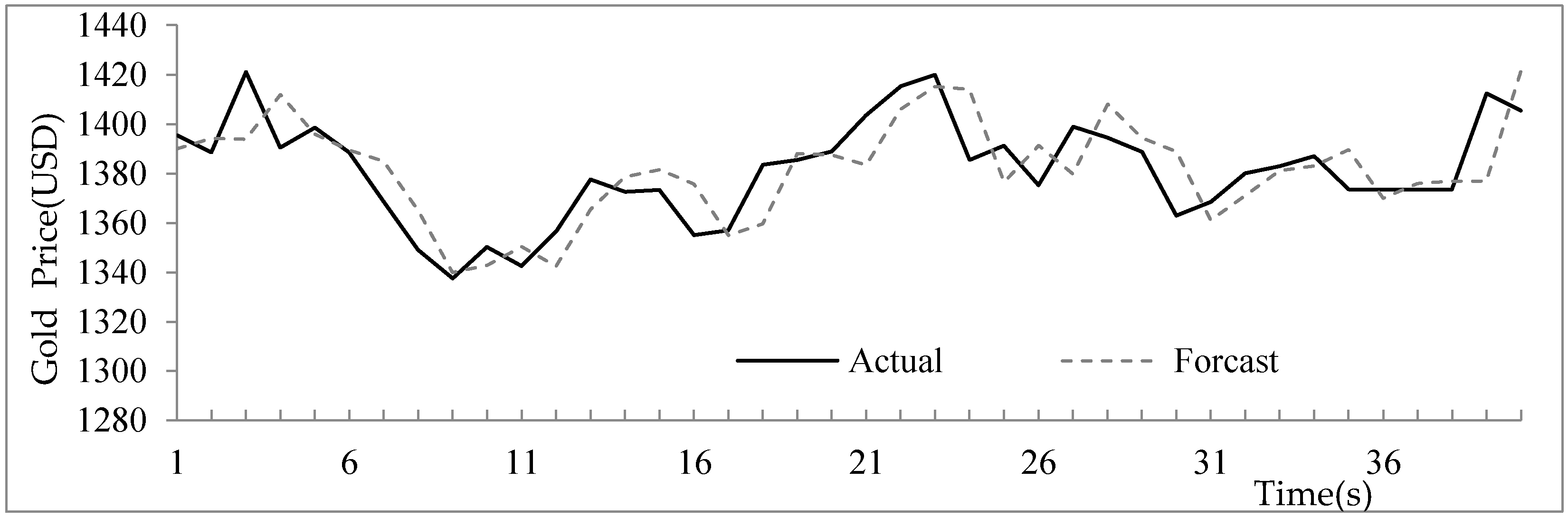
We also applied the proposed method to forecast the international gold price in USD from 2000 to 2010. We chose the COMEX gold price as a secondary factor. For each year, the authentic datasets of the historical daily closing prices from January to October were used as the training data, and the datasets from November to December were the testing data. The RMSEs of the forecast errors are shown in Table 8. Taking the 2010 gold price as an example, the forecast results are shown in Figure 3.
We can see that the proposed model can accurately forecast the international gold price.
5. Conclusions
In this paper, a new forecasting model is proposed based on a first-order two-factor ARMA(1,m) model. The proposed method is based on the fluctuations of two time series. The secondary factor was used to modify the forecast performance of the main factor. The experiments showed that the fuzzy logic relations of the main and secondary factors obtained from the two training datasets can successfully predict the testing dataset of the main factor. To compare the performance with other methods, we employed TAIEX 2004 as an example to illustrate our process. We also forecasted TAIEX 1997–2005, SHSECI 2001–2015, and the international gold price 2000–2010 to show its accuracy and versatility. For future research, we may consider additional aspects of the stock markets such as volumes, ending prices, opening prices, etc. A third factor, or more, could be used to modify the forecasting process.
Acknowledgments
The authors are indebted to anonymous reviewers for their very insightful comments and constructive suggestions, which help ameliorate the quality of this paper. This work supported by the National Research Foundation of Korea Grant funded by the Korean Government(NRF-2014S1A2A2027622) and the Foundation Program of Jiangsu University (16JDG005).
Author Contributions
Shuang Guan designed the experiments and wrote the paper; Aiwu Zhao conceived the main idea of the method.
Conflicts of Interest
The authors declare no conflict of interest.
Appendix A
The historical training dataset can be represented by a fuzzified fluctuation dataset as shown in Table A1 and Table A2.

Table A1.
Historical training data and fuzzified fluctuation data of TAIEX2004.
| Date (MM/DD/YYYY) | TAIEX | Fluctuation | Fuzzified | Date (MM/DD/YYYY) | TAIEX | Fluctuation | Fuzzified | Date (MM/DD/YYYY) | TAIEX | Fluctuation | Fuzzified |
|---|---|---|---|---|---|---|---|---|---|---|---|
| 01/02/2004 | 6041.56 | - | - | 04/16/2004 | 6818.20 | 81.41 | 5 | 07/23/2004 | 5373.85 | −14.11 | 3 |
| 01/05/2004 | 6125.42 | 83.86 | 5 | 04/19/2004 | 6779.18 | −39.02 | 2 | 07/26/2004 | 5331.71 | −42.14 | 2 |
| 01/06/2004 | 6144.01 | 18.59 | 4 | 04/20/2004 | 6799.97 | 20.79 | 4 | 07/27/2004 | 5398.61 | 66.90 | 5 |
| 01/07/2004 | 6141.25 | −2.76 | 3 | 04/21/2004 | 6810.25 | 10.28 | 3 | 07/28/2004 | 5383.57 | −15.04 | 3 |
| 01/08/2004 | 6169.17 | 27.92 | 4 | 04/22/2004 | 6732.09 | −78.16 | 1 | 07/29/2004 | 5349.66 | −33.91 | 2 |
| 01/09/2004 | 6226.98 | 57.81 | 5 | 04/23/2004 | 6748.10 | 16.01 | 3 | 07/30/2004 | 5420.57 | 70.91 | 5 |
| 01/12/2004 | 6219.71 | −7.27 | 3 | 04/26/2004 | 6710.70 | −37.40 | 2 | 08/02/2004 | 5350.40 | −70.17 | 1 |
| 01/13/2004 | 6210.22 | −9.49 | 3 | 04/27/2004 | 6646.80 | −63.90 | 1 | 08/03/2004 | 5367.22 | 16.82 | 4 |
| 01/14/2004 | 6274.97 | 64.75 | 5 | 04/28/2004 | 6574.75 | −72.05 | 1 | 08/04/2004 | 5316.87 | −50.35 | 1 |
| 01/15/2004 | 6264.37 | −10.60 | 3 | 04/29/2004 | 6402.21 | −172.54 | 1 | 08/05/2004 | 5427.61 | 110.74 | 5 |
| 01/16/2004 | 6269.71 | 5.34 | 3 | 04/30/2004 | 6117.81 | −284.40 | 1 | 08/06/2004 | 5399.16 | −28.45 | 2 |
| 01/27/2004 | 6384.63 | 114.92 | 5 | 05/03/2004 | 6029.77 | −88.04 | 1 | 08/09/2004 | 5399.45 | 0.29 | 3 |
| 01/28/2004 | 6386.25 | 1.62 | 3 | 05/04/2004 | 6188.15 | 158.38 | 5 | 08/10/2004 | 5393.73 | −5.72 | 3 |
| 01/29/2004 | 6312.65 | −73.60 | 1 | 05/05/2004 | 5854.23 | −333.92 | 1 | 08/11/2004 | 5367.34 | −26.39 | 2 |
| 01/30/2004 | 6375.38 | 62.73 | 5 | 05/06/2004 | 5909.79 | 55.56 | 5 | 08/12/2004 | 5368.02 | 0.68 | 3 |
| 02/02/2004 | 6319.96 | −55.42 | 1 | 05/07/2004 | 6040.26 | 130.47 | 5 | 08/13/2004 | 5389.93 | 21.91 | 4 |
| 02/03/2004 | 6252.23 | −67.73 | 1 | 05/10/2004 | 5825.05 | −215.21 | 1 | 08/16/2004 | 5352.01 | −37.92 | 2 |
| 02/04/2004 | 6241.39 | −10.84 | 3 | 05/11/2004 | 5886.36 | 61.31 | 5 | 08/17/2004 | 5342.49 | −9.52 | 3 |
| 02/05/2004 | 6268.14 | 26.75 | 4 | 05/12/2004 | 5958.79 | 72.43 | 5 | 08/18/2004 | 5427.75 | 85.26 | 5 |
| 02/06/2004 | 6353.35 | 85.21 | 5 | 05/13/2004 | 5918.09 | −40.70 | 2 | 08/19/2004 | 5602.99 | 175.24 | 5 |
| 02/09/2004 | 6463.09 | 109.74 | 5 | 05/14/2004 | 5777.32 | −140.77 | 1 | 08/20/2004 | 5622.86 | 19.87 | 4 |
| 02/10/2004 | 6488.34 | 25.25 | 4 | 05/17/2004 | 5482.96 | −294.36 | 1 | 08/23/2004 | 5660.97 | 38.11 | 4 |
| 02/11/2004 | 6454.39 | −33.95 | 2 | 05/18/2004 | 5557.68 | 74.72 | 5 | 08/26/2004 | 5813.39 | 152.42 | 5 |
| 02/12/2004 | 6436.95 | −17.44 | 2 | 05/19/2004 | 5860.58 | 302.90 | 5 | 08/27/2004 | 5797.71 | −15.68 | 3 |
| 02/13/2004 | 6549.18 | 112.23 | 5 | 05/20/2004 | 5815.33 | −45.25 | 2 | 08/30/2004 | 5788.94 | −8.77 | 3 |
| 02/16/2004 | 6565.37 | 16.19 | 3 | 05/21/2004 | 5964.94 | 149.61 | 5 | 08/31/2004 | 5765.54 | −23.40 | 2 |
| 02/17/2004 | 6600.47 | 35.10 | 4 | 05/24/2004 | 5942.08 | −22.86 | 2 | 09/01/2004 | 5858.14 | 92.60 | 5 |
| 02/18/2004 | 6605.85 | 5.38 | 3 | 05/25/2004 | 5958.38 | 16.30 | 3 | 09/02/2004 | 5852.85 | −5.29 | 3 |
| 02/19/2004 | 6681.52 | 75.67 | 5 | 05/26/2004 | 6027.27 | 68.89 | 5 | 09/03/2004 | 5761.14 | −91.71 | 1 |
| 02/20/2004 | 6665.54 | −15.98 | 3 | 05/27/2004 | 6033.05 | 5.78 | 3 | 09/06/2004 | 5775.99 | 14.85 | 3 |
| 02/23/2004 | 6665.89 | 0.35 | 3 | 05/28/2004 | 6137.26 | 104.21 | 5 | 09/07/2004 | 5846.83 | 70.84 | 5 |
| 02/24/2004 | 6589.23 | −76.66 | 1 | 05/31/2004 | 5977.84 | −159.42 | 1 | 09/08/2004 | 5846.02 | −0.81 | 3 |
| 02/25/2004 | 6644.28 | 55.05 | 5 | 06/01/2004 | 5986.20 | 8.36 | 3 | 09/09/2004 | 5842.93 | −3.09 | 3 |
| 02/26/2004 | 6693.25 | 48.97 | 4 | 06/02/2004 | 5875.67 | −110.53 | 1 | 09/10/2004 | 5846.19 | 3.26 | 3 |
| 02/27/2004 | 6750.54 | 57.29 | 5 | 06/03/2004 | 5671.45 | −204.22 | 1 | 09/13/2004 | 5928.22 | 82.03 | 5 |
| 03/01/2004 | 6888.43 | 137.89 | 5 | 06/04/2004 | 5724.89 | 53.44 | 5 | 09/14/2004 | 5919.77 | −8.45 | 3 |
| 03/02/2004 | 6975.26 | 86.83 | 5 | 06/07/2004 | 5935.82 | 210.93 | 5 | 09/15/2004 | 5871.07 | −48.70 | 2 |
| 03/03/2004 | 6932.17 | −43.09 | 2 | 06/08/2004 | 5986.76 | 50.94 | 5 | 09/16/2004 | 5891.05 | 19.98 | 4 |
| 03/04/2004 | 7034.10 | 101.93 | 5 | 06/09/2004 | 5965.70 | −21.06 | 2 | 09/17/2004 | 5818.39 | −72.66 | 1 |
| 03/05/2004 | 6943.68 | −90.42 | 1 | 06/10/2004 | 5867.51 | −98.19 | 1 | 09/20/2004 | 5864.54 | 46.15 | 4 |
| 03/08/2004 | 6901.48 | −42.20 | 2 | 06/11/2004 | 5735.07 | −132.44 | 1 | 09/21/2004 | 5949.26 | 84.72 | 5 |
| 03/09/2004 | 6973.90 | 72.42 | 5 | 06/14/2004 | 5574.08 | −160.99 | 1 | 09/22/2004 | 5970.18 | 20.92 | 4 |
| 03/10/2004 | 6874.91 | −98.99 | 1 | 06/15/2004 | 5646.49 | 72.41 | 5 | 09/23/2004 | 5937.25 | −32.93 | 2 |
| 03/11/2004 | 6879.11 | 4.20 | 3 | 06/16/2004 | 5560.16 | −86.33 | 1 | 09/24/2004 | 5892.21 | −45.04 | 2 |
| 03/12/2004 | 6800.24 | −78.87 | 1 | 06/17/2004 | 5664.35 | 104.19 | 5 | 09/27/2004 | 5849.22 | −42.99 | 2 |
| 03/15/2004 | 6635.98 | −164.26 | 1 | 06/18/2004 | 5569.29 | −95.06 | 1 | 09/29/2004 | 5809.75 | −39.47 | 2 |
| 03/16/2004 | 6589.72 | −46.26 | 2 | 06/21/2004 | 5556.54 | −12.75 | 3 | 09/30/2004 | 5845.69 | 35.94 | 4 |
| 03/17/2004 | 6577.98 | −11.74 | 3 | 06/23/2004 | 5729.30 | 172.76 | 5 | 10/01/2004 | 5945.35 | 99.66 | 5 |
| 03/18/2004 | 6787.03 | 209.05 | 5 | 06/24/2004 | 5779.09 | 49.79 | 4 | 10/04/2004 | 6077.96 | 132.61 | 5 |
| 03/19/2004 | 6815.09 | 28.06 | 4 | 06/25/2004 | 5802.55 | 23.46 | 4 | 10/05/2004 | 6081.01 | 3.05 | 3 |
| 03/22/2004 | 6359.92 | −455.17 | 1 | 06/28/2004 | 5709.84 | −92.71 | 1 | 10/06/2004 | 6060.61 | −20.40 | 2 |
| 03/23/2004 | 6172.89 | −187.03 | 1 | 06/29/2004 | 5741.52 | 31.68 | 4 | 10/07/2004 | 6103.00 | 42.39 | 4 |
| 03/24/2004 | 6213.56 | 40.67 | 4 | 06/30/2004 | 5839.44 | 97.92 | 5 | 10/08/2004 | 6102.16 | −0.84 | 3 |
| 03/25/2004 | 6156.73 | −56.83 | 1 | 07/01/2004 | 5836.91 | −2.53 | 3 | 10/11/2004 | 6089.28 | −12.88 | 3 |
| 03/26/2004 | 6132.62 | −24.11 | 2 | 07/02/2004 | 5746.70 | −90.21 | 1 | 10/12/2004 | 5979.56 | −109.72 | 1 |
| 03/29/2004 | 6474.11 | 341.49 | 5 | 07/05/2004 | 5659.78 | −86.92 | 1 | 10/13/2004 | 5963.07 | −16.49 | 3 |
| 03/30/2004 | 6494.71 | 20.60 | 4 | 07/06/2004 | 5733.57 | 73.79 | 5 | 10/14/2004 | 5831.07 | −132.00 | 1 |
| 03/31/2004 | 6522.19 | 27.48 | 4 | 07/07/2004 | 5727.78 | −5.79 | 3 | 10/15/2004 | 5820.82 | −10.25 | 3 |
| 04/01/2004 | 6523.49 | 1.30 | 3 | 07/08/2004 | 5713.39 | −14.39 | 3 | 10/18/2004 | 5772.12 | −48.70 | 2 |
| 04/02/2004 | 6545.54 | 22.05 | 4 | 07/09/2004 | 5777.72 | 64.33 | 5 | 10/19/2004 | 5807.79 | 35.67 | 4 |
| 04/05/2004 | 6682.73 | 137.19 | 5 | 07/12/2004 | 5758.74 | −18.98 | 2 | 10/20/2004 | 5788.34 | −19.45 | 2 |
| 04/06/2004 | 6635.54 | −47.19 | 2 | 07/13/2004 | 5685.57 | −73.17 | 1 | 10/21/2004 | 5797.24 | 8.90 | 3 |
| 04/07/2004 | 6646.74 | 11.20 | 3 | 07/14/2004 | 5623.65 | −61.92 | 1 | 10/22/2004 | 5774.67 | −22.57 | 2 |
| 04/08/2004 | 6672.86 | 26.12 | 4 | 07/15/2004 | 5542.80 | −80.85 | 1 | 10/26/2004 | 5662.88 | −111.79 | 1 |
| 04/09/2004 | 6620.36 | −52.50 | 1 | 07/16/2004 | 5502.14 | −40.66 | 2 | 10/27/2004 | 5650.97 | −11.91 | 3 |
| 04/12/2004 | 6777.78 | 157.42 | 5 | 07/19/2004 | 5489.10 | −13.04 | 3 | 10/28/2004 | 5695.56 | 44.59 | 4 |
| 04/13/2004 | 6794.33 | 16.55 | 3 | 07/20/2004 | 5325.68 | −163.42 | 1 | 10/29/2004 | 5705.93 | 10.37 | 3 |
| 04/14/2004 | 6880.18 | 85.85 | 5 | 07/21/2004 | 5409.13 | 83.45 | 5 | ||||
| 04/15/2004 | 6736.79 | −143.39 | 1 | 07/22/2004 | 5387.96 | −21.17 | 2 |
Table A2.
Historical training data and fuzzified fluctuation data of Dow Jones 2004.
| Date (MM/DD/YYYY) | TAIEX | Fluctuation | Fuzzified | Date (MM/DD/YYYY) | TAIEX | Fluctuation | Fuzzified | Date (MM/DD/YYYY) | TAIEX | Fluctuation | Fuzzified |
|---|---|---|---|---|---|---|---|---|---|---|---|
| 01/02/2004 | 10409.85 | - | - | 04/14/2004 | 10377.95 | −3.33 | 3 | 07/26/2004 | 9961.92 | −0.30 | 3 |
| 01/05/2004 | 10544.07 | 134.22 | 5 | 04/15/2004 | 10397.46 | 19.51 | 4 | 07/27/2004 | 10085.14 | 123.22 | 5 |
| 01/06/2004 | 10538.66 | −5.41 | 3 | 04/16/2004 | 10451.97 | 54.51 | 5 | 07/28/2004 | 10117.07 | 31.93 | 4 |
| 01/07/2004 | 10529.03 | −9.63 | 3 | 04/19/2004 | 10437.85 | −14.12 | 2 | 07/29/2004 | 10129.24 | 12.17 | 3 |
| 01/08/2004 | 10592.44 | 63.41 | 5 | 04/20/2004 | 10314.50 | −123.35 | 1 | 07/30/2004 | 10139.71 | 10.47 | 3 |
| 01/09/2004 | 10458.89 | −133.55 | 1 | 04/21/2004 | 10317.27 | 2.77 | 3 | 08/02/2004 | 10179.16 | 39.45 | 4 |
| 01/12/2004 | 10485.18 | 26.29 | 4 | 04/22/2004 | 10461.20 | 143.93 | 5 | 08/03/2004 | 10120.24 | −58.92 | 1 |
| 01/13/2004 | 10427.18 | −58.00 | 1 | 04/23/2004 | 10472.84 | 11.64 | 3 | 08/04/2004 | 10126.51 | 6.27 | 3 |
| 01/14/2004 | 10538.37 | 111.19 | 5 | 04/26/2004 | 10444.73 | −28.11 | 2 | 08/05/2004 | 9963.03 | −163.48 | 1 |
| 01/15/2004 | 10553.85 | 15.48 | 4 | 04/27/2004 | 10478.16 | 33.43 | 4 | 08/06/2004 | 9815.33 | −147.70 | 1 |
| 01/16/2004 | 10600.51 | 46.66 | 5 | 04/28/2004 | 10342.60 | −135.56 | 1 | 08/09/2004 | 9814.66 | −0.67 | 3 |
| 01/20/2004 | 10528.66 | −71.85 | 1 | 04/29/2004 | 10272.27 | −70.33 | 1 | 08/10/2004 | 9944.67 | 130.01 | 5 |
| 01/21/2004 | 10623.62 | 94.96 | 5 | 04/30/2004 | 10225.57 | −46.70 | 1 | 08/11/2004 | 9938.32 | −6.35 | 3 |
| 01/22/2004 | 10623.18 | −0.44 | 3 | 05/03/2004 | 10314.00 | 88.43 | 5 | 08/12/2004 | 9814.59 | −123.73 | 1 |
| 01/23/2004 | 10568.29 | −54.89 | 1 | 05/04/2004 | 10317.20 | 3.20 | 3 | 08/13/2004 | 9825.35 | 10.76 | 3 |
| 01/26/2004 | 10702.51 | 134.22 | 5 | 05/05/2004 | 10310.95 | −6.25 | 3 | 08/16/2004 | 9954.55 | 129.20 | 5 |
| 01/27/2004 | 10609.92 | −92.59 | 1 | 05/06/2004 | 10241.26 | −69.69 | 1 | 08/17/2004 | 9972.83 | 18.28 | 4 |
| 01/28/2004 | 10468.37 | −141.55 | 1 | 05/07/2004 | 10117.34 | −123.92 | 1 | 08/18/2004 | 10083.15 | 110.32 | 5 |
| 01/29/2004 | 10510.29 | 41.92 | 5 | 05/10/2004 | 9990.02 | −127.32 | 1 | 08/19/2004 | 10040.82 | −42.33 | 1 |
| 01/30/2004 | 10488.07 | −22.22 | 2 | 05/11/2004 | 10019.47 | 29.45 | 4 | 08/20/2004 | 10110.14 | 69.32 | 5 |
| 02/02/2004 | 10499.18 | 11.11 | 3 | 05/12/2004 | 10045.16 | 25.69 | 4 | 08/23/2004 | 10073.05 | −37.09 | 2 |
| 02/03/2004 | 10505.18 | 6.00 | 3 | 05/13/2004 | 10010.74 | −34.42 | 2 | 08/24/2004 | 10098.63 | 25.58 | 4 |
| 02/04/2004 | 10470.74 | −34.44 | 2 | 05/14/2004 | 10012.87 | 2.13 | 3 | 08/25/2004 | 10181.74 | 83.11 | 5 |
| 02/05/2004 | 10495.55 | 24.81 | 4 | 05/17/2004 | 9906.91 | −105.96 | 1 | 08/26/2004 | 10173.41 | −8.33 | 3 |
| 02/06/2004 | 10593.03 | 97.48 | 5 | 05/18/2004 | 9968.51 | 61.60 | 5 | 08/27/2004 | 10195.01 | 21.60 | 4 |
| 02/09/2004 | 10579.03 | −14.00 | 2 | 05/19/2004 | 9937.71 | −30.80 | 2 | 08/30/2004 | 10122.52 | −72.49 | 1 |
| 02/10/2004 | 10613.85 | 34.82 | 4 | 05/20/2004 | 9937.64 | −0.07 | 3 | 08/31/2004 | 10173.92 | 51.40 | 5 |
| 02/11/2004 | 10737.70 | 123.85 | 5 | 05/21/2004 | 9966.74 | 29.10 | 4 | 09/01/2004 | 10168.46 | −5.46 | 3 |
| 02/12/2004 | 10694.07 | −43.63 | 1 | 05/24/2004 | 9958.43 | −8.31 | 3 | 09/02/2004 | 10290.28 | 121.82 | 5 |
| 02/13/2004 | 10627.85 | −66.22 | 1 | 05/25/2004 | 10117.62 | 159.19 | 5 | 09/03/2004 | 10260.20 | −30.08 | 2 |
| 02/17/2004 | 10714.88 | 87.03 | 5 | 05/26/2004 | 10109.89 | −7.73 | 3 | 09/07/2004 | 10341.16 | 80.96 | 5 |
| 02/18/2004 | 10671.99 | −42.89 | 1 | 05/27/2004 | 10205.20 | 95.31 | 5 | 09/08/2004 | 10313.36 | −27.80 | 2 |
| 02/19/2004 | 10664.73 | −7.26 | 3 | 05/28/2004 | 10188.45 | −16.75 | 2 | 09/09/2004 | 10289.10 | −24.26 | 2 |
| 02/20/2004 | 10619.03 | −45.70 | 1 | 06/01/2004 | 10202.65 | 14.20 | 4 | 09/10/2004 | 10313.07 | 23.97 | 4 |
| 02/23/2004 | 10609.62 | −9.41 | 3 | 06/02/2004 | 10262.97 | 60.32 | 5 | 09/13/2004 | 10314.76 | 1.69 | 3 |
| 02/24/2004 | 10566.37 | −43.25 | 1 | 06/03/2004 | 10195.91 | −67.06 | 1 | 09/14/2004 | 10318.16 | 3.40 | 3 |
| 02/25/2004 | 10601.62 | 35.25 | 4 | 06/04/2004 | 10242.82 | 46.91 | 5 | 09/15/2004 | 10231.36 | −86.80 | 1 |
| 02/26/2004 | 10580.14 | −21.48 | 2 | 06/07/2004 | 10391.08 | 148.26 | 5 | 09/16/2004 | 10244.49 | 13.13 | 3 |
| 02/27/2004 | 10583.92 | 3.78 | 3 | 06/08/2004 | 10432.52 | 41.44 | 5 | 09/17/2004 | 10284.46 | 39.97 | 4 |
| 03/01/2004 | 10678.14 | 94.22 | 5 | 06/09/2004 | 10368.44 | −64.08 | 1 | 09/20/2004 | 10204.89 | −79.57 | 1 |
| 03/02/2004 | 10591.48 | −86.66 | 1 | 06/10/2004 | 10410.10 | 41.66 | 5 | 09/21/2004 | 10244.93 | 40.04 | 4 |
| 03/03/2004 | 10593.11 | 1.63 | 3 | 06/14/2004 | 10334.73 | −75.37 | 1 | 09/22/2004 | 10109.18 | −135.75 | 1 |
| 03/04/2004 | 10588.00 | −5.11 | 3 | 06/15/2004 | 10380.43 | 45.70 | 5 | 09/23/2004 | 10038.90 | −70.28 | 1 |
| 03/05/2004 | 10595.55 | 7.55 | 3 | 06/16/2004 | 10379.58 | −0.85 | 3 | 09/24/2004 | 10047.24 | 8.34 | 3 |
| 03/08/2004 | 10529.48 | −66.07 | 1 | 06/17/2004 | 10377.52 | −2.06 | 3 | 09/27/2004 | 9988.54 | −58.70 | 1 |
| 03/09/2004 | 10456.96 | −72.52 | 1 | 06/18/2004 | 10416.41 | 38.89 | 4 | 09/28/2004 | 10077.40 | 88.86 | 5 |
| 03/10/2004 | 10296.89 | −160.07 | 1 | 06/21/2004 | 10371.47 | −44.94 | 1 | 09/29/2004 | 10136.24 | 58.84 | 5 |
| 03/11/2004 | 10128.38 | −168.51 | 1 | 06/22/2004 | 10395.07 | 23.60 | 4 | 09/30/2004 | 10080.27 | −55.97 | 1 |
| 03/12/2004 | 10240.08 | 111.70 | 5 | 06/23/2004 | 10479.57 | 84.50 | 5 | 10/01/2004 | 10192.65 | 112.38 | 5 |
| 03/15/2004 | 10102.89 | −137.19 | 1 | 06/24/2004 | 10443.81 | −35.76 | 2 | 10/04/2004 | 10216.54 | 23.89 | 4 |
| 03/16/2004 | 10184.67 | 81.78 | 5 | 06/25/2004 | 10371.84 | −71.97 | 1 | 10/05/2004 | 10177.68 | −38.86 | 2 |
| 03/17/2004 | 10300.30 | 115.63 | 5 | 06/28/2004 | 10357.09 | −14.75 | 2 | 10/06/2004 | 10239.92 | 62.24 | 5 |
| 03/18/2004 | 10295.78 | −4.52 | 3 | 06/29/2004 | 10413.43 | 56.34 | 5 | 10/07/2004 | 10125.40 | −114.52 | 1 |
| 03/19/2004 | 10186.60 | −109.18 | 1 | 06/30/2004 | 10435.48 | 22.05 | 4 | 10/08/2004 | 10055.20 | −70.20 | 1 |
| 03/22/2004 | 10064.75 | −121.85 | 1 | 07/01/2004 | 10334.16 | −101.32 | 1 | 10/11/2004 | 10081.97 | 26.77 | 4 |
| 03/23/2004 | 10063.64 | −1.11 | 3 | 07/02/2004 | 10282.83 | −51.33 | 1 | 10/12/2004 | 10077.18 | −4.79 | 3 |
| 03/24/2004 | 10048.23 | −15.41 | 2 | 07/06/2004 | 10219.34 | −63.49 | 1 | 10/13/2004 | 10002.33 | −74.85 | 1 |
| 03/25/2004 | 10218.82 | 170.59 | 5 | 07/07/2004 | 10240.29 | 20.95 | 4 | 10/14/2004 | 9894.45 | −107.88 | 1 |
| 03/26/2004 | 10212.97 | −5.85 | 3 | 07/08/2004 | 10171.56 | −68.73 | 1 | 10/15/2004 | 9933.38 | 38.93 | 4 |
| 03/29/2004 | 10329.63 | 116.66 | 5 | 07/09/2004 | 10213.22 | 41.66 | 5 | 10/18/2004 | 9956.32 | 22.94 | 4 |
| 03/30/2004 | 10381.70 | 52.07 | 5 | 07/12/2004 | 10238.22 | 25.00 | 4 | 10/19/2004 | 9897.62 | −58.70 | 1 |
| 03/31/2004 | 10357.70 | −24.00 | 2 | 07/13/2004 | 10247.59 | 9.37 | 3 | 10/20/2004 | 9886.93 | −10.69 | 3 |
| 04/01/2004 | 10373.33 | 15.63 | 4 | 07/14/2004 | 10208.80 | −38.79 | 2 | 10/21/2004 | 9865.76 | −21.17 | 2 |
| 04/02/2004 | 10470.59 | 97.26 | 5 | 07/15/2004 | 10163.16 | −45.64 | 1 | 10/22/2004 | 9757.81 | −107.95 | 1 |
| 04/05/2004 | 10558.37 | 87.78 | 5 | 07/16/2004 | 10139.78 | −23.38 | 2 | 10/25/2004 | 9749.99 | −7.82 | 3 |
| 04/06/2004 | 10570.81 | 12.44 | 3 | 07/19/2004 | 10094.06 | −45.72 | 1 | 10/26/2004 | 9888.48 | 138.49 | 5 |
| 04/07/2004 | 10480.15 | −90.66 | 1 | 07/20/2004 | 10149.07 | 55.01 | 5 | 10/27/2004 | 10002.03 | 113.55 | 5 |
| 04/08/2004 | 10442.03 | −38.12 | 2 | 07/21/2004 | 10046.13 | −102.94 | 1 | 10/28/2004 | 10004.54 | 2.51 | 3 |
| 04/12/2004 | 10515.56 | 73.53 | 5 | 07/22/2004 | 10050.33 | 4.20 | 3 | 10/29/2004 | 10027.47 | 22.93 | 4 |
| 04/13/2004 | 10381.28 | −134.28 | 1 | 07/23/2004 | 9962.22 | −88.11 | 1 |
Appendix B
The fluctuation error series of training data is shown in Table A3.
Table A3.
The Fluctuation Error Series.
| Date | TAIEX Group | Dow Jones Group | Actual | Forecast | Fluctuation | Fuzzified | Date | TAIEX Group | Dow Jones Group | Actual | Forecast | Fluctuation | Fuzzified |
|---|---|---|---|---|---|---|---|---|---|---|---|---|---|
| TAIEX | TAIEX | Group of Fluctuation | TAIEX | TAIEX | Group of Fluctuation | ||||||||
| 01/05/2004 | 3 | 3 | 6125.42 | 6041.56 | 83.86 | 5 | 06/03/2004 | 1 | 5 | 5671.45 | 5871.95 | −200.50 | 1 |
| 01/06/2004 | 5 | 5 | 6144.01 | 6144.81 | −0.80 | 3 | 06/04/2004 | 1 | 1 | 5724.89 | 5671.45 | 53.44 | 5 |
| 01/07/2004 | 4 | 3 | 6141.25 | 6118.88 | 22.37 | 4 | 06/07/2004 | 5 | 5 | 5935.82 | 5744.28 | 191.54 | 5 |
| 01/08/2004 | 3 | 3 | 6169.17 | 6141.25 | 27.92 | 4 | 06/08/2004 | 5 | 5 | 5986.76 | 5955.21 | 31.55 | 4 |
| 01/09/2004 | 4 | 5 | 6226.98 | 6213.84 | 13.14 | 3 | 06/09/2004 | 5 | 5 | 5965.70 | 6006.15 | −40.45 | 2 |
| 01/12/2004 | 5 | 1 | 6219.71 | 6214.80 | 4.91 | 3 | 06/10/2004 | 2 | 1 | 5867.51 | 5961.51 | −94.00 | 1 |
| 01/13/2004 | 3 | 4 | 6210.22 | 6216.66 | −6.44 | 3 | 06/11/2004 | 1 | 5 | 5735.07 | 5863.79 | −128.72 | 1 |
| 01/14/2004 | 3 | 1 | 6274.97 | 6210.22 | 64.75 | 5 | 06/14/2004 | 1 | 1 | 5574.08 | 5735.07 | −160.99 | 1 |
| 01/15/2004 | 5 | 5 | 6264.37 | 6294.36 | −29.99 | 2 | 06/15/2004 | 1 | 1 | 5646.49 | 5574.08 | 72.41 | 5 |
| 01/16/2004 | 3 | 4 | 6269.71 | 6261.32 | 8.39 | 3 | 06/16/2004 | 5 | 5 | 5560.16 | 5665.88 | −105.72 | 1 |
| 01/27/2004 | 3 | 5 | 6384.63 | 6298.42 | 86.21 | 5 | 06/17/2004 | 1 | 3 | 5664.35 | 5560.16 | 104.19 | 5 |
| 01/28/2004 | 5 | 1 | 6386.25 | 6372.45 | 13.80 | 3 | 06/18/2004 | 5 | 3 | 5569.29 | 5644.81 | −75.52 | 1 |
| 01/29/2004 | 3 | 1 | 6312.65 | 6386.25 | −73.60 | 1 | 06/21/2004 | 1 | 4 | 5556.54 | 5582.69 | −26.15 | 2 |
| 01/30/2004 | 1 | 5 | 6375.38 | 6308.93 | 66.45 | 5 | 06/23/2004 | 3 | 1 | 5729.30 | 5556.54 | 172.76 | 5 |
| 02/02/2004 | 5 | 2 | 6319.96 | 6341.88 | −21.92 | 2 | 06/24/2004 | 5 | 5 | 5779.09 | 5748.69 | 30.40 | 4 |
| 02/03/2004 | 1 | 3 | 6252.23 | 6319.96 | −67.73 | 1 | 06/25/2004 | 4 | 2 | 5802.55 | 5784.67 | 17.88 | 4 |
| 02/04/2004 | 1 | 3 | 6241.39 | 6252.23 | −10.84 | 3 | 06/28/2004 | 4 | 1 | 5709.84 | 5787.66 | −77.82 | 1 |
| 02/05/2004 | 3 | 2 | 6268.14 | 6234.69 | 33.45 | 4 | 06/29/2004 | 1 | 2 | 5741.52 | 5698.67 | 42.85 | 4 |
| 02/06/2004 | 4 | 4 | 6353.35 | 6284.89 | 68.46 | 5 | 06/30/2004 | 4 | 5 | 5839.44 | 5786.19 | 53.25 | 5 |
| 02/09/2004 | 5 | 5 | 6463.09 | 6372.74 | 90.35 | 5 | 07/01/2004 | 5 | 4 | 5836.91 | 5849.01 | −12.10 | 3 |
| 02/10/2004 | 5 | 2 | 6488.34 | 6429.59 | 58.75 | 5 | 07/02/2004 | 3 | 1 | 5746.70 | 5836.91 | −90.21 | 1 |
| 02/11/2004 | 4 | 4 | 6454.39 | 6505.09 | −50.70 | 1 | 07/05/2004 | 1 | 1 | 5659.78 | 5746.70 | −86.92 | 1 |
| 02/12/2004 | 2 | 5 | 6436.95 | 6471.14 | −34.19 | 2 | 07/06/2004 | 1 | 1 | 5733.57 | 5659.78 | 73.79 | 5 |
| 02/13/2004 | 2 | 1 | 6549.18 | 6432.76 | 116.42 | 5 | 07/07/2004 | 5 | 1 | 5727.78 | 5721.39 | 6.39 | 3 |
| 02/16/2004 | 5 | 1 | 6565.37 | 6537.00 | 28.37 | 4 | 07/08/2004 | 3 | 4 | 5713.39 | 5724.73 | −11.34 | 3 |
| 02/17/2004 | 3 | 3 | 6600.47 | 6565.37 | 35.10 | 4 | 07/09/2004 | 3 | 1 | 5777.72 | 5713.39 | 64.33 | 5 |
| 02/18/2004 | 4 | 5 | 6605.85 | 6645.14 | −39.29 | 2 | 07/12/2004 | 5 | 5 | 5758.74 | 5797.11 | −38.37 | 2 |
| 02/19/2004 | 3 | 1 | 6681.52 | 6605.85 | 75.67 | 5 | 07/13/2004 | 2 | 4 | 5685.57 | 5741.99 | −56.42 | 1 |
| 02/20/2004 | 5 | 3 | 6665.54 | 6661.98 | 3.56 | 3 | 07/14/2004 | 1 | 3 | 5623.65 | 5685.57 | −61.92 | 1 |
| 02/23/2004 | 3 | 1 | 6665.89 | 6665.54 | 0.35 | 3 | 07/15/2004 | 1 | 2 | 5542.80 | 5612.48 | −69.68 | 1 |
| 02/24/2004 | 3 | 3 | 6589.23 | 6665.89 | −76.66 | 1 | 07/16/2004 | 1 | 1 | 5502.14 | 5542.80 | −40.66 | 2 |
| 02/25/2004 | 1 | 1 | 6644.28 | 6589.23 | 55.05 | 5 | 07/19/2004 | 2 | 2 | 5489.10 | 5477.01 | 12.09 | 3 |
| 02/26/2004 | 5 | 4 | 6693.25 | 6653.85 | 39.40 | 4 | 07/20/2004 | 3 | 1 | 5325.68 | 5489.10 | −163.42 | 1 |
| 02/27/2004 | 4 | 2 | 6750.54 | 6698.83 | 51.71 | 5 | 07/21/2004 | 1 | 5 | 5409.13 | 5321.96 | 87.17 | 5 |
| 03/01/2004 | 5 | 3 | 6888.43 | 6731.00 | 157.43 | 5 | 07/22/2004 | 5 | 1 | 5387.96 | 5396.95 | −8.99 | 3 |
| 03/02/2004 | 5 | 5 | 6975.26 | 6907.82 | 67.44 | 5 | 07/23/2004 | 2 | 3 | 5373.85 | 5415.37 | −41.52 | 2 |
| 03/03/2004 | 5 | 1 | 6932.17 | 6963.08 | −30.91 | 2 | 07/26/2004 | 3 | 1 | 5331.71 | 5373.85 | −42.14 | 2 |
| 03/04/2004 | 2 | 3 | 7034.10 | 6959.58 | 74.52 | 5 | 07/27/2004 | 2 | 3 | 5398.61 | 5359.12 | 39.49 | 4 |
| 03/05/2004 | 5 | 3 | 6943.68 | 7014.56 | −70.88 | 1 | 07/28/2004 | 5 | 5 | 5383.57 | 5418.00 | −34.43 | 2 |
| 03/08/2004 | 1 | 3 | 6901.48 | 6943.68 | −42.20 | 2 | 07/29/2004 | 3 | 4 | 5349.66 | 5380.52 | −30.86 | 2 |
| 03/09/2004 | 2 | 1 | 6973.90 | 6897.29 | 76.61 | 5 | 07/30/2004 | 2 | 3 | 5420.57 | 5377.07 | 43.50 | 4 |
| 03/10/2004 | 5 | 1 | 6874.91 | 6961.72 | −86.81 | 1 | 08/02/2004 | 5 | 3 | 5350.40 | 5401.03 | −50.63 | 1 |
| 03/11/2004 | 1 | 1 | 6879.11 | 6874.91 | 4.20 | 3 | 08/03/2004 | 1 | 4 | 5367.22 | 5363.80 | 3.42 | 3 |
| 03/12/2004 | 3 | 1 | 6800.24 | 6879.11 | −78.87 | 1 | 08/04/2004 | 4 | 1 | 5316.87 | 5352.33 | −35.46 | 2 |
| 03/15/2004 | 1 | 5 | 6635.98 | 6796.52 | −160.54 | 1 | 08/05/2004 | 1 | 3 | 5427.61 | 5316.87 | 110.74 | 5 |
| 03/16/2004 | 1 | 1 | 6589.72 | 6635.98 | −46.26 | 2 | 08/06/2004 | 5 | 1 | 5399.16 | 5415.43 | −16.27 | 2 |
| 03/17/2004 | 2 | 5 | 6577.98 | 6606.47 | −28.49 | 2 | 08/09/2004 | 2 | 1 | 5399.45 | 5394.97 | 4.48 | 3 |
| 03/18/2004 | 3 | 5 | 6787.03 | 6606.69 | 180.34 | 5 | 08/10/2004 | 3 | 3 | 5393.73 | 5399.45 | −5.72 | 3 |
| 03/19/2004 | 5 | 3 | 6815.09 | 6767.49 | 47.60 | 4 | 08/11/2004 | 3 | 5 | 5367.34 | 5422.44 | −55.10 | 1 |
| 03/22/2004 | 4 | 1 | 6359.92 | 6800.20 | −440.28 | 1 | 08/12/2004 | 2 | 3 | 5368.02 | 5394.75 | −26.73 | 2 |
| 03/23/2004 | 1 | 1 | 6172.89 | 6359.92 | −187.03 | 1 | 08/13/2004 | 3 | 1 | 5389.93 | 5368.02 | 21.91 | 4 |
| 03/24/2004 | 1 | 3 | 6213.56 | 6172.89 | 40.67 | 4 | 08/16/2004 | 4 | 3 | 5352.01 | 5364.80 | −12.79 | 3 |
| 03/25/2004 | 4 | 2 | 6156.73 | 6219.14 | −62.41 | 1 | 08/17/2004 | 2 | 5 | 5342.49 | 5368.76 | −26.27 | 2 |
| 03/26/2004 | 1 | 5 | 6132.62 | 6153.01 | −20.39 | 2 | 08/18/2004 | 3 | 4 | 5427.75 | 5339.44 | 88.31 | 5 |
| 03/29/2004 | 2 | 3 | 6474.11 | 6160.03 | 314.08 | 5 | 08/19/2004 | 5 | 5 | 5602.99 | 5447.14 | 155.85 | 5 |
| 03/30/2004 | 5 | 5 | 6494.71 | 6493.50 | 1.21 | 3 | 08/20/2004 | 5 | 1 | 5622.86 | 5590.81 | 32.05 | 4 |
| 03/31/2004 | 4 | 5 | 6522.19 | 6539.38 | −17.19 | 2 | 08/23/2004 | 4 | 5 | 5660.97 | 5667.53 | −6.56 | 3 |
| 04/01/2004 | 4 | 2 | 6523.49 | 6527.77 | −4.28 | 3 | 08/26/2004 | 4 | 2 | 5813.39 | 5666.55 | 146.84 | 5 |
| 04/02/2004 | 3 | 4 | 6545.54 | 6520.44 | 25.10 | 4 | 08/27/2004 | 5 | 3 | 5797.71 | 5793.85 | 3.86 | 3 |
| 04/05/2004 | 4 | 5 | 6682.73 | 6590.21 | 92.52 | 5 | 08/30/2004 | 3 | 4 | 5788.94 | 5794.66 | −5.72 | 3 |
| 04/06/2004 | 5 | 5 | 6635.54 | 6702.12 | −66.58 | 1 | 08/31/2004 | 3 | 1 | 5765.54 | 5788.94 | −23.40 | 2 |
| 04/07/2004 | 2 | 3 | 6646.74 | 6662.95 | −16.21 | 2 | 09/01/2004 | 2 | 5 | 5858.14 | 5782.29 | 75.85 | 5 |
| 04/08/2004 | 3 | 1 | 6672.86 | 6646.74 | 26.12 | 4 | 09/02/2004 | 5 | 3 | 5852.85 | 5838.60 | 14.25 | 3 |
| 04/09/2004 | 4 | 2 | 6620.36 | 6678.44 | −58.08 | 1 | 09/03/2004 | 3 | 5 | 5761.14 | 5881.56 | −120.42 | 1 |
| 04/12/2004 | 1 | 1 | 6777.78 | 6620.36 | 157.42 | 5 | 09/06/2004 | 1 | 2 | 5775.99 | 5749.97 | 26.02 | 4 |
| 04/13/2004 | 5 | 5 | 6794.33 | 6797.17 | −2.84 | 3 | 09/07/2004 | 3 | 3 | 5846.83 | 5775.99 | 70.84 | 5 |
| 04/14/2004 | 3 | 1 | 6880.18 | 6794.33 | 85.85 | 5 | 09/08/2004 | 5 | 5 | 5846.02 | 5866.22 | −20.20 | 2 |
| 04/15/2004 | 5 | 3 | 6736.79 | 6860.64 | −123.85 | 1 | 09/09/2004 | 3 | 2 | 5842.93 | 5839.32 | 3.61 | 3 |
| 04/16/2004 | 1 | 4 | 6818.20 | 6750.19 | 68.01 | 5 | 09/10/2004 | 3 | 2 | 5846.19 | 5836.23 | 9.96 | 3 |
| 04/19/2004 | 5 | 5 | 6779.18 | 6837.59 | −58.41 | 1 | 09/13/2004 | 3 | 4 | 5928.22 | 5843.14 | 85.08 | 5 |
| 04/20/2004 | 2 | 2 | 6799.97 | 6754.05 | 45.92 | 4 | 09/14/2004 | 5 | 3 | 5919.77 | 5908.68 | 11.09 | 3 |
| 04/21/2004 | 4 | 1 | 6810.25 | 6785.08 | 25.17 | 4 | 09/15/2004 | 3 | 3 | 5871.07 | 5919.77 | −48.70 | 1 |
| 04/22/2004 | 3 | 3 | 6732.09 | 6810.25 | −78.16 | 1 | 09/16/2004 | 2 | 1 | 5891.05 | 5866.88 | 24.17 | 4 |
| 04/23/2004 | 1 | 5 | 6748.10 | 6728.37 | 19.73 | 4 | 09/17/2004 | 4 | 3 | 5818.39 | 5865.92 | −47.53 | 2 |
| 04/26/2004 | 3 | 3 | 6710.70 | 6748.10 | −37.40 | 2 | 09/20/2004 | 1 | 4 | 5864.54 | 5831.79 | 32.75 | 4 |
| 04/27/2004 | 2 | 2 | 6646.80 | 6685.57 | −38.77 | 2 | 09/21/2004 | 4 | 1 | 5949.26 | 5849.65 | 99.61 | 5 |
| 04/28/2004 | 1 | 4 | 6574.75 | 6660.20 | −85.45 | 1 | 09/22/2004 | 5 | 4 | 5970.18 | 5958.83 | 11.35 | 3 |
| 04/29/2004 | 1 | 1 | 6402.21 | 6574.75 | −172.54 | 1 | 09/23/2004 | 4 | 1 | 5937.25 | 5955.29 | −18.04 | 2 |
| 04/30/2004 | 1 | 1 | 6117.81 | 6402.21 | −284.40 | 1 | 09/24/2004 | 2 | 1 | 5892.21 | 5933.06 | −40.85 | 2 |
| 05/03/2004 | 1 | 1 | 6029.77 | 6117.81 | −88.04 | 1 | 09/27/2004 | 2 | 3 | 5849.22 | 5919.62 | −70.40 | 1 |
| 05/04/2004 | 1 | 5 | 6188.15 | 6026.05 | 162.10 | 5 | 09/29/2004 | 2 | 1 | 5809.75 | 5845.03 | −35.28 | 2 |
| 05/05/2004 | 5 | 3 | 5854.23 | 6168.61 | −314.38 | 1 | 09/30/2004 | 2 | 5 | 5845.69 | 5826.50 | 19.19 | 4 |
| 05/06/2004 | 1 | 3 | 5909.79 | 5854.23 | 55.56 | 5 | 10/01/2004 | 4 | 1 | 5945.35 | 5830.80 | 114.55 | 5 |
| 05/07/2004 | 5 | 1 | 6040.26 | 5897.61 | 142.65 | 5 | 10/04/2004 | 5 | 5 | 6077.96 | 5964.74 | 113.22 | 5 |
| 05/10/2004 | 5 | 1 | 5825.05 | 6028.08 | −203.03 | 1 | 10/05/2004 | 5 | 4 | 6081.01 | 6087.53 | −6.52 | 3 |
| 05/11/2004 | 1 | 1 | 5886.36 | 5825.05 | 61.31 | 5 | 10/06/2004 | 3 | 2 | 6060.61 | 6074.31 | −13.70 | 3 |
| 05/12/2004 | 5 | 4 | 5958.79 | 5895.93 | 62.86 | 5 | 10/07/2004 | 2 | 5 | 6103.00 | 6077.36 | 25.64 | 4 |
| 05/13/2004 | 5 | 4 | 5918.09 | 5968.36 | −50.27 | 1 | 10/08/2004 | 4 | 1 | 6102.16 | 6088.11 | 14.05 | 3 |
| 05/14/2004 | 2 | 2 | 5777.32 | 5892.96 | −115.64 | 1 | 10/11/2004 | 3 | 1 | 6089.28 | 6102.16 | −12.88 | 3 |
| 05/17/2004 | 1 | 3 | 5482.96 | 5777.32 | −294.36 | 1 | 10/12/2004 | 3 | 4 | 5979.56 | 6086.23 | −106.67 | 1 |
| 05/18/2004 | 1 | 1 | 5557.68 | 5482.96 | 74.72 | 5 | 10/13/2004 | 1 | 3 | 5963.07 | 5979.56 | −16.49 | 2 |
| 05/19/2004 | 5 | 5 | 5860.58 | 5577.07 | 283.51 | 5 | 10/14/2004 | 3 | 1 | 5831.07 | 5963.07 | −132.00 | 1 |
| 05/20/2004 | 5 | 2 | 5815.33 | 5827.08 | −11.75 | 3 | 10/15/2004 | 1 | 1 | 5820.82 | 5831.07 | −10.25 | 3 |
| 05/21/2004 | 2 | 3 | 5964.94 | 5842.74 | 122.20 | 5 | 10/18/2004 | 3 | 4 | 5772.12 | 5817.77 | −45.65 | 2 |
| 05/24/2004 | 5 | 4 | 5942.08 | 5974.51 | −32.43 | 2 | 10/19/2004 | 2 | 4 | 5807.79 | 5755.37 | 52.42 | 5 |
| 05/25/2004 | 2 | 3 | 5958.38 | 5969.49 | −11.11 | 3 | 10/20/2004 | 4 | 1 | 5788.34 | 5792.90 | −4.56 | 3 |
| 05/26/2004 | 3 | 5 | 6027.27 | 5987.09 | 40.18 | 4 | 10/21/2004 | 2 | 3 | 5797.24 | 5815.75 | −18.51 | 2 |
| 05/27/2004 | 5 | 3 | 6033.05 | 6007.73 | 25.32 | 4 | 10/22/2004 | 3 | 2 | 5774.67 | 5790.54 | −15.87 | 3 |
| 05/28/2004 | 3 | 5 | 6137.26 | 6061.76 | 75.50 | 5 | 10/26/2004 | 2 | 1 | 5662.88 | 5770.48 | −107.60 | 1 |
| 05/31/2004 | 5 | 2 | 5977.84 | 6103.76 | −125.92 | 1 | 10/27/2004 | 1 | 5 | 5650.97 | 5659.16 | −8.19 | 3 |
| 06/01/2004 | 1 | 1 | 5986.20 | 5977.84 | 8.36 | 3 | 10/28/2004 | 3 | 5 | 5695.56 | 5679.68 | 15.88 | 3 |
| 06/02/2004 | 3 | 4 | 5875.67 | 5983.15 | −107.48 | 1 | 10/29/2004 | 4 | 3 | 5705.93 | 5670.43 | 35.50 | 4 |
Appendix C
The fuzzy two-factor ARMA (1,3) solution is shown in Table A4.
Table A4.
Fuzzy two-factor AR (1,3) solution.
| Fuzzy Value of Main Factor | Fuzzy Value of Secondary Factor | Fuzzy Value of Lagged Errors | Fuzzy Forecast | Defuzzified Forecast | Fuzzy Value of Main Factor | Fuzzy Value of Secondary Factor | Fuzzy Value of Lagged Errors | Fuzzy Forecast | Defuzzified Forecast | ||||
|---|---|---|---|---|---|---|---|---|---|---|---|---|---|
| 1 | 2 | 3 | 1 | 2 | 3 | ||||||||
| 1 | 1 | 1 | 1 | 1 | 2,1,5,5, | 8.38 | 3 | 3 | 5 | 3 | 3 | 1, | −67 |
| 1 | 1 | 1 | 2 | 1 | 3, | 0 | 3 | 4 | 1 | 5 | 3 | 3, | 0 |
| 1 | 1 | 2 | 1 | 1 | 1,1, | −67 | 3 | 4 | 2 | 1 | 3 | 2, | −33.5 |
| 1 | 1 | 2 | 2 | 1 | 1, | −67 | 3 | 4 | 2 | 3 | 3 | 5, | 67 |
| 1 | 1 | 2 | 4 | 1 | 5, | 67 | 3 | 4 | 2 | 4 | 2 | 2, | −33.5 |
| 1 | 1 | 2 | 5 | 1 | 3, | 0 | 3 | 4 | 3 | 2 | 3 | 4, | 33.5 |
| 1 | 1 | 3 | 1 | 1 | 5,2,5, | 33.5 | 3 | 4 | 3 | 5 | 3 | 3, | 0 |
| 1 | 1 | 3 | 3 | 1 | 5, | 67 | 3 | 4 | 3 | 5 | 2 | 3, | 0 |
| 1 | 1 | 4 | 5 | 1 | 3, | 0 | 3 | 4 | 4 | 3 | 3 | 3, | 0 |
| 1 | 1 | 5 | 3 | 1 | 1, | −67 | 3 | 4 | 4 | 3 | 2 | 5, | 67 |
| 1 | 1 | 5 | 4 | 1 | 1, | −67 | 3 | 4 | 4 | 3 | 3 | 1, | −67 |
| 1 | 1 | 5 | 5 | 1 | 5, | 67 | 3 | 4 | 5 | 1 | 3 | 1, | −67 |
| 1 | 2 | 2 | 1 | 1 | 1, | −67 | 3 | 5 | 1 | 2 | 2 | 5, | 67 |
| 1 | 2 | 4 | 4 | 1 | 4, | 33.5 | 3 | 5 | 2 | 3 | 3 | 2, | −33.5 |
| 1 | 2 | 5 | 3 | 1 | 3, | 0 | 3 | 5 | 2 | 5 | 3 | 1, | −67 |
| 1 | 3 | 1 | 3 | 2 | 5, | 67 | 3 | 5 | 3 | 1 | 3 | 4, | 33.5 |
| 1 | 3 | 1 | 5 | 1 | 5, | 67 | 3 | 5 | 3 | 4 | 4 | 5, | 67 |
| 1 | 3 | 1 | 5 | 2 | 1, | −67 | 3 | 5 | 5 | 2 | 3 | 5,5, | 67 |
| 1 | 3 | 1 | 5 | 1 | 5, | 67 | 4 | 1 | 1 | 2 | 4 | 5, | 67 |
| 1 | 3 | 2 | 5 | 1 | 2, | −33.5 | 4 | 1 | 2 | 5 | 4 | 1, | −67 |
| 1 | 3 | 3 | 3 | 1 | 3, | 0 | 4 | 1 | 3 | 2 | 5 | 2, | −33.5 |
| 1 | 3 | 4 | 1 | 1 | 4, | 33.5 | 4 | 1 | 3 | 3 | 4 | 3, | 0 |
| 1 | 3 | 5 | 1 | 1 | 1, | −67 | 4 | 1 | 4 | 1 | 3 | 1, | −67 |
| 1 | 3 | 5 | 2 | 1 | 1,3, | −33.5 | 4 | 1 | 4 | 2 | 4 | 5, | 67 |
| 1 | 4 | 1 | 4 | 2 | 4, | 33.5 | 4 | 1 | 4 | 5 | 3 | 2, | −33.5 |
| 1 | 4 | 1 | 5 | 1 | 3, | 0 | 4 | 1 | 5 | 1 | 4 | 3, | 0 |
| 1 | 4 | 2 | 4 | 1 | 4, | 33.5 | 4 | 1 | 5 | 4 | 4 | 1, | −67 |
| 1 | 4 | 3 | 5 | 1 | 5, | 67 | 4 | 2 | 1 | 1 | 4 | 1, | −67 |
| 1 | 4 | 4 | 2 | 2 | 1, | −67 | 4 | 2 | 1 | 2 | 4 | 1, | −67 |
| 1 | 5 | 1 | 1 | 1 | 5, | 67 | 4 | 2 | 1 | 5 | 4 | 5, | 67 |
| 1 | 5 | 1 | 3 | 1 | 1,1, | −67 | 4 | 2 | 2 | 5 | 4 | 4, | 33.5 |
| 1 | 5 | 1 | 4 | 1 | 2, | −33.5 | 4 | 2 | 5 | 3 | 2 | 3, | 0 |
| 1 | 5 | 2 | 3 | 1 | 3,5, | 33.5 | 4 | 2 | 5 | 4 | 3 | 5, | 67 |
| 1 | 5 | 4 | 2 | 1 | 1, | −67 | 4 | 3 | 1 | 2 | 4 | 2, | −33.5 |
| 1 | 5 | 4 | 4 | 1 | 3, | 0 | 4 | 3 | 1 | 3 | 3 | 3, | 0 |
| 1 | 5 | 5 | 3 | 1 | 5, | 67 | 4 | 3 | 3 | 1 | 4 | 1, | −67 |
| 2 | 1 | 2 | 2 | 1 | 2, | −33.5 | 4 | 4 | 1 | 3 | 4 | 5, | 67 |
| 2 | 1 | 2 | 5 | 2 | 3, | 0 | 4 | 4 | 5 | 5 | 5 | 2, | −33.5 |
| 2 | 1 | 3 | 2 | 3 | 1, | −67 | 4 | 5 | 2 | 3 | 4 | 5, | 67 |
| 2 | 1 | 5 | 1 | 2 | 5,5, | 67 | 4 | 5 | 2 | 5 | 3 | 4, | 33.5 |
| 2 | 1 | 5 | 3 | 2 | 2, | −33.5 | 4 | 5 | 3 | 4 | 4 | 5, | 67 |
| 2 | 1 | 5 | 3 | 1 | 4, | 33.5 | 4 | 5 | 4 | 1 | 4 | 5, | 67 |
| 2 | 1 | 5 | 4 | 2 | 1, | −67 | 4 | 5 | 5 | 4 | 4 | 3, | 0 |
| 2 | 2 | 1 | 1 | 2 | 3, | 0 | 4 | 5 | 5 | 5 | 4 | 4, | 33.5 |
| 2 | 2 | 1 | 4 | 2 | 1, | −67 | 5 | 1 | 1 | 1 | 5 | 3, | 0 |
| 2 | 2 | 1 | 5 | 1 | 4, | 33.5 | 5 | 1 | 1 | 2 | 5 | 3,1, | −33.5 |
| 2 | 2 | 5 | 5 | 1 | 1, | −67 | 5 | 1 | 1 | 5 | 5 | 1, | −67 |
| 2 | 3 | 1 | 5 | 3 | 3, | 0 | 5 | 1 | 2 | 3 | 5 | 3, | 0 |
| 2 | 3 | 2 | 5 | 3 | 3, | 0 | 5 | 1 | 2 | 5 | 5 | 4, | 33.5 |
| 2 | 3 | 3 | 2 | 2 | 5,2, | 16.75 | 5 | 1 | 3 | 1 | 5 | 2, | −33.5 |
| 2 | 3 | 3 | 3 | 1 | 3, | 0 | 5 | 1 | 3 | 2 | 5 | 2, | −33.5 |
| 2 | 3 | 3 | 5 | 2 | 3, | 0 | 5 | 1 | 4 | 4 | 3 | 3, | 0 |
| 2 | 3 | 4 | 1 | 2 | 5, | 67 | 5 | 1 | 5 | 1 | 5 | 5, | 67 |
| 2 | 3 | 4 | 2 | 2 | 5, | 67 | 5 | 1 | 5 | 5 | 5 | 2, | −33.5 |
| 2 | 3 | 4 | 5 | 1 | 3, | 0 | 5 | 2 | 1 | 5 | 5 | 2, | −33.5 |
| 2 | 3 | 5 | 5 | 2 | 5, | 67 | 5 | 2 | 3 | 1 | 5 | 1, | −67 |
| 2 | 3 | 5 | 5 | 3 | 5, | 67 | 5 | 2 | 4 | 4 | 5 | 1, | −67 |
| 2 | 4 | 1 | 3 | 2 | 4, | 33.5 | 5 | 2 | 4 | 5 | 5 | 4, | 33.5 |
| 2 | 4 | 3 | 5 | 2 | 1, | −67 | 5 | 3 | 1 | 1 | 5 | 1, | −67 |
| 2 | 5 | 1 | 1 | 2 | 3, | 0 | 5 | 3 | 2 | 2 | 4 | 1, | −67 |
| 2 | 5 | 2 | 1 | 2 | 4, | 33.5 | 5 | 3 | 2 | 2 | 5 | 4, | 33.5 |
| 2 | 5 | 2 | 4 | 3 | 3, | 0 | 5 | 3 | 2 | 3 | 4 | 3, | 0 |
| 2 | 5 | 3 | 3 | 2 | 5, | 67 | 5 | 3 | 3 | 2 | 5 | 3, | 0 |
| 2 | 5 | 5 | 3 | 3 | 4, | 33.5 | 5 | 3 | 3 | 3 | 5 | 3, | 0 |
| 2 | 5 | 5 | 5 | 1 | 2, | −33.5 | 5 | 3 | 4 | 2 | 5 | 3, | 0 |
| 3 | 1 | 1 | 2 | 3 | 1, | −67 | 5 | 3 | 4 | 3 | 5 | 3, | 0 |
| 3 | 1 | 1 | 5 | 3 | 5, | 67 | 5 | 3 | 5 | 1 | 5 | 1, | −67 |
| 3 | 1 | 2 | 5 | 3 | 3, | 0 | 5 | 3 | 5 | 2 | 5 | 1, | −67 |
| 3 | 1 | 3 | 1 | 2 | 4,1, | −16.75 | 5 | 3 | 5 | 3 | 5 | 1, | −67 |
| 3 | 1 | 3 | 3 | 3 | 5, | 67 | 5 | 3 | 5 | 4 | 5 | 5, | 67 |
| 3 | 1 | 3 | 4 | 3 | 3, | 0 | 5 | 4 | 1 | 4 | 5 | 3, | 0 |
| 3 | 1 | 3 | 5 | 3 | 1, | −67 | 5 | 4 | 1 | 5 | 5 | 2, | −33.5 |
| 3 | 1 | 4 | 4 | 2 | 5, | 67 | 5 | 4 | 2 | 4 | 5 | 4, | 33.5 |
| 3 | 1 | 4 | 5 | 3 | 1, | −67 | 5 | 4 | 3 | 1 | 5 | 4, | 33.5 |
| 3 | 1 | 5 | 1 | 2 | 5, | 67 | 5 | 4 | 4 | 5 | 5 | 3, | 0 |
| 3 | 1 | 5 | 1 | 3 | 1, | −67 | 5 | 4 | 5 | 1 | 5 | 5, | 67 |
| 3 | 1 | 5 | 1 | 2 | 4, | 33.5 | 5 | 4 | 5 | 3 | 5 | 2, | −33.5 |
| 3 | 1 | 5 | 3 | 3 | 2,5, | 16.75 | 5 | 5 | 1 | 1 | 5 | 1,5,5, | 22.33 |
| 3 | 1 | 5 | 3 | 2 | 2, | −33.5 | 5 | 5 | 1 | 2 | 5 | 4,4, | 33.5 |
| 3 | 2 | 2 | 1 | 3 | 4, | 33.5 | 5 | 5 | 1 | 4 | 5 | 3, | 0 |
| 3 | 2 | 4 | 5 | 2 | 3, | 0 | 5 | 5 | 1 | 5 | 5 | 5, | 67 |
| 3 | 2 | 5 | 2 | 3 | 3, | 0 | 5 | 5 | 2 | 2 | 4 | 3, | 0 |
| 3 | 2 | 5 | 3 | 2 | 2, | −33.5 | 5 | 5 | 2 | 4 | 5 | 5, | 67 |
| 3 | 2 | 5 | 5 | 3 | 2, | −33.5 | 5 | 5 | 3 | 2 | 5 | 5, | 67 |
| 3 | 3 | 1 | 4 | 4 | 1, | −67 | 5 | 5 | 3 | 3 | 5 | 2,3, | −16.75 |
| 3 | 3 | 2 | 5 | 4 | 4, | 33.5 | 5 | 5 | 3 | 4 | 5 | 2,5, | 16.75 |
| 3 | 3 | 3 | 1 | 4 | 5, | 67 | 5 | 5 | 4 | 1 | 5 | 3, | 0 |
| 3 | 3 | 3 | 5 | 3 | 2, | −33.5 | 5 | 5 | 4 | 5 | 5 | 5, | 67 |
| 3 | 3 | 4 | 1 | 4 | 2, | −33.5 | 5 | 5 | 5 | 1 | 5 | 2, | −33.5 |
| 3 | 3 | 5 | 2 | 3 | 3, | 0 | 5 | 5 | 5 | 5 | 4 | 2, | −33.5 |
| 3 | 3 | 5 | 3 | 4 | 4, | 33.5 | |||||||
References
- Kendall, S.M.; Ord, K. Time Series, 3rd ed.; Oxford University Press: New York, NY, USA, 1990. [Google Scholar]
- Stepnicka, M.; Cortez, P.; Donate, J.P.; Stepnickova, L. Forecasting seasonal time series with computational intelligence: On recent methods and the potential of their combinations. Expert Syst. Appl. 2013, 40, 1981–1992. [Google Scholar] [CrossRef] [Green Version]
- Sprinkhuizen-Kuyper, I.G. Artificial neural networks 149. J. R. Soc. Med. 1996, 1, 302–307. [Google Scholar]
- Dufek, A.S.; Augusto, D.A.; Dias, P.L.S.; Barbosa, H.J.C. Application of evolutionary computation on ensemble forecast of quantitative precipitation. Comput. Geosci-uk 2017, 106, 139–149. [Google Scholar] [CrossRef]
- Lin, C.F.; Wang, S.D. Fuzzy support vector machines. IEEE Trans. Neural Netw. 2002, 13, 464–471. [Google Scholar] [PubMed]
- Dasgupta, D. Artificial immune systems and their applications. Lect. Notes Comput. Sci. 1999, 1, 121–124. [Google Scholar]
- Song, Q.; Chissom, B.S. Fuzzy time series and its models. Fuzzy Sets Syst. 1993, 54, 269–277. [Google Scholar] [CrossRef]
- Zadeh, L.A. Fuzzy sets. Inf. Control. 1965, 8, 338–353. [Google Scholar] [CrossRef]
- Chen, S.M. Forecasting enrollments based on fuzzy time-series. Fuzzy Sets Syst. 1996, 81, 311–319. [Google Scholar] [CrossRef]
- Song, Q.; Chissom, B.S. Forecasting enrollments with fuzzy time series—Part II. Fuzzy Sets Syst. 1994, 62, 1–8. [Google Scholar] [CrossRef]
- Song, Q.; Chissom, B.S. Forecasting enrollments with fuzzy time series—Part I. Fuzzy Sets Syst. 1993, 54, 1–10. [Google Scholar] [CrossRef]
- Huarng, K. Effective length of intervals to improve forecasting in fuzzy time-series. Fuzzy Sets Syst. 2001, 123, 387–394. [Google Scholar] [CrossRef]
- Chen, M.Y.; Chen, B.T. A hybrid fuzzy time series model based on granular computing for stock price forecasting. Inf. Sci. 2015, 294, 227–241. [Google Scholar] [CrossRef]
- Chen, S.M.; Chen, S.W. Fuzzy forecasting based on two-factors second-order fuzzy-trend logical relationship groups and the probabilities of trends of fuzzy logical relationships. IEEE Trans. Cybern. 2015, 45, 405–417. [Google Scholar] [PubMed]
- Chen, S.M.; Jian, W.S. Fuzzy forecasting based on two-factors second-order fuzzy-trend logical relationship groups, similarity measures and PSO techniques. Inf. Sci. 2017, 391–392, 65–79. [Google Scholar] [CrossRef]
- Rubio, A.; Bermudez, J.D.; Vercher, E. Improving stock index forecasts by using a new weighted fuzzy-trend time series method. Expert Syst. Appl. 2017, 76, 12–20. [Google Scholar] [CrossRef]
- Efendi, R.; Ismail, Z.; Deris, M.M. A new linguistic out-sample approach of fuzzy time series for daily forecasting of Malaysian electricity load demand. Appl. Soft Comput. 2015, 28, 422–430. [Google Scholar] [CrossRef]
- Sadaei, H.J.; Guimaraes, F.G.; Silva, C.J.; Lee, M.H.; Eslami, T. Short-term load forecasting method based on fuzzy time series, seasonality and long memory process. Int. J. Approx. Reason. 2017, 83, 196–217. [Google Scholar] [CrossRef]
- Cheng, H.; Chang, R.J.; Yeh, C.A. Entropy-based and trapezoid fuzzification based fuzzy time series approach for forecasting it project cost. Technol. Forecast. Soc. Chang. 2006, 73, 524–542. [Google Scholar] [CrossRef]
- Gangwar, S.S.; Kumar, S. Partitions based computational method for high-order fuzzy time series forecasting. Expert Syst. Appl. 2012, 39, 12158–12164. [Google Scholar] [CrossRef]
- Singh, S.R. A computational method of forecasting based on high-order fuzzy time series. Expert Syst. Appl. 2009, 36, 10551–10559. [Google Scholar] [CrossRef]
- Huarng, K.; Yu, T.H.K. Ratio-based lengths of intervals to improve fuzyy time series forecasting. IEEE Trans. Syst. Man Cybern. Part B Cybern. 2006, 36, 328–340. [Google Scholar] [CrossRef]
- Egrioglu, E.; Aladag, C.H.; Basaran, M.A.; Uslu, V.R.; Yolcu, U. A new approach based on the optimization of the length of intervals in fuzzy time series. J. Intell. Fuzzy Syst. 2011, 22, 15–19. [Google Scholar]
- Egrioglu, E. A new time-invariant fuzzy time series forecasting method based on genetic algorithm. Adv. Fuzzy Syst. 2012. [Google Scholar] [CrossRef]
- Yang, X.H.; Yang, Z.F.; Shen, Z.Y. GHHAGA for environmental systems optimization. J. Environ. Inf. 2005, 5, 36–41. [Google Scholar] [CrossRef]
- Yang, X.; Yang, Z.; Yin, X.; Li, J. Chaos gray-coded genetic algorithm and its application for pollution source identifications in convection-diffusion equation. Commun. Nonlinear Sci. Numer. Simul. 2008, 13, 1676–1688. [Google Scholar] [CrossRef]
- Yang, X.H.; She, D.X.; Yang, Z.F.; Tang, Q.H.; Li, J.Q. Chaotic bayesian method based on multiple criteria decision making (MCDM) for forecasting nonlinear hydrological time series. Int. J. Nonlinear Sci. Numer. Simul. 2009, 10, 1595–1610. [Google Scholar] [CrossRef]
- Cai, Q.; Zhang, D.; Zheng, W.; Leung, S.C.H. A new fuzzy time series forecasting model combined with ant colony optimization and auto-regression. Knowl. Based Syst. 2015, 74, 61–68. [Google Scholar] [CrossRef]
- Chen, S.M.; Chang, Y.C. Multi-variable fuzzy forecasting based on fuzzy clustering and fuzzy rule interpolation techniques. Inf. Sci. 2010, 180, 4772–4783. [Google Scholar] [CrossRef]
- Chen, S.M.; Chen, C.D. TAIEX forecasting based on fuzzy time series and fuzzy variation groups. IEEE Trans. Fuzzy Syst. 2011, 19, 1–12. [Google Scholar] [CrossRef]
- Chen, S.; Chu, H.; Sheu, T. TAIEX forecasting using fuzzy time series and automatically generated weights of multiple factors. IEEE Trans. Syst. Man Cybern. Part A Syst. Hum. 2012, 42, 1485–1495. [Google Scholar] [CrossRef]
- Ye, F.; Zhang, L.; Zhang, D.; Fujita, H.; Gong, Z. A novel forecasting method based on multi-order fuzzy time series and technical analysis. Inf. Sci. 2016, 367–368, 41–57. [Google Scholar] [CrossRef]
- Jang, J.S. ANFIS: Adaptive network based fuzzy inference systems. IEEE Trans. Syst. Man Cybern. 1993, 23, 665–685. [Google Scholar] [CrossRef]
- Chen, D.; Zhang, J. Time series prediction based on ensemble ANFIS. In Proceedings of the 2005 IEEE International Conference on Machine Learning and Cybernetics, Guangzhou, China, 18–21 August 2005; pp. 3552–3556. [Google Scholar]
- Mellit, A.; Arab, A.H.; Khorissi, N.; Salhi, H. An ANFIS-based forecasting for solar radiation data from sunshine duration and ambient temperature. In Proceedings of the 2007 IEEE Power Engineering Society General Meeting, Tampa, FL, USA, 24–28 June 2007. [Google Scholar]
- Chang, B. Resolving the forecasting problems of overshoot and volatility clustering using ANFIS coupling nonlinear heteroscedasticity with quantum tuning. Fuzzy Set Syst. 2008, 159, 3183–3200. [Google Scholar] [CrossRef]
- Sarıca, B.; Egrioglu, E.; ASıkgil, B. A new hybrid method for time series forecasting: AR-ANFIS. Neural Comput. Appl. 2016. [Google Scholar] [CrossRef]
- Kocak, C. First-Order ARMA type fuzzy time series method based on fuzzy logic relation tables. Math. Probl. Eng. 2013, 2013. [Google Scholar] [CrossRef]
- Kocak, C.; Egrioglu, E.; Yolcu, U. Recurrent Type fuzzy time series forecasting method based on artificial neural networks. Am. J. Oper. Syst. 2015, 5, 111–124. [Google Scholar]
- Kocak, C. A new high order fuzzy ARMA time series forecasting method by using neural networks to define fuzzy relations. Math. Probl. Eng. 2015, 2015. [Google Scholar] [CrossRef]
- Huarng, K.; Yu, T.H.K.; Hsu, Y.W. A multivariate heuristic model for fuzzy time-series forecasting. IEEE Trans. Syst. Man Cybern. B 2007, 37, 836–846. [Google Scholar] [CrossRef]
- Chen, S.M.; Manalu, G.M. T.; Pan, J.S.; Liu, H.C. Fuzzy forecasting based on two-factors second-order fuzzy-trend logical relationship groups and particle swarm optimization techniques. IEEE Trans. Cybern. 2013, 43, 1102–1117. [Google Scholar] [CrossRef] [PubMed]
- Cheng, S.H.; Chen, S.M.; Jian, W.S. Fuzzy time series forecasting based on fuzzy logical relationships and similarity measures. Inf. Sci. 2016, 327, 272–287. [Google Scholar] [CrossRef]
- Chen, S.M.; Kao, P.Y. TAIEX forecasting based on fuzzy time series, particle swarm optimization techniques and support vector machines. Inf. Sci. 2013, 247, 62–71. [Google Scholar] [CrossRef]
- Yu, T.H.K.; Huarng, K.H. A neural network-based fuzzy time series model to improve forecasting. Expert Syst. Appl. 2010, 37, 3366–3372. [Google Scholar] [CrossRef]
Figure 1.
Flowchart of the proposed forecasting model.
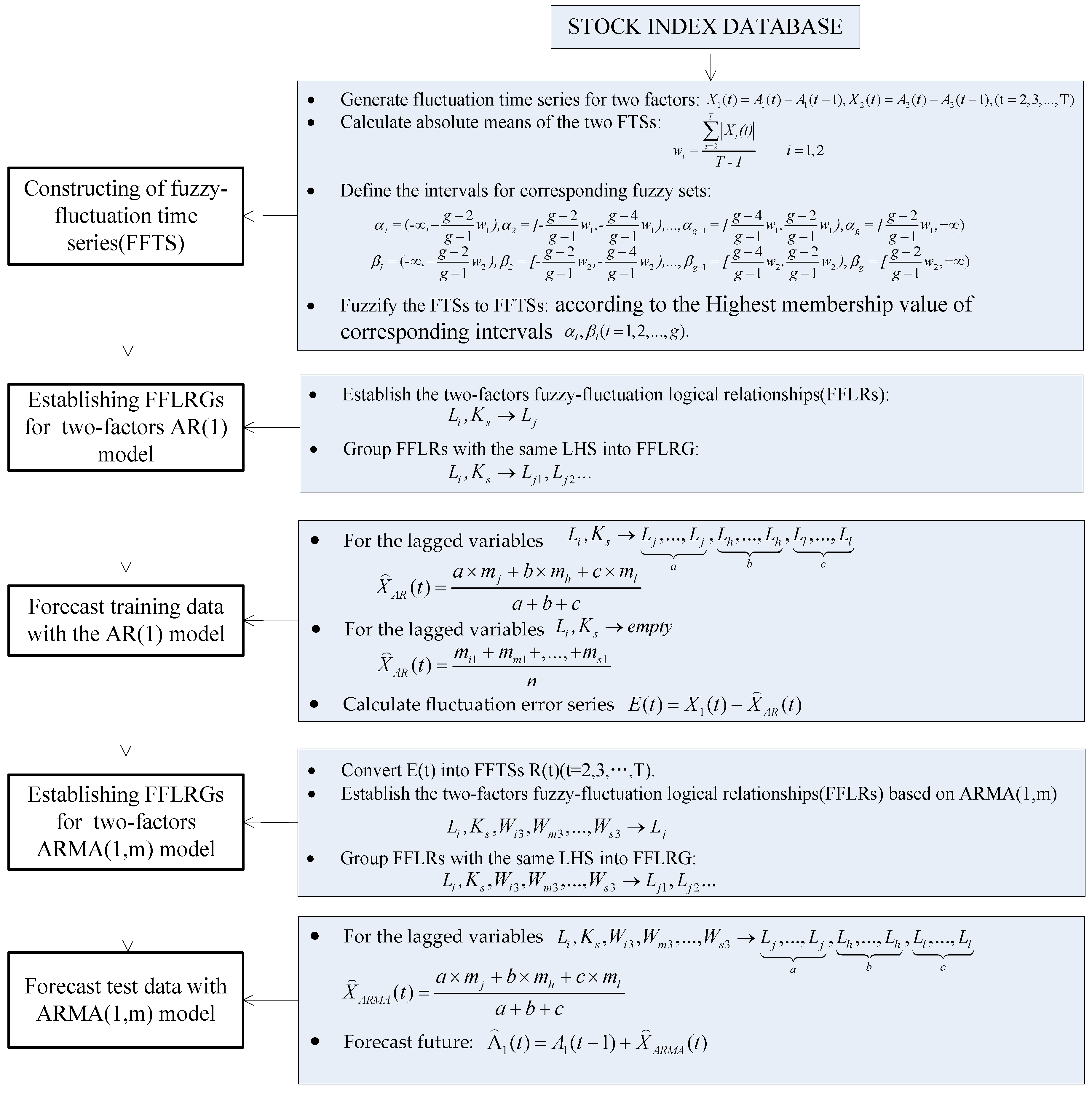
Figure 2.
Comparison of actual and forecast results for Taiwan Stock Exchange Capitalization Weighted Stock Index (TAIEX) test dataset (1997–2005). (X coordinate is the TAIEX and Y coordinate is the time series number remarked by “time(s)”.)
Figure 2.
Comparison of actual and forecast results for Taiwan Stock Exchange Capitalization Weighted Stock Index (TAIEX) test dataset (1997–2005). (X coordinate is the TAIEX and Y coordinate is the time series number remarked by “time(s)”.)
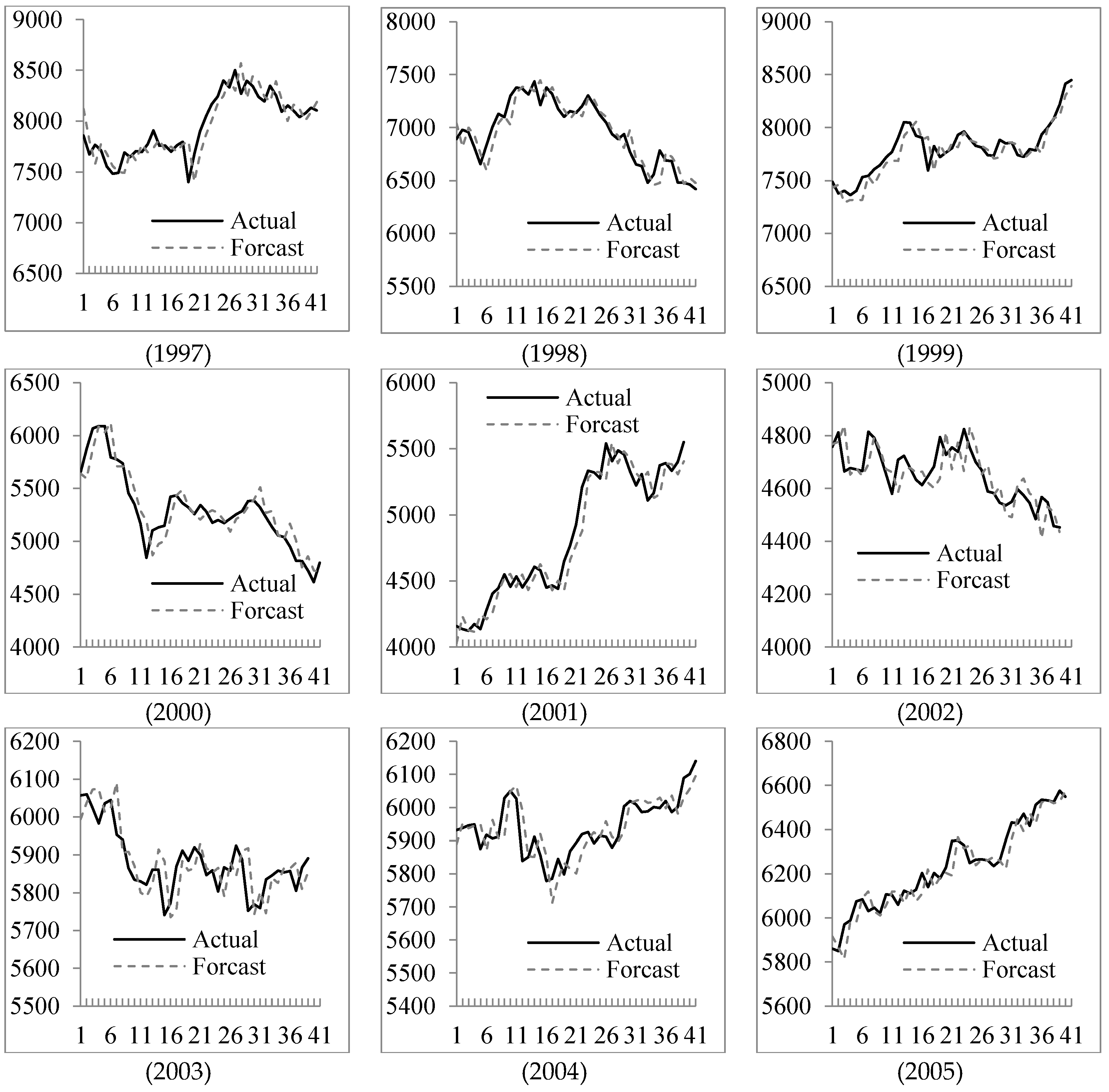
Figure 3.
Comparison of actual and forecast results for gold prices in 2010.

Table 1.
Fuzzy two-factor first-order autoregressive(AR(1)) solution.
| Fuzzy Value of Main Factor | Fuzzy Value of Secondary Factor | Fuzzy Forecast | Defuzzified Forecast |
|---|---|---|---|
| 1 | 1 | 2,1,5,5,1,1,5,5,3,1,5,3,1,5,3,5,2,1, | 0 |
| 1 | 2 | 4,3,1, | −11.17 |
| 1 | 3 | 1,1,5,4,1,3,2,3,5,5, | 0 |
| 1 | 4 | 5,1,4,4,3, | 13.4 |
| 1 | 5 | 3,2,1,5,1,1,5,5,3, | −3.72 |
| 2 | 1 | 1,4,5,1,5,2,3,2, | −4.19 |
| 2 | 2 | 4,3,1,1, | −25.13 |
| 2 | 3 | 5,5,3,3,5,3,3,3,2,5,5, | 27.41 |
| 2 | 4 | 1,4, | −16.75 |
| 2 | 5 | 4,4,3,2,5,3, | 16.75 |
| 3 | 1 | 2,3,2,1,1,5,4,1,5,4,5,1,5,5,1,3, | 0 |
| 3 | 2 | 3,4,3,2,2, | −6.7 |
| 3 | 3 | 2,4,3,5,5,1,4,2,1, | 0 |
| 3 | 4 | 3,5,1,5,2,3,3,2,3,1,4, | −3.05 |
| 3 | 5 | 1,5,5,2,5,5,4, | 28.71 |
| 4 | 1 | 3,1,1,3,5,2,5,1,2, | −14.89 |
| 4 | 2 | 5,3,1,1,5,4, | 5.58 |
| 4 | 3 | 3,1,2,3, | −25.13 |
| 4 | 4 | 2,5, | 16.75 |
| 4 | 5 | 5,3,5,5,4,4, | 44.67 |
| 5 | 1 | 1,1,3,2,2,4,5,2,3,3,3, | −12.18 |
| 5 | 2 | 4,2,1,1, | −33.5 |
| 5 | 3 | 3,3,3,1,1,3,1,1,1,3,5,4, | −19.54 |
| 5 | 4 | 2,3,3,4,5,2,4, | 9.57 |
| 5 | 5 | 2,4,2,2,3,5,5,3,3,3,2,5,4,4,1,5,5,5,5, | 19.39 |
Table 2.
Forecasting results from 1 November 2004 to 31 December 2004.
| Date (MM/DD/YYYY) | Actual | Forecast | (Forecast–Actual)2 | Date (MM/DD/YYYY) | Actual | Forecast | (Forecast–Actual)2 |
|---|---|---|---|---|---|---|---|
| 11/05/2004 | 5931.31 | 5889.44 | 1753.10 | 12/06/2004 | 5919.17 | 5868.14 | 2604.06 |
| 11/08/2004 | 5937.46 | 5950.70 | 175.30 | 12/07/2004 | 5925.28 | 5904.28 | 441.00 |
| 11/09/2004 | 5945.20 | 5937.46 | 59.91 | 12/08/2004 | 5892.51 | 5925.28 | 1073.87 |
| 11/10/2004 | 5948.49 | 5945.20 | 10.82 | 12/09/2004 | 5913.97 | 5909.26 | 22.18 |
| 11/11/2004 | 5874.52 | 5948.49 | 5471.56 | 12/10/2004 | 5911.63 | 5958.64 | 2209.94 |
| 11/12/2004 | 5917.16 | 5870.80 | 2149.25 | 12/13/2004 | 5878.89 | 5911.63 | 1071.91 |
| 11/15/2004 | 5906.69 | 5961.83 | 3040.42 | 12/14/2004 | 5909.65 | 5895.64 | 196.28 |
| 11/16/2004 | 5910.85 | 5906.69 | 17.31 | 12/15/2004 | 6002.58 | 5926.40 | 5803.39 |
| 11/17/2004 | 6028.68 | 5910.85 | 13883.91 | 12/16/2004 | 6019.23 | 6012.15 | 50.13 |
| 11/18/2004 | 6049.49 | 6048.07 | 2.02 | 12/17/2004 | 6009.32 | 6019.23 | 98.21 |
| 11/19/2004 | 6026.55 | 6066.24 | 1575.30 | 12/20/2004 | 5985.94 | 6026.07 | 1610.42 |
| 11/22/2004 | 5838.42 | 5993.05 | 23910.44 | 12/21/2004 | 5987.85 | 6013.35 | 650.25 |
| 11/23/2004 | 5851.10 | 5851.82 | 0.52 | 12/22/2004 | 6001.52 | 6016.56 | 226.20 |
| 11/24/2004 | 5911.31 | 5851.10 | 3625.24 | 12/23/2004 | 5997.67 | 6030.23 | 1060.15 |
| 11/25/2004 | 5855.24 | 5920.88 | 4308.61 | 12/24/2004 | 6019.42 | 5997.67 | 473.06 |
| 11/26/2004 | 5778.65 | 5855.24 | 5866.03 | 12/27/2004 | 5985.94 | 6036.17 | 2523.05 |
| 11/29/2004 | 5785.26 | 5711.65 | 5418.43 | 12/28/2004 | 6000.57 | 5981.75 | 354.19 |
| 11/30/2004 | 5844.76 | 5785.26 | 3540.25 | 12/29/2004 | 6088.49 | 6029.28 | 3505.82 |
| 12/01/2004 | 5798.62 | 5832.58 | 1153.28 | 12/30/2004 | 6100.86 | 6054.99 | 2104.06 |
| 12/02/2004 | 5867.95 | 5815.37 | 2764.66 | 12/31/2004 | 6139.69 | 6094.16 | 2072.98 |
| 12/03/2004 | 5893.27 | 5800.95 | 8522.98 | RMSE | 53.05 |
Table 3.
Comparison of forecasting errors for different two-factor first-order autoregressive moving average (ARMA(1,m)) model (g = 5).
Table 3.
Comparison of forecasting errors for different two-factor first-order autoregressive moving average (ARMA(1,m)) model (g = 5).
| m | None | 1 | 2 | 3 | 4 | 5 |
|---|---|---|---|---|---|---|
| RMSE | 57.59 | 59.32 | 61.74 | 53.05 | 60.84 | 63.22 |
Table 4.
Comparison of forecasting errors for different linguistic sets (m = 3).
| g | 3 | 5 | 7 | 9 |
|---|---|---|---|---|
| RMSE | 57.25 | 53.05 | 58.99 | 65.8 |
Table 5.
RMSEs of forecast errors for TAIEX 1997 to 2005.
| Year | 1997 | 1998 | 1999 | 2000 | 2001 | 2002 | 2003 | 2004 | 2005 |
|---|---|---|---|---|---|---|---|---|---|
| RMSE | 130.9 | 111.95 | 101.11 | 127.47 | 114.19 | 61.92 | 53.05 | 53.07 | 52.27 |
Table 6.
A comparison of RMSEs for different methods for forecasting the TAIEX 2004.
| Methods | RMSE | ||||||
|---|---|---|---|---|---|---|---|
| 1999 | 2000 | 2001 | 2002 | 2003 | 2004 | Average | |
| Huarng et al.’s Method [41] | N/A | 158.7 ** | 136.49 ** | 95.15 ** | 65.51 ** | 73.57 ** | 105.88 |
| Chen and Chang’s Method [29] | 123.64 ** | 131.1 | 115.08 | 73.06 ** | 66.36 ** | 60.48 ** | 94.95 |
| Chen and Chen’s Method [30] | 119.32 ** | 129.87 | 123.12 | 71.01 | 65.14 ** | 61.94 ** | 95.07 |
| Chen et al.’s Method [42] | 102.34 | 131.25 | 113.62 | 65.77 | 52.23 | 56.16 | 86.89 |
| Cheng et al.’s method [43] | 100.74 | 125.62 | 113.04 | 62.94 | 51.46 | 54.24 | 84.68 |
| Chen and Kao’s method [44] | 87.63 | 125.34 | 114.57 | 76.86 ** | 54.29 | 58.17 | 86.14 |
| Yu and Huarng’s method [45] | N/A | 149.59 ** | 98.91 | 78.71 ** | 58.78 | 55.91 | 88.38 |
| The Proposed Method | 101.11 | 127.47 | 114.19 | 61.92 | 53.05 | 53.07 | 85.14 |
** Use Diebold-Mariano test statistic (S), the proposed method has better accuracy than other methods at 5% significance level at least.
Table 7.
Root of the mean squared error (RMSE)s of forecast errors for Shanghai Stock Exchange Composite Index (SHSECI) from 2007 to 2015.
Table 7.
Root of the mean squared error (RMSE)s of forecast errors for Shanghai Stock Exchange Composite Index (SHSECI) from 2007 to 2015.
| Year | 2001 | 2002 | 2003 | 2004 | 2005 | 2006 | 2007 | 2008 | 2009 | 2010 | 2011 | 2012 | 2013 | 2014 | 2015 |
|---|---|---|---|---|---|---|---|---|---|---|---|---|---|---|---|
| RMSE | 24.86 | 21.75 | 26.57 | 19.07 | 9.63 | 28.98 | 129.22 | 79.77 | 59.96 | 49.48 | 29.7 | 23.14 | 22.13 | 44.11 | 58.89 |
Table 8.
RMSEs of forecast errors for gold price from 2000 to 2010.
| Year | 2000 | 2001 | 2002 | 2003 | 2004 | 2005 | 2006 | 2007 | 2008 | 2009 | 2010 |
|---|---|---|---|---|---|---|---|---|---|---|---|
| RMSE | 1.27 | 1.52 | 2.33 | 2.81 | 3.34 | 6.65 | 5.44 | 11.48 | 19.81 | 14.61 | 14.33 |
© 2017 by the authors. Licensee MDPI, Basel, Switzerland. This article is an open access article distributed under the terms and conditions of the Creative Commons Attribution (CC BY) license (http://creativecommons.org/licenses/by/4.0/).
Share and Cite
MDPI and ACS Style
Guan, S.; Zhao, A. A Two-Factor Autoregressive Moving Average Model Based on Fuzzy Fluctuation Logical Relationships. Symmetry 2017, 9, 207. https://doi.org/10.3390/sym9100207
AMA Style
Guan S, Zhao A. A Two-Factor Autoregressive Moving Average Model Based on Fuzzy Fluctuation Logical Relationships. Symmetry. 2017; 9(10):207. https://doi.org/10.3390/sym9100207
Chicago/Turabian StyleGuan, Shuang, and Aiwu Zhao. 2017. "A Two-Factor Autoregressive Moving Average Model Based on Fuzzy Fluctuation Logical Relationships" Symmetry 9, no. 10: 207. https://doi.org/10.3390/sym9100207
Note that from the first issue of 2016, this journal uses article numbers instead of page numbers. See further details here.