
Interference Alignment Based on Rank Constraint in MIMO Cognitive Radio Networks


1
College of Information and Communication Engineering, Harbin Engineering University, Harbin 150001, China
2
State Key Laboratory of the Gas Disaster Detecting Preventing and Emergency Controlling, Chongqing Research Institute of China Coal Technology and Engineering Group Corporation, Chongqing 400000, China
3
School of electrical and control engineer, Heilongjiang University of Science and Technology, Harbin 150022, China
*
Author to whom correspondence should be addressed.
†
Current address: College of Information and Communication Engineering, Harbin Engineering University, Harbin 150001, China
‡
These authors contributed equally to this work.
Symmetry 2017, 9(7), 107; https://doi.org/10.3390/sym9070107
Submission received: 29 April 2017
/
Revised: 23 June 2017
/
Accepted: 29 June 2017
/
Published: 4 July 2017
Abstract
:In this paper, we focus on the interference management in the cognitive radio (CR) network comprised of multiple primary users (PUs) and multiple secondary users (SUs). Firstly, two interference alignment (IA) schemes are proposed to mitigate the interference among PUs. The first one is an interference rank minimization (IRM) scheme, which aims to minimize the rank of the joint interference matrix via alternating between the forward and reverse communication links. Considering the overhead of information exchanged between the transmitters and receivers in the IRM scheme, we further develop an interference subspace distance minimization (ISDM) scheme which runs at the transmitters only. The ISDM scheme focuses on aligning the subspaces spanned by interference with an aligned subspace introduced in this paper. For the secondary network, though IRM and ISDM mitigate the received interference at secondary receivers, they make no attempt to eliminate the interference from SUs to PUs. To address this, we improve the IRM and ISDM schemes by putting a rank constraint into their optimizations, where the rank constraint forces the ranks of the interference matrices from SUs to PUs to be zero. Simulation results validate the effectiveness of the proposed schemes in terms of the average sum rate.
1. Introduction
With the rapidly increasing data rate requirements of mobile users for multimedia applications, the accessible radio spectrum is becoming critically scarce. Under traditional fixed spectrum allocation policy, some licensed bands are overcrowded while many others are underutilized. To address this issue, the cognitive radio (CR) concept was introduced to improve spectral efficiency in wireless systems. CR allows secondary users (cognitive users or SUs) to share the spectrum with the primary users (non-cognitive users or PUs) under the condition that SUs do not degrade the performance of PUs [1,2]. Dealing with the interference in the CR network is a challenging problem. Recently, an effective interference management scheme called interference alignment (IA) has been exploited to solve the interference problem in CR network [3].
Interference alignment (IA) is a recent breakthrough in approaching the capacity of interference networks at a high signal-to-noise ratio (SNR). To perform IA, several different algorithms with different properties are proposed. In [4], an iterative algorithm called interference leakage minimization (MWLI) was presented for the multiple-input multiple-output (MIMO) interference channel, which aimed to minimize the sum of interference power at each receiver. The authors proposed a rank constrained rank minimization (RCRM) in [5], which minimizes the nuclear norm of the interfering space with a full rank constraint on the desired signal space. Motivated by [5], a weighted version of nuclear norm minimization for finding the optimal encoders was further presented in [6]. In contrast to the above algorithms which perform their optimizations via alternating between the forward and reverse communication links, some one-sided algorithms for achieving IA at transmitters only were proposed in [7,8,9]. An IA scheme based on precoder design had been proposed in [7], where the precoders were chosen to minimize the sum of the smallest eigenvalues of interference covariance matrices over all receivers. In [8], the authors proposed designing the precoding matrices by minimizing the chordal distances of interfering subspaces. Apart from the above schemes, the feasibility conditions for IA in an interference channel were investigated in [10,11,12] whereby a rapid convergent IA scheme for wireless sensor networks was proposed.
So far, many works have studied applying IA to the CR networks [13,14,15,16,17,18,19,20,21,22,23]. In [13], the author characterized the achievable degree of freedom (DoF) for the secondary network. In [14], Zhou et al. optimized both the precoding vectors and power allocation to enhance the rates of secondary users, where a gradient method was used. In [15], under the presumption that the interference imposed by PU at each SU can be neglected, an IA scheme minimizing the distance between the interfering subspace and the received subspace was proposed. The authors of [16] proposed a maximum eigenmode beamforming (MEB) scheme applied to PUs, where the PU transmits its data only at the largest eigenmode and more unused eigenmodes can be reserved than in the water-filling algorithm. Inspired by [16], the authors in [17] proposed an eigenmode constraint with which the number of eigenmodes used by PUs was adaptively adjusted by the rate requirement. In [18], a space-time opportunistic IA technique was proposed for the overlay CR network, where the PU used space-time water-filling algorithm to optimize its transmission and in the process, freed up unused eigenmodes that could be exploited by the SU. The authors of [20] proposed an algorithm that enables the secondary transmitter to learn the interference channel of the primary receiver by measuring a monotonic function of the interference to the primary receiver. The authors of [21] put forward a blind opportunistic IA method with which the SU is able to compute blindly the required channel state information (CSI) without interaction with the primary network. In contrast to the above algorithms concentrating on the CR network with one PU and multiple SUs, the authors of [22,23] investigated the interference mitigation for the CR network with multiple PUs and multiple SUs. In [22], the authors presented an improved version of a minimum weighted leakage interference (IMWLI) algorithm with a much faster convergence rate. Authors of [23] developed an optimal interference elimination solution when there are sufficient antennas in the secondary links. Compared to the system in which a PU coexists with multiple SUs, the multi-PU CR system needs to deal with more serious interference, in particular the interference between PUs and SUs. The most commonly-used scheme to eliminate the mutual interference between PUs and SUs is by removing some antennas from the SUs’ transmitters and receivers, as proposed in [22,23]. Although such an approach allows SUs to transmit their information without causing/receiving any interference to/from the primary links, it demands them to be equipped with more antennas when the number of PUs increases.
In this paper, we focus on the interference management in the CR network with multiple primary links and multiple secondary links. Firstly, we propose two IA algorithms to mitigate the interference among PUs. In a perfect IA scheme, the signals are constrained into the same subspace at the unintended receivers, and thus the desired signal can be recovered by eliminating the aligned interferences. Based on this point, an interference rank minimization (IRM) algorithm, which minimizes the rank of the joint interference matrix via alternating between the forward and reverse communication links, is proposed to reduce the dimensions occupied by the interference signals. Considering the overhead of information exchanged between the transmitters and receivers in the IRM scheme, we develop an interference subspace distance minimization (ISDM) scheme which performs its iteration at the transmitters with the local CSI. The ISDM scheme first introduces the concept of aligned subspace, and then reduces the interference dimensions via aligning the subspaces spanned by interference with the aligned subspace. For the secondary links, though the received interference at secondary receivers can be mitigated through IRM and ISDM, the proposed two IA schemes make no attempt to eliminate the interference from SUs to PUs. Therefore, IRM and ISDM cannot be directly used for the secondary network. To address this, we improve the IRM and ISDM scheme by putting a rank constraint into their optimizations, where the rank constraint forces the rank of the interference matrix from SU to PU to be 0. In this paper, the improved versions of IRM and ISDM for SUs are respectively defined as IRM based on the rank constraint (IRM-RC) and ISDM based on the rank constraint (ISDM-RC). It is worth mentioning that, compared with the commonly used method to eliminate interference from SUs to PUs, our rank constraint need not equip SUs with additional antennas with the increasing number of primary users. Simulation results show the effectiveness of the proposed schemes in terms of the average sum rate. We further validate that the proposed schemes can be applied to the system regardless of whether the antennas of secondary users are sufficient or not.
The rest of this paper is organized as follows. Section 2 introduces the system model. The details of IRM and ISDM are described in Section 3.1 and Section 3.2, respectively. Section 4 provides the IRM-RC and ISDM-RC schemes for secondary MIMO links. Simulation results are given in Section 5. The paper concludes in Section 6.
Notation: Throughout the paper, we use bold uppercase and lowercase letters to denote matrices and vectors respectively. , , , and denote the Hermitian transposition, rank, Frobenius norm, nuclear norm and trace of the matrix , respectively. denotes the distance between the two subspaces spanned by and . denotes a matrix whose columns constitute an orthonormal basis for the orthogonal complement of . is the smallest eigenvalue of . denotes the minimum eigenvalue of . stands for the identity matrix and stands for the null matrix. means is Hermitian positive definite. represents the statistical expectation.
2. System Model
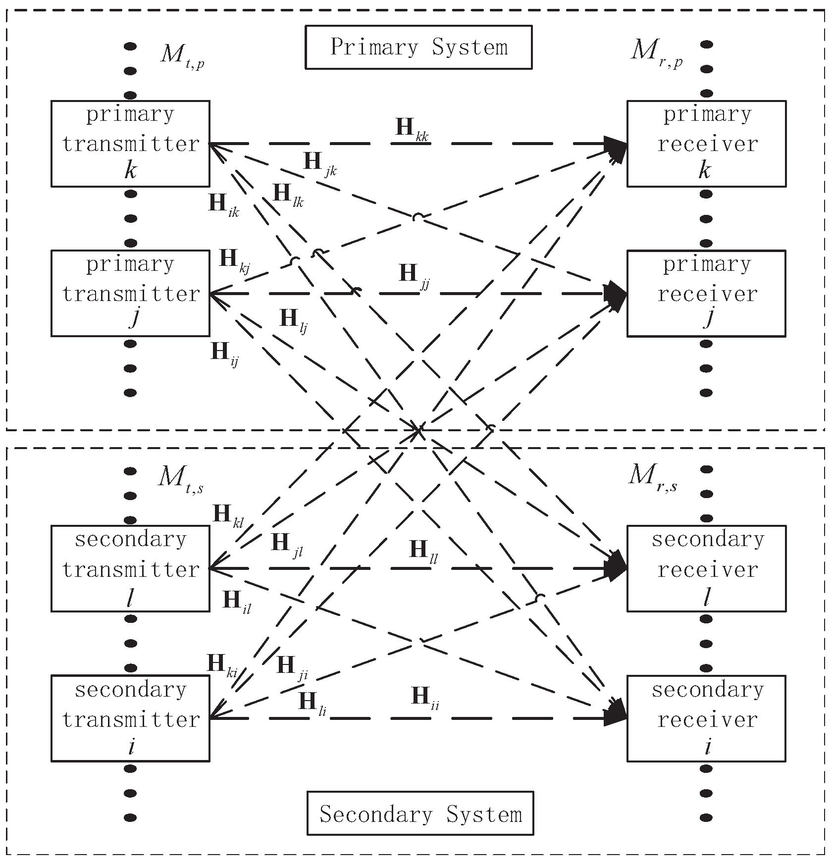
Consider a K-user MIMO-CR interference network as shown in Figure 1, which consists of PUs and SUs (). All the PUs and SUs share the same spectrum simultaneously.
The received signal at the k-th PU is given by:
The received signal at the l-th SU is given by:
and represent the transmitted signals from the k-th primary transmitter and the l-th secondary transmitter, respectively. Each PU sends independent data streams. denotes the independent data streams of the l-th SU. We assume that the transmitted signals are independently identically distributed (i.i.d). The transmitted power by the k-th primary transmitter is , where is the source covariance matrix. denotes the transmitted power by the l-th secondary transmitter, where represents the source covariance matrix. and are the zero mean unit variance circularly symmetric additive white Gaussian noise vectors. The definitions for the other symbols are provided in Table 1.
3. Proposed IA Schemes
Since primary users transmit their signals regardless of secondary users, the optimization problem in the primary network can be considered as a standard IA problem, and thus IA schemes can be directly applied to PUs. In this section, we focus on the alignment of the unintended signals for each PU, and two IA schemes aiming to reduce the dimensions occupied by the interference signals are proposed.
3.1. Interference Rank Minimization (IRM)
The space spanned by the interference signals at the k-th primary receiver is:
According to the matrix theory, the dimension of can be expressed as . To reduce the dimensions occupied by the interference signals, the objective for the IRM here can be modeled as minimizing the rank of the joint interference matrix as shown in Equation (4).
To approach this highly nonconvex and intractable problem in Equation (4), we use convex relaxations for the objective function [5]. Thus we have:
where denotes the convex envelope. The normalized nuclear norm in Equation (5) is the convex envelope of the rank of the joint interference matrix when the maximum singular value of the joint interference matrices is upper bounded by [24]. The optimization problem for the primary system is:
From the optimal solution, the majority of the interference experienced at the k-th primary receiver falls into the same subspace. Nevertheless, the received signal-to-interference-and-noise-ratio (SINR) could still have significant degradation if the desired signal subspace of the k-th primary user lies close to the interference subspace. Moreover, the decoder at the k-th primary receiver would not be completely orthogonal to the aligned interference subspace for the sake of improving received SINR. As a result, there may exist leaked interference power at the k-th primary receiver. It is enough to only minimize the rank of the joint interference matrix. To address this, we improve the rank optimization in Equation (6) through two steps:
The first step: We put the constraint on the desired power into the optimization problem.
where is the minimum desired power requirement.
Considering that the Frobenius norm is convex, we substitute the Frobenius norm in Equation (7) with the minimum eigenvalue which is concave for a real symmetric or complex Hermitian matrix.
where is the modified minimum desired power requirement.
Proof:
We force the desired signal matrix to be Hermitian positive definite. Using the identity that and , we obtain:
Since is an Hermitian positive definite matrix, its eigenvalues are all greater than zero. Using the Cauchy inequality, we derive:
From , we have:
☐
The second step: We improve the optimization problem in Equation (6) with a weighted optimization in order to mitigate the leaked interference power.
where () stands for the weighted value.
In view of the above two steps, we reformulate the optimization problem to a constrained one.
In this paper, we define:
The logical flow of the IRM algorithm is given as follows::
- Set and , start with arbitrary decoding matrices ;
- Calculate , according to Equation (3);
- If c is odd, solve,If c is even, solve,
- If , go to Step 5. If not, set , go to Step 2;
- Orthogonalize .
3.2. Interference Subspace Distance Minimization (ISDM)
Though IRM can effectively improve the system performance, its pre- and post-processing filter design needs to alternate between the forward and reverse communication links. Considering the overhead of information exchanged between the transmitters and receivers in the IRM scheme, we develop an interference subspace distance minimization (ISDM) scheme which runs at the transmitters only.
To reduce the interference dimensions at all receivers, one of the achievable methods is to minimize the sum of subspace distances between different interfering signals over all receivers. Since the total spatial distances in such an approach are approximate to , there exist excessive spatial distances to be optimized with the number of users increasing. To solve this problem, this paper introduces the concept of aligned subspace and reduces the interference dimensions via aligning the subspaces spanned by interference with the aligned subspace. It is not difficult to find that the spatial distances needed to be optimized in ISDM are approximate to at each transmitter.
Lemma 1.
Assume that there is a matrix and a linear subspace spanned by . According to the matrix theory, the orthogonal projection of onto the subspace spanned by is . Thus, the sum of the squared Euclidean distances between the columns of and their orthogonal projections onto the subspace spanned by can be expressed as .
We define as the k-th primary aligned matrix, whose columns span the k-th aligned subspace. Using lemma 1, the total sum of the spatial distances between the interference subspace and the aligned subspace in the secondary network is:
From , Equation (15) can be expressed as:
To solve the optimization problem in an iterative fashion, we first calculate . Intuitively, when taking as the variable, the items related to in Equation (16) are:
According to the matrix theory,
The optimal solution to the objective function in Equation (18) is:
where denotes the least significant eigenvectors of . Obviously, the calculation of can be only taken at the k-th transmitter node with local CSI.
Similarly, if we take as the variable, the items related to in Equation (16) are:
Note that the optimization problem in Equation (20) mitigates the interference on the undesired receiver while ignoring the distance between two subspaces spanned by the desired signal matrix and the aligned matrix. To alleviate this drawback, we put the constraint on the desired power into the optimization, which is similar to the method adopted to IRM:
Considering the precoders design is taken at the transmitters only, we substitute with columns of .
We reformulate the precoding matrix optimization problem as:
Note that the calculation of is also taken at the j-th primary transmitter with local CSI. In this paper, we define:
The logical flow of the precoders design in the ISDM algorithm is given as follows:
- Set and , start with arbitrary ;
- Calculate according to Equation (19);
- At the j-th primary transmitter,Solve:
- If , go to Step 5. If not, set , go to Step 2;
- Output: .
The receive filters have been totally excluded from the optimization problem so far. In the following, we illustrate the calculation of decoders. A sub-matrix optimization method is employed to design the primary decoders, where the primary decoding matrix is divided into two sub-matrices (). The first sub-decoder manages the interference from other PUs while the second sub-decoder improves the received desired signal power.
After achieving the optimal precoders, the subspaces spanned by interference from other PUs are almost aligned with the subspace spanned by the aligned matrix. We choose the orthogonal complement of as the first sub-decoder .
The intended signal power at the k-th primary receiver is:
In order to maximize the intended signal power, the columns of are chosen as the eigenvectors corresponding to the most significant eigenvalues of .
4. Interference Management in the Secondary Network
4.1. Rank Constraint Scheme
In this section, we study the issues for SUs. The CR network lets a complete secondary system operate in the same frequency band as the PUs such that no degradation is created for the PUs, i.e.,
The most commonly used scheme to protect PUs from the interference imposed by SUs is by removing some antennas from the SUs’ transmitters [22]. However, such an approach demands SUs to be equipped with additional antennas when the number of primary users increases, as shown in Equation (27).
To alleviate this drawback, we propose a rank constraint method to eliminate the interference generated to PUs, where SUs do not need to meet the antenna requirement in Equation (27). Since the matrix with rank 0 is a zero matrix, we have:
From Equation (28), the interferences from SUs to PUs can be controlled by a rank constraint:
Similar to what we have done previously, we replace the rank constraint with the nuclear norm constraint.
4.2. IRM Based on the Rank Constraint (IRM-RC)
An SU in the CR network suffers not only the interference imposed by other SUs but also the interference coming from PUs. The space spanned by the interference signals at the l-th secondary receiver is:
The received interference power at the l-th secondary receiver is:
The IRM algorithm cannot be directly used in the secondary network due to the fact that it makes no attempt to eliminate the interference generated on PUs by SUs. To achieve the goal of improving the secondary network performance without generating interference on the primary network, we improve IRM through putting the constraint in Equation (30) into the optimization of IRM, and refer this improved version as IRM-RC. The optimization problem of IRM-RC is expressed as:
In this paper, we define:
The logical flow of the IRM-RC algorithm is given as follows:
4.3. ISDM Based on the Rank Constraint
We define as the secondary aligned matrix, whose columns span the l-th secondary aligned subspace. For the secondary network, the total sum of the distances between the interference subspace and the aligned subspace is expressed as:
The optimal solution of is:
If we take as the variable, according to ISDM, the optimization problem is:
ISDM cannot be directly used for the secondary network due to the fact that it does not consider the constraint imposed on SUs by PUs as shown in Equation (26). Thus, in this section, we present an improved version of ISDM, called ISDM based on the rank constraint (ISDM-RC), where the CR interference to PUs are controlled by the constraint in Equation (30). The optimization problem with the rank constraint at the i-th transmitter is:
In this paper, we define:
The logical flow of the ISDM-RC algorithm is given as follows:
The sub-matrix optimization method is also adopted to calculate the secondary decoders. Since the details have been shown in Section 3.2, here, we just give the solution: The first sub-decoder is the orthogonal complement of ; The columns of are the eigenvectors corresponding to the most significant eigenvalues of .
5. Simulation
In this section, we provide some simulation examples to evaluate the performances of the proposed algorithms. The secondary system is represented by . In this paper, if and satisfy:
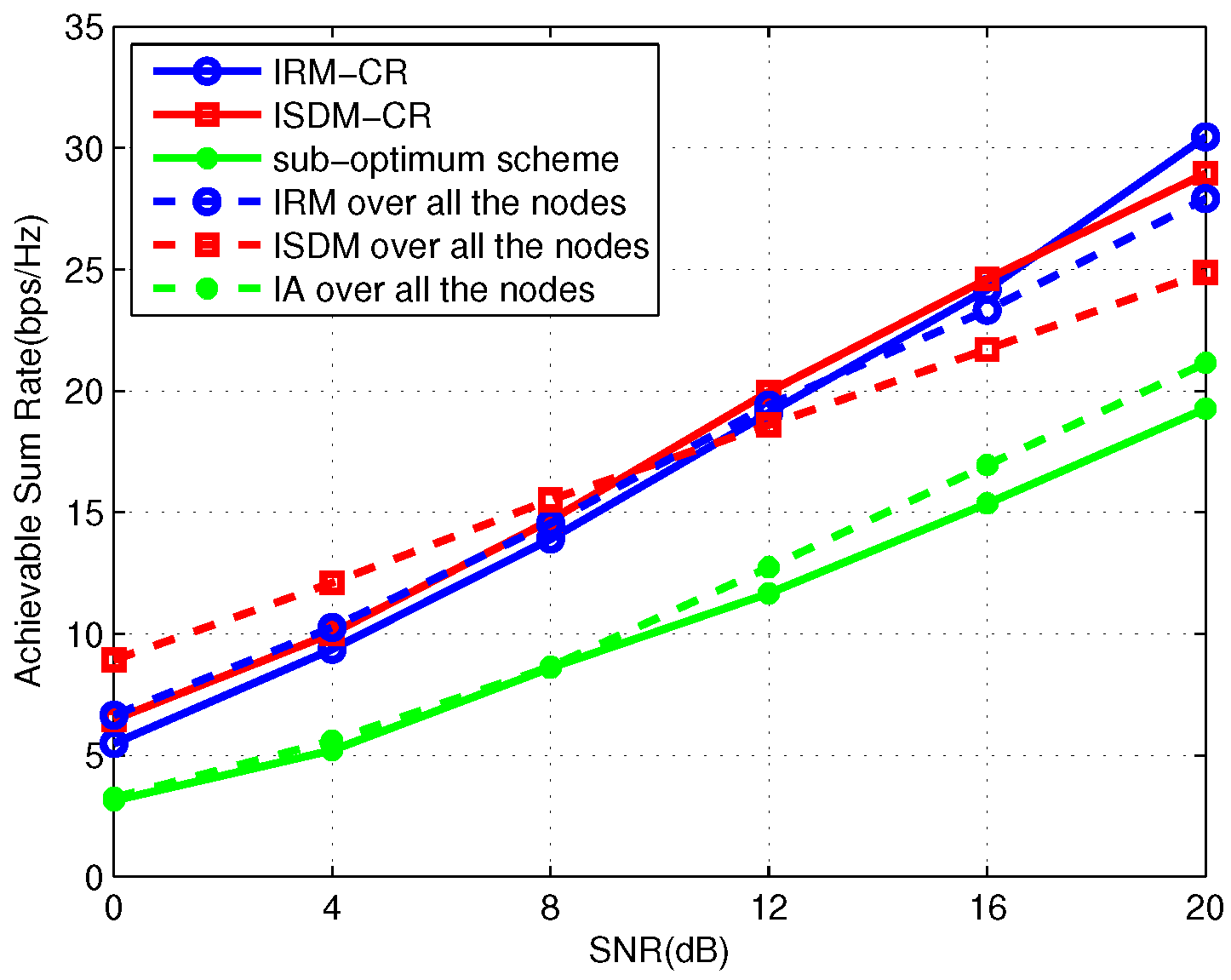
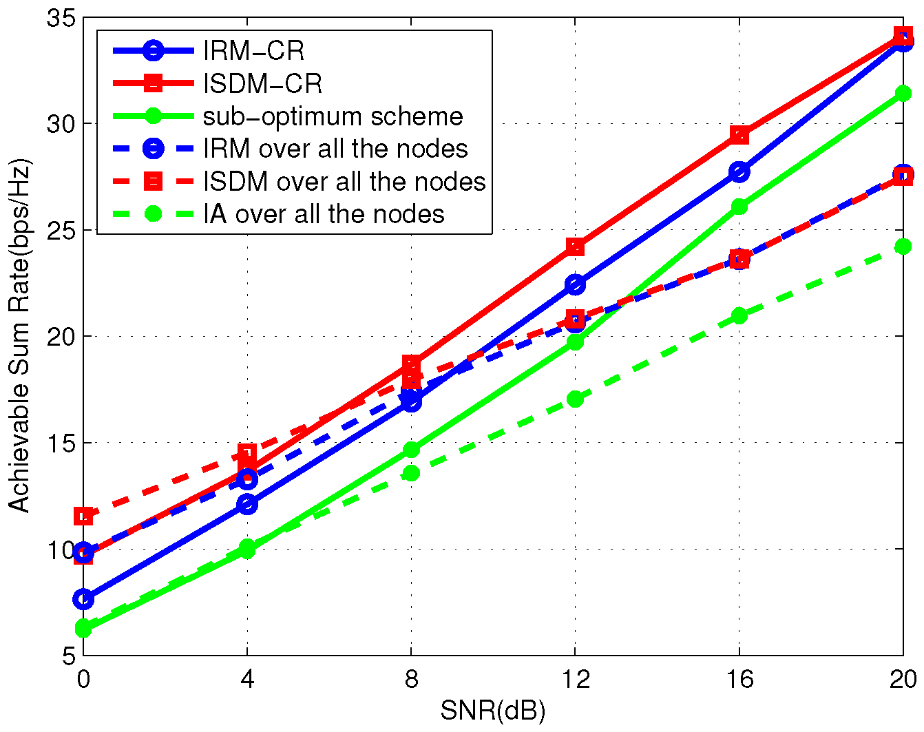
the secondary system is defined as an “adequate antennas system”; otherwise, the secondary system is defined as an “inadequate antennas system”. Simulation results are averaged over 500 channels. The noise power is normalized to one. equals to 0.1 [5]. is 0.02 [6]. The optimization problems proposed in this paper are all solved by the CVX toolbox [25]. In the following, we first evaluate and compare the performance of the interference rank minimization in the CR network (IRM-CR) and interference subspace distance minimization in the CR network (ISDM-CR). sub-optimum scheme proposed in [23], “IRM over all the nodes”, “ISDM over all the nodes” and “IA over all the nodes” in the “inadequate antennas system”. IRM-CR means using IRM for PUs and IRM-RC for SUs. Similarly, ISDM-CR means applying ISDM to the primary network and ISDM-RC to the secondary links. The algorithm to deal with interference in the “inadequate antennas system” proposed in [23] is represented as a sub-optimum scheme. “IRM over all the nodes” means all the users are cooperating through the IRM IA schemes. Similarly, “ISDM over all the nodes” denotes all the users are cooperating through ISDM. “IA over all the nodes” means all the users are cooperating through the MWLI algorithm.
In Figure 2, Figure 3 and Figure 4, a symmetric three-user primary system with 4 transmit antennas and 2 receive antennas is considered, where each PU demands one DoF. We simulate the average total sum rate of the primary and secondary links where the secondary system is in Figure 2. As seen from the figure, the performance of IRM-CR is lower than that of ISDM-CR in the low SNR region, whereas it increases gradually and approaches the ISDM-CR curve when SNR is greater than 12 dB. Though IRM-CR achieves the same rate as ISDM-CR for SNRs greater than 12 dB, ISDM-CR is still considered to be superior to IRM-CR due to the one-sided precoders design in ISDM-CR. According to [23], the secondary precoding matrices design in the sub-optimum scheme only aims to mitigate interference from SU to PUs. For a system with multiple secondary users, it is very difficult to align the interference signals processed by the precoding matrices in the sub-optimum scheme into the same space direction. As a result, the interference among SUs can lead to poor performance of the secondary system, as confirmed through simulation.
Observing Figure 2, for SNRs lower than 16 db, “IRM over all the nodes” and “ISDM over all the nodes” respectively achieve a higher sum rate compared with IRM-CR and ISDM-CR. This is because PUs in the IRM-CR and ISDM-CR schemes design their pre- and post-processing matrices without any cooperation with SUs, whereas all the users are cooperating through IA in “IRM over all the nodes” and “ISDM over all the nodes”. Furthermore, SUs are constrained by the condition in Equation (26). Nevertheless, with the SNR increasing, IRM-CR and ISDM-CR respectively outperform “IRM over all the nodes” and “ISDM over all the nodes”. As know, SUs are treated fairly in “IRM over all the nodes” and “ISDM over all the nodes”, whereas they are treated unfairly in IRM-CR and ISDM-CR due to the fact that the primary network dominates in the CR network. Thus, the significant improvement of the IRM-CR and ISDM-CR schemes is attributed to the reduction of user fairness. Furthermore, it can be also observed that the performance improvement at the expense of user fairness reduction becomes more obvious with the SNR increasing.
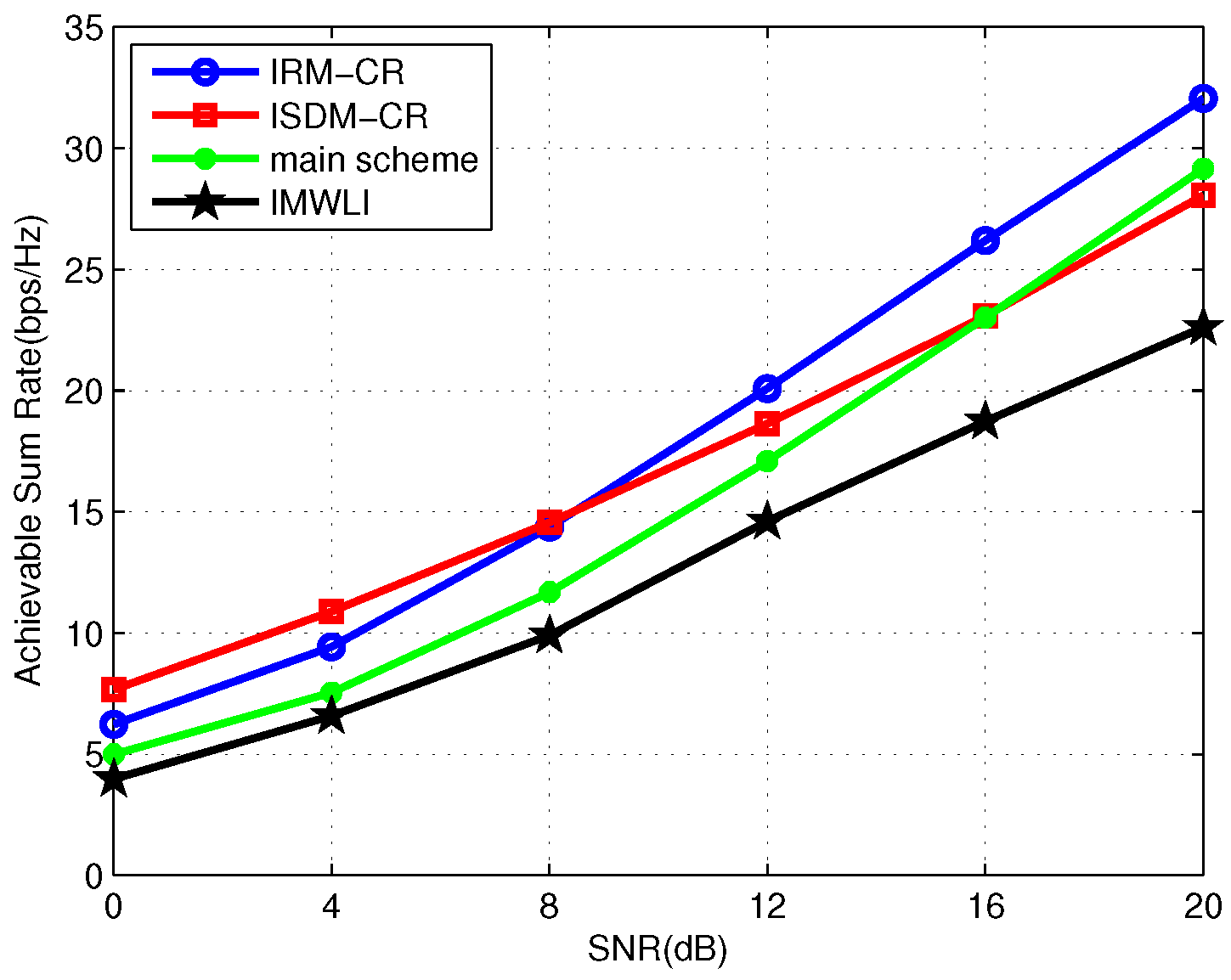
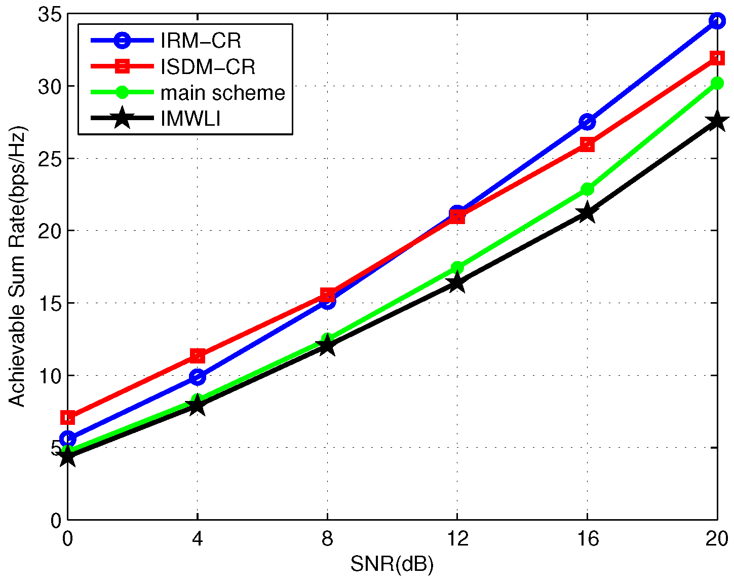
Figure 3 and Figure 4 simulate the average total sum rate of the primary and secondary links where the secondary system is and , respectively. Observing the two figures, under the same preexisting primary links, IRM-CR outperforms ISDM-CR by over 16 dB in the two-user secondary system and 4 dB in the three-user secondary system. It can be inferred that IRM-CR is superior to ISDM-CR when the number of SUs increases. In Figure 5, we consider a symmetric four-user primary network with four transmit antennas and two receive antennas. Each PU demands one DoF. The secondary system is . The transmission rate in the IRM-CR scheme is about 5 bps/Hz higher than ISDM-CR. Compared with Figure 3, it can be inferred that the increase of primary users can significantly influence the performance of the secondary links when applying ISDM-CR.
We consider a symmetric three-user primary system with antennas. Each PU demands two DoF. Figure 6 gives the average total sum rate of the primary and secondary links where the secondary system is . Under the same antenna configuration, Figure 7 displays the result that all SUs achieve two DoFs. Observing Figure 6, IRM-CR and ISDM-CR present a similar performance for SNRs, of lower than 16 db. As shown in Figure 7, the ISDM-CR scheme benefits from higher transmission rates compared with the IRM-CR approach. From these two figures, it is clear that ISDM-CR is more effective to mitigate interference than IRM-CR with an increasing number of DoFs.
In the following, we investigate the performance of IRM-CR, ISDM-CR in the “adequate antennas system”. Moreover, the main scheme proposed in [23] and the IMWLI algorithm are also considered, where the algorithm proposed by [23] to manage interference in the “adequate antennas system” is denoted as the main scheme. A symmetric three-user primary system with antennas is considered in Figure 8 and Figure 9, where each PU demands one DoF. Different from the above simulations, the two SUs in Figure 8 and Figure 9 are equipped with different antennas: the first one with five transmit/receive antennas and the second one with seven transmit/receive antennas.
In Figure 8, the first SU demands two DoFs while the second SU transmits one data stream. It can be seen that the ISDM-CR scheme has the best performance at the low SNR region while IRM-CR outperforms ISDM-CR with the SNR increasing. IMWLI achieves the worst performance. The sum rate achieved by the main scheme is higher than ISDM-CR when SNR is greater than 16 dB. According to [23], for a two-user secondary system, the first SU can maximize its data rate without degrading the performance of the PUs and receive harmful effects from the primary system if:
The second SU is able to transmit its data streams without causing/receiving any interference to/from the preexisting users (PUs and the first SU), as well as improve its performance if:
Based on Equation (41), it is clear that the first SU can eliminate the received interference. According to Equation (42), the second SU can maximize its data rate while eliminating the interference imposed by the preexisting users. Therefore, the main scheme performs well when the performance is dominated by interference. The average total sum rate of the primary and secondary links where all the secondary users achieve two DoFs is shown in Figure 9. Observing Figure 9, ISDM-CR achieves the best performance at the low-SNR region while IRM-CR benefits from higher transmission rates compared with the other three approaches. Since there are not enough antennas for secondary users to optimize their links, the performance obtained by the main scheme is poor in Figure 9.
From Figure 2, Figure 3, Figure 4, Figure 5, Figure 6, Figure 7, Figure 8 and Figure 9, it can be observed that IRM-CR outperforms ISDM-CR with the SNR increasing. Here, we analysis the reasons for the significant performance improvement of IRM-CR. One of the reasons is that the “rank minimization” in IRM-CR is a more straightforward method to increase the achievable DoFs which is important to improve the system performance in the high-SNR region. Besides, IRM-CR minimizes the interference signals power, which further mitigating the impact of interference.
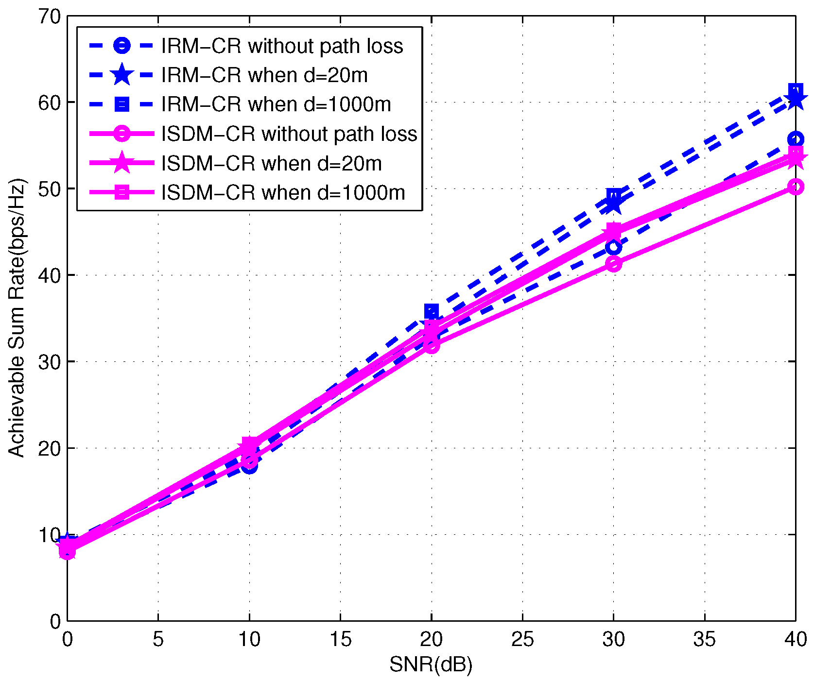
With the consideration of a number of parameters, the Cost-231 Walfisch-Ikagami model allows an excellent path loss model to explain the characters of an urban area. This model is appropriate for frequencies 800 MHz to 2000 MHz and distances ranging from 0.02 km to 5 km [26]. The path loss of this model is defined as:
where d and f respectively denote the distance in km and the frequency in MHz. Figure 10 gives the average total sum rate of the primary and secondary links where the Cost-231 Walfisch-Ikagami path loss model is used to estimate the path loss of the interfering links (PU-to-SU, SU-to-PU). We consider a symmetric three-user primary system with antennas. Each PU demands two DoF. The secondary system is . We can observe that the rate gets higher with the distance increasing under the large path loss environment. From the figure, the achievable rate is the lowest when the interfering links (PU-to-SU, SU-to-PU) have no large path loss, especially, when the performance is dominated by interference. However, the degradation of the rate without path loss is no more than 3 bps/Hz. We can infer that the proposed schemes can well eliminate the interference between the PU and the SU. Though the performance achieved by IRM-CR is higher than that of ISDM-CR, the ISDM-CR scheme is less sensitive to the path loss compared with the IRM-CR scheme.
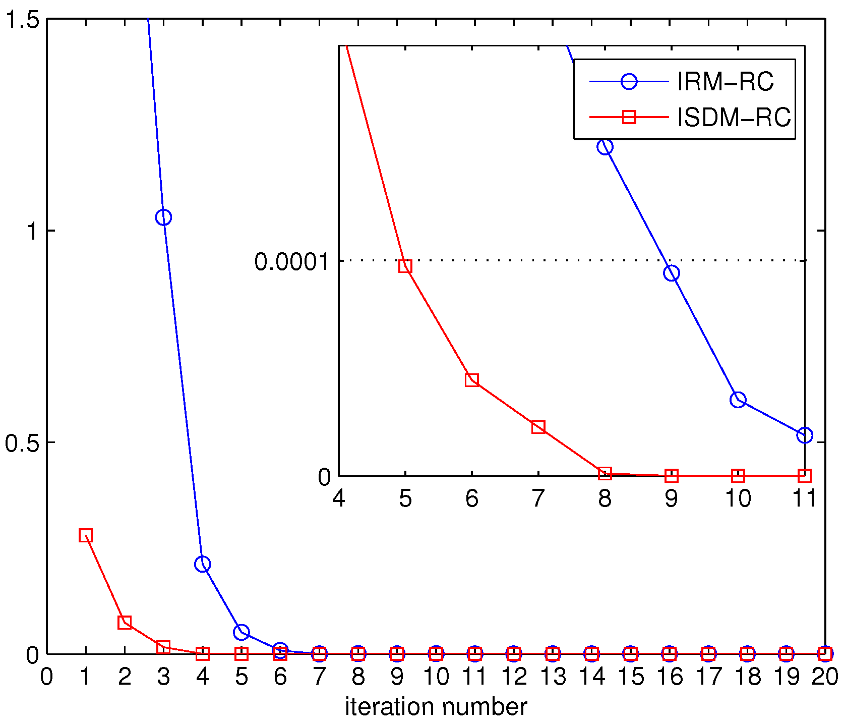
The previous figures show that the CR network achieves superior performances by applying proposed algorithms. We further evaluate the convergence of the proposed algorithms in Figure 11 and Figure 12. A primary network consisting of three primary users with antennas and a secondary network comprised of two secondary users with antennas are considered. Each user in the CR network demands two DoFs. In this paper, we focus on the difference of the objective function between two adjacent iterations. The convergence threshold is given as . Here, SNR = 15 dB. Figure 11 evaluates the convergence of IRM and ISDM. It can be seen that the difference of the objective function between the 11th and the 12th iteration is no more than 0.0001 in the ISDM scheme, whereas IRM needs 17 iterations to realize the objective function difference below 0.0001. In Figure 12, the convergence of IRM-RC and ISDM-RC is investigated in the presence of the primary network. To achieve the goal that the objective function difference between two adjacent iterations is lower than 0.0001, the IRM-RC approach needs nine iterations while the ISDM-RC requires five iterations. Observing Figure 11 and Figure 12, it is clear that the “spatial distances minimization” scheme converges faster than “rank minimization” scheme.
6. Conclusions
In this paper, PUs are cooperating through two proposed IA schemes. The first one is called IRM which aims to minimize the rank of the joint interference matrix. Since the optimizations based on alternating between the forward and reverse communication links in the IRM scheme generate additional overhead, we further develop an ISDM scheme which runs at the transmitters with the local CSI. The IRM and ISDM schemes cannot be directly used for the secondary network due to the fact that they make no attempt to eliminate the interference from SUs to PUs. To address this issue, we improve the two proposed schemes by putting a rank constraint into their optimizations, where the rank constraint forces the ranks of the interference matrix from SUs to PUs to be zero. Compared with the commonly used method protecting PUs from the interference imposed by SUs, our rank constraint does not need the secondary users to be equipped with additional antennas when the number of PUs increases. Simulation results show the proposed schemes can be applied to the system regardless of whether the transmit antennas of SUs are sufficient or not. We further validate that IRM-CR has a stronger ability to tackle the multiuser interference than ISDM-CR in the moderate to high SNR region.
Acknowledgments
This paper is funded by the National Natural Science Foundation of China (Grant No. 51509049), the National key research and development program (2016YFF0102806), and the Fundamental Research Funds for the Central Universities of China (Grant No. GK2080260140).
Author Contributions
The idea of this work was proposed by Yibing Li and Xueying Diao. Yibing Li and Xueying Diao performed the experiments and analyzed the simulation results. Qianhui Dong and Chunrui Tang assisted in the research work and wrote the paper.
Conflicts of Interest
The authors declare that there are no conflict of interests regarding the publication of this paper.
References
- Mitola, J.; Maquire, G.Q. Cognitive radio: making software radios more personal. IEEE Pers. Commun. 1999, 6, 13–18. [Google Scholar] [CrossRef]
- Goldsmith, A.; Jafar, S.A.; Mari’c, I.; Srinivasa, S. Breaking spectrum gridlock with cognitive radios: An information theoretic perspective. Proc. IEEE 2009, 97, 894–914. [Google Scholar] [CrossRef]
- Perlaza, S.M.; Fawaz, N.; Lasaulce, S.; Debbah, M. From spectrum pooling to space pooling: Opportunistic interference alignment in MIMO cognitive networks. IEEE Trans. Signal Process. 2010, 58, 3728–3741. [Google Scholar] [CrossRef]
- Gomadam, K.; Cadambe, V.R.; Jafar, S.A. A Distributed Numerical Approach to Interference Alignment and Applications to Wireless Interference Networks. IEEE Trans. Inf. Theory 2011, 57, 3309–3322. [Google Scholar] [CrossRef]
- Papailiopoulos, D.S.; Dimakis, A.G. Interference Alignment as a Rank Constrained Rank Minimization. IEEE Trans. Signal Process. 2012, 60, 4278–4288. [Google Scholar] [CrossRef]
- Du, H.; Ratnarajah, T.; Sellathurai, M.; Papadias, C. Reweighted nuclear norm approach for interference alignment. IEEE Trans. Commun. 2013, 61, 3754–3765. [Google Scholar] [CrossRef]
- Ghauch, H.G.; Papadias, C.B. Interference Alignment: A one-sided approach. In Proceedings of the IEEE Global Telecommunications Conference, Kathmandu, Nepal, 5–9 December 2011; pp. 1–5. [Google Scholar]
- Bazzi, S.; Dietl, G.; Utschick, W. Interference alignment via minimizing projector distances of interfering subspaces. In Proceedings of the IEEE International Workshop on Signal Processing Advances in Wireless Communications (SPAWC), Cesme, Turkey, 17–20 June 2012; pp. 274–278. [Google Scholar]
- Chen, H.; Zhou, Y.; Tian, L.; Liu, Z.; Ma, Y. Sum-rate improved interference alignment in wireless MIMO interference networks. In Proceedings of the IEEE Global Communication Conference (GLOBECOM), Austin, TX, USA, 8–12 December 2014; pp. 3366–3371. [Google Scholar]
- Yetis, C.M.; Tiangao, G.; Jafar, S.A.; Kayran, A.H. On feasibility of interference alignment in MIMO interference networks. IEEE Trans. Signal Process. 2010, 58, 4771–4782. [Google Scholar] [CrossRef]
- Ruan, L.; Lau, V.K.N.; Win, M.Z. The feasibility conditions for interference alignment in MIMO networks. IEEE Trans. Signal Process. 2013, 61, 2066–2077. [Google Scholar] [CrossRef]
- Jiang, L.H.; Wu, Z.L.; Ren, G.H.; Wang, G.Y.; Zhao, N. A Rapid Convergent Low Complexity Interference Alignment Algorithm for Wireless Sensor Networks. Sensors 2015, 15, 18526–18549. [Google Scholar] [CrossRef] [PubMed]
- Amir, M.; El-Keyi, A.; Nafie, M. Opportunistic interference alignment for multiuser cognitive radio. In Proceedings of the IEEE Information Theory Workshop on Information Theory (ITW 2010, Cairo), Cairo, Egypt, 6–8 January 2010; pp. 1–5. [Google Scholar]
- Zhou, H.; Ratnarajah, T.; Liang, Y. On secondary network interference alignment in cognitive radio. In Proceedings of the IEEE Symposium on New Frontiers in Dynamic Spectrum Access Networks (DySPAN), Aachen, Germany, 3–6 May 2011; pp. 637–641. [Google Scholar]
- Du, H.; Ratnarajah, T.; Zhou, H.; Liang, Y.C. Interference alignment for peer-to-peer underlay MIMO cognitive radio network. In Proceedings of the Asilomar Conference on Signals, Systems and Computers (ASILOMAR), Pacific Grove, CA, USA, 6–9 November 2011; pp. 349–353. [Google Scholar]
- Mosleh, S.; Abouei, J.; Aghabozorgi, M.R. Distributed opportunistic interference alignment using threshold-based beamforming in MIMO overlay cognitive radio. IEEE Trans. Veh. Technol. 2014, 63, 3783–3793. [Google Scholar] [CrossRef]
- Guo, W.; Xu, W.; Lin, J.; Fu, L. Adaptive eigenmodes beamforming and interference alignment in underlay and overlay cognitive networks. In Proceedings of the IEEE Annual International Symposium on Personal, Indoor, and Mobile Radio Communications, Hong Kong, China, 30 August–2 September 2015; pp. 798–802. [Google Scholar]
- Abdulkadir, Y.; Simpson, O.; Nwanekezie, N.; Sun, Y. Space-time opportunistic interference alignment in cognitive radio networks. In Proceedings of the IEEE Wireless Communications and Networking Conference, Doha, Qatar, 3–6 April 2016; pp. 1–6. [Google Scholar]
- Gao, F.; Zhang, R.; Liang, Y.C.; Wang, X. Design of Learning-Based MIMO Cognitive Radio Systems. IEEE Trans. Veh. Technol. 2010, 59, 1707–1720. [Google Scholar]
- Noam, Y.; Goldsmith, A.J. Blind Null-Space Learning for MIMO Underlay Cognitive Radio with Primary User Interference Adaptation. IEEE Trans. Wirel. Commun. 2013, 12, 1722–1734. [Google Scholar] [CrossRef]
- Tsinos, C.G.; Berberidis, K. Blind Opportunistic Interference Alignment in MIMO Cognitive Radio Systems. IEEE J. Emerg. Sel. Top. Circuits Syst. 2013, 3, 626–639. [Google Scholar] [CrossRef]
- Rezaei, F.; Tadaion, A. Interference alignment in cognitive radio networks. IET Commun. 2014, 8, 1769–1777. [Google Scholar] [CrossRef]
- Rezaei, F.; Tadaion, A. Sum-Rate Improvement in Cognitive Radio Through Interference Alignment. IEEE Trans. Veh. Technol. 2016, 65, 145–154. [Google Scholar] [CrossRef]
- Recht, B.; Fazel, M.; Parrilo, P. Guaranteed minimum rank solutions of matrix equations via nuclear Norm minimization. SIAM Rev. 2010, 52, 471–501. [Google Scholar] [CrossRef]
- Grant, M.; Boyd, S. CVX: Matlab Software for Disciplined Convex Programming; CVX Research, Inc.: Austin, TX, USA, 2009. [Google Scholar]
- Hu, Y.Q.; Zhao, Y.P.; Li, J.X.; Li, S.P.; Sun, C.; Guo, X. Channel measurements and modelling for cognitive radio devices with low-height antennas. In Proceedings of the IEEE International Conference on Communications in China, Shanghai, China, 13–15 October 2014; pp. 764–769. [Google Scholar]
Figure 1.
System model.

Figure 2.
Achievable rate of the system versus signal-to-noise ratio (SNR). IRM-CR: IRM-CR: Interference rank minimization in the CR network. ISDM-CR: interference subspace distance minimization in the CR network. IRM: Interference rank minimization. ISDM: Interference subspace distance minimization. IA: interference alignment.
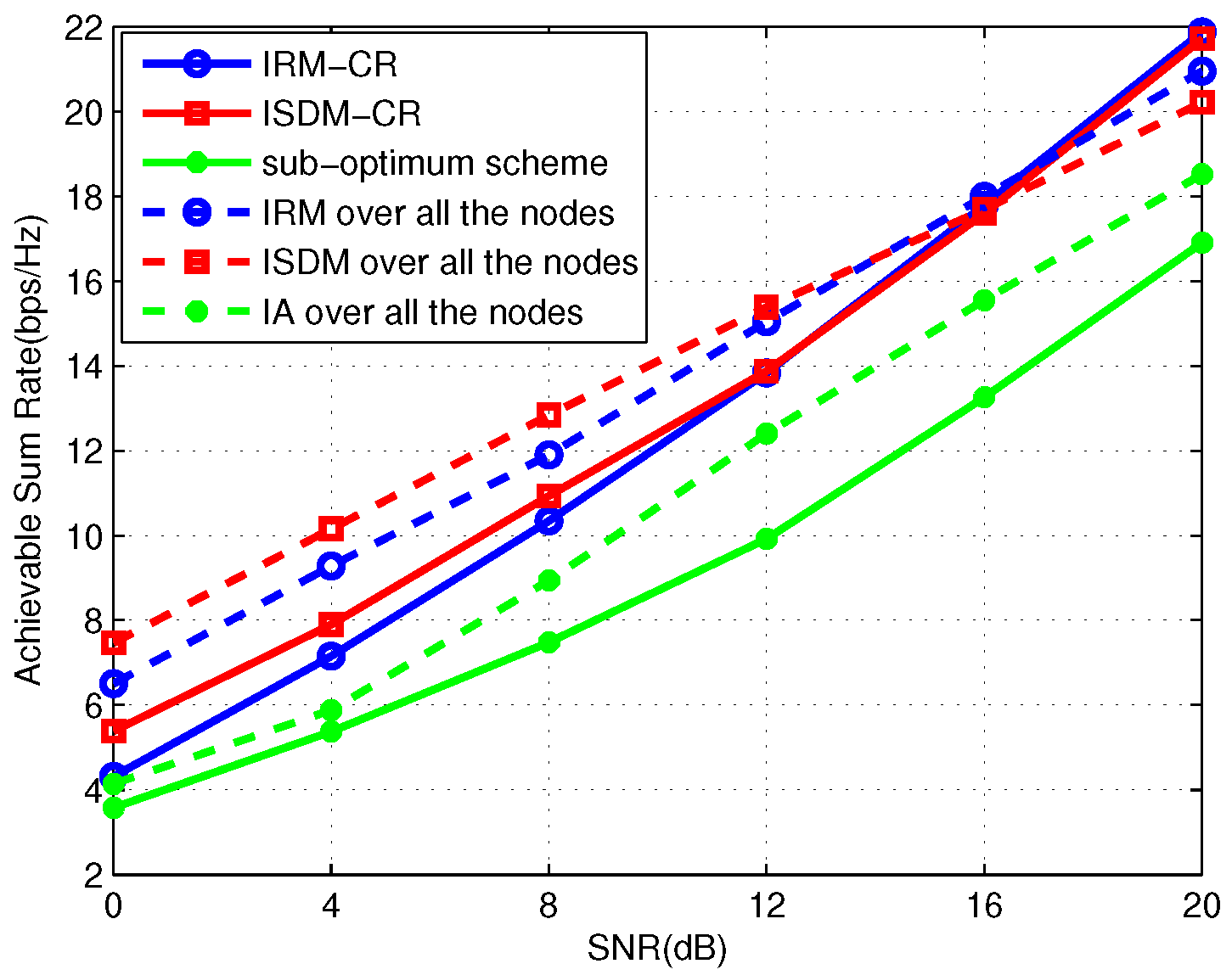
Figure 3.
Achievable rate of the system versus SNR.

Figure 4.
Achievable rate of the system versus SNR.
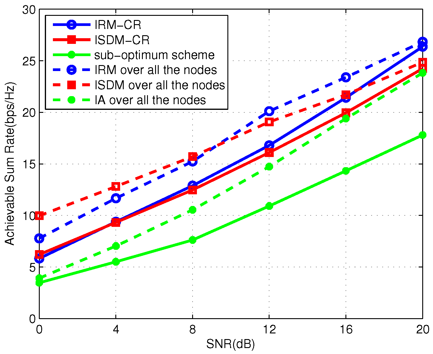
Figure 5.
Achievable rate of the system versus SNR.
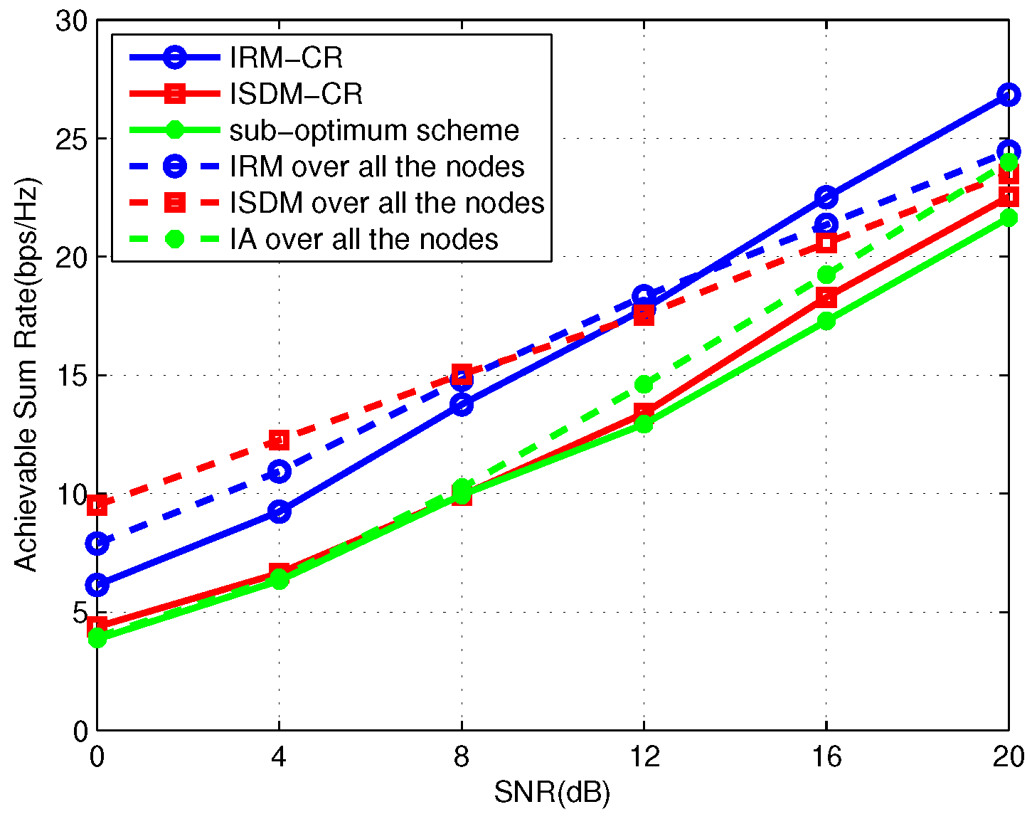
Figure 6.
Achievable rate of the system versus SNR.
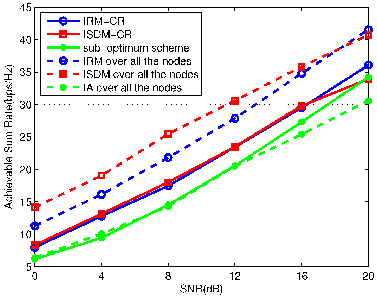
Figure 7.
Achievable rate of the system versus SNR.

Figure 8.
Achievable rate of the system versus SNR. IMWLI: improved version of a minimum weighted leakage interference.
Figure 8.
Achievable rate of the system versus SNR. IMWLI: improved version of a minimum weighted leakage interference.

Figure 9.
Achievable rate of the system versus SNR.

Figure 10.
Achievable sum rate under different path loss.

Figure 11.
Convergence of IRM and ISDM.
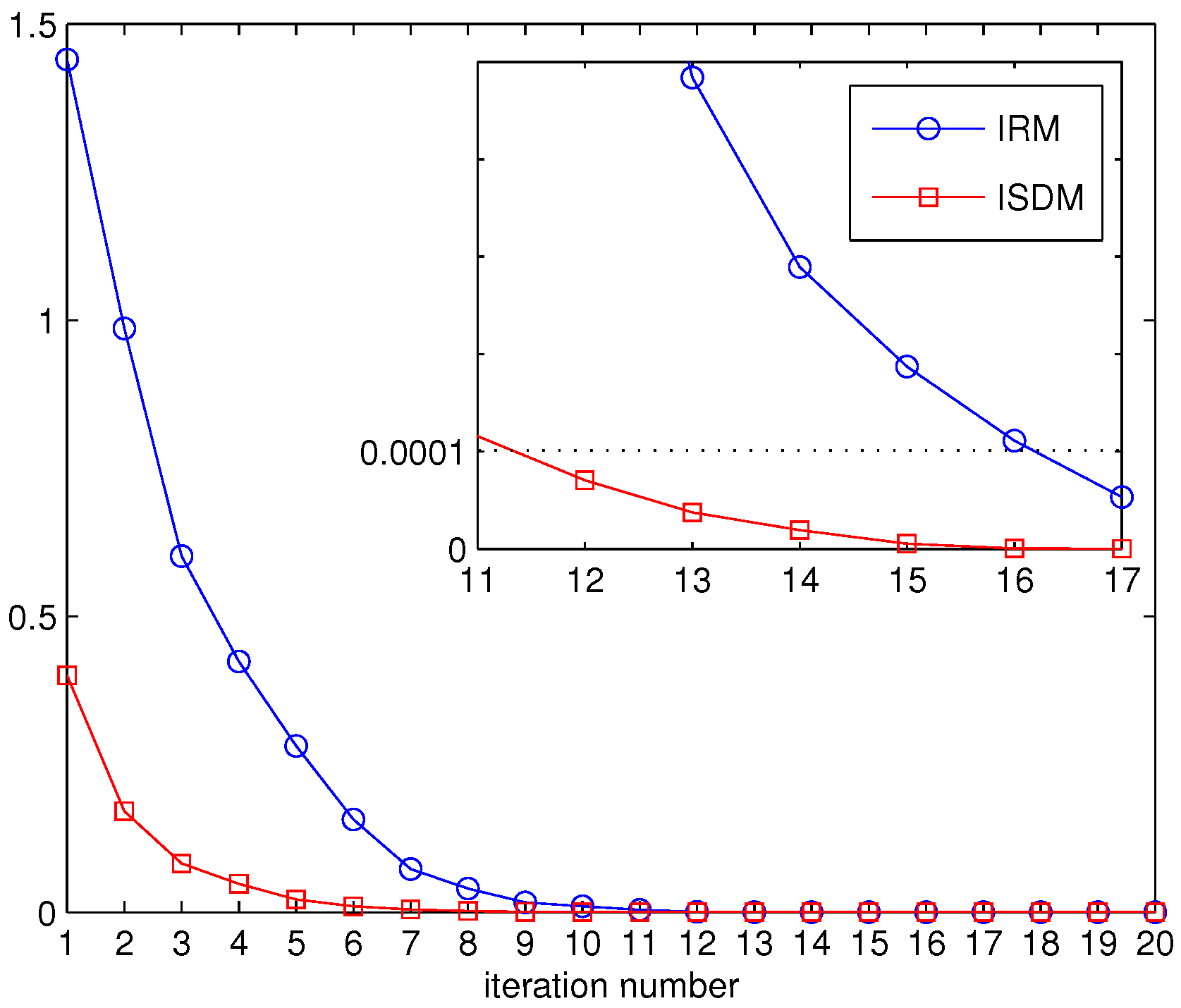
Figure 12.
Convergence of the IRM based on the rank constraint (IRM-RC) and the ISDM based on the rank constraint (ISDM-RC).
Figure 12.
Convergence of the IRM based on the rank constraint (IRM-RC) and the ISDM based on the rank constraint (ISDM-RC).

Table 1.
Symbol definitions. PU: primary user; SU: secondary user.
| Symbol | Definition |
|---|---|
| The number of PU transmit antennas | |
| The number of SU transmit antennas | |
| The number of PU receive antennas | |
| The number of SU receive antennas | |
| The precoding matrix of dimension at the k-th primary transmitter | |
| The decoding matrix of dimension at the k-th primary receiver | |
| The precoding matrix of dimension at the l-th secondary transmitter | |
| The decoding matrix of dimension at the l-th secondary receiver | |
| The channel coefficient between the k-th transmitter and its corresponding receiver | |
| The channel coefficient between the j-th transmitter and the k-th receiver |
© 2017 by the authors. Licensee MDPI, Basel, Switzerland. This article is an open access article distributed under the terms and conditions of the Creative Commons Attribution (CC BY) license (http://creativecommons.org/licenses/by/4.0/).
Share and Cite
MDPI and ACS Style
Li, Y.; Diao, X.; Dong, Q.; Tang, C. Interference Alignment Based on Rank Constraint in MIMO Cognitive Radio Networks. Symmetry 2017, 9, 107. https://doi.org/10.3390/sym9070107
AMA Style
Li Y, Diao X, Dong Q, Tang C. Interference Alignment Based on Rank Constraint in MIMO Cognitive Radio Networks. Symmetry. 2017; 9(7):107. https://doi.org/10.3390/sym9070107
Chicago/Turabian StyleLi, Yibing, Xueying Diao, Qianhui Dong, and Chunrui Tang. 2017. "Interference Alignment Based on Rank Constraint in MIMO Cognitive Radio Networks" Symmetry 9, no. 7: 107. https://doi.org/10.3390/sym9070107
Note that from the first issue of 2016, this journal uses article numbers instead of page numbers. See further details here.