Group Decision-Making for Hesitant Fuzzy Sets Based on Characteristic Objects Method

1
Department of Mathematics, University of Management and Technology, Lahore 54770, Pakistan
2
Department of Artificial Intelligence method and Applied Mathematics in the Faculty of Computer Science and Information Technology, West Pomeranian University of Technology, Szczecin, 71-210, Poland
3
Department of Web Systems Analysis and Data Processing in the Faculty of Computer Science and Information Technology, West Pomeranian University of Technology, Szczecin, 71-210, Poland
*
Author to whom correspondence should be addressed.
Symmetry 2017, 9(8), 136; https://doi.org/10.3390/sym9080136
Submission received: 28 June 2017
/
Revised: 15 July 2017
/
Accepted: 25 July 2017
/
Published: 29 July 2017
(This article belongs to the Special Issue Fuzzy Techniques for Decision Making)
Abstract
:There are many real-life problems that, because of the need to involve a wide domain of knowledge, are beyond a single expert. This is especially true for complex problems. Therefore, it is usually necessary to allocate more than one expert to a decision process. In such situations, we can observe an increasing importance of uncertainty. In this paper, the Multi-Criteria Decision-Making (MCDM) method called the Characteristic Objects Method (COMET) is extended to solve problems for Multi-Criteria Group Decision-Making (MCGDM) in a hesitant fuzzy environment. It is a completely new idea for solving problems of group decision-making under uncertainty. In this approach, we use L-R-type Generalized Fuzzy Numbers (GFNs) to get the degree of hesitancy for an alternative under a certain criterion. Therefore, the classical COMET method was adapted to work with GFNs in group decision-making problems. The proposed extension is presented in detail, along with the necessary background information. Finally, an illustrative numerical example is provided to elaborate the proposed method with respect to the support of a decision process. The presented extension of the COMET method, as opposed to others’ group decision-making methods, is completely free of the rank reversal phenomenon, which is identified as one of the most important MCDM challenges.
1. Introduction
For human activities and their problems, the Multi-Criteria Group Decision-Making (MCGDM) is an important tool [1,2]. In complex real-world conditions, it is not possible for a single Decision-Maker (DM) to recognize all of the relevant aspects of a decision-making problem [3]. Thus, the decision-making procedure requires considering many DMs or experts from different fields. In many group decision-making problems, a group is established by various DMs from different fields, including work experience, education backgrounds and knowledge structure [4]. It could be implemented to select the most suitable alternative from a given set of decision variants or their subset [5,6]. The essential prerequisite of the MCGDM is the combination of experts’ preferences and judgments about the candidate alternatives versus the conflicting criteria [7], which is a popular trend of present research to develop new group MCDM methods [8,9,10,11].
In the decision-making, the problems of uncertainty and hesitancy usually turn out to be unavoidable. To express the DMs’ evaluation information more objectively, several tools have been developed, such as fuzzy set [1,12], interval-valued fuzzy set [13,14], linguistic fuzzy set [15,16,17], which allow one to present an element’s membership function as a set denoted by a fuzzy number, an interval fuzzy number, a linguistic variable and a fuzzy set, respectively. Intuitionistic fuzzy set [18] and fuzzy multiset [19,20] are another two generalizations of the fuzzy set. Whilst the former contains three types of information (the membership, the non-membership and the hesitancy), the latter permits the elements to repeat more than once.
In many practical problems, sometimes, it is difficult to define the membership grade of an element, because of a set of possible membership values [21]. This issue is very important in MCGDM problems, when the DMs do not support the same membership grade for an element [22,23]. In this case, the difficulty of establishing a common membership grade is caused not by the margin of error (as happens in Intuitionistic Fuzzy Set (IFS)) or some possible distribution values (as happens in Type-2 Fuzzy Sets), but by the fact that several membership values are possible [10]. To deal with these cases, the Hesitant Fuzzy Set (HFS) was introduced [24] as a new generalization of fuzzy sets. Many MCDM methods have been extended by using the HFS theory, e.g., the ELECTRE family methods [25], Viekriterijumsko Kompromisno Rangiranje (VIKOR) [26] or prospect theory [27]. There was also established a number of new methods [13,28,29,30] or aggregation operators [31,32], which are based on the HFS concept. Presently, group decision-making problems are solved for hesitant fuzzy sets and with aggregation operators in [33,34,35,36]. Interval-valued hesitant fuzzy sets have been used in the applications of group decision-making in [28,37,38,39,40]. MCGDM with hesitant two-tuple linguistic information and by using trapezoidal valued HFSs is discussed in [41,42]. Yu [43] gave the concept of triangular hesitant fuzzy sets and used it for the solution of decision-making problems. Unfortunately, all of the mentioned group decision-making methods are susceptible to the occurrence of the rank reversal phenomenon paradox, which lies at the heart of the main MCDM challenges.
The Characteristic Objects Method (COMET) is a useful technique in dealing with Multi-Criteria Decision-Making (MCDM) problems [44,45,46,47,48]. It helps a DM to organize the structure of the problems to be solved and carry out the analysis, comparisons and ranking of the alternatives, where the complexity of the algorithm is completely independent of the alternatives’ number [49,50]. Additionally, comparisons between the Characteristic Objects (COs) are easier than comparisons between alternatives. However, the most important merit of the COMET method is the fact that this method is completely free of the rank reversals phenomenon [51] because the final ranking is constructed based on COs and fuzzy rules.
In this study, we extend the COMET concept to develop a methodology for solving multi-criteria group decision-making problems under uncertainty. The proposed method allows a group of DMs to make their opinion independent of linguistic terms by using HFS. The proposed method is designed for modeling uncertainty from different sources, which are related to expert knowledge. The main motivation of this research is the fact that the presented extension is also completely free of the rank reversals paradox as the classical version.
The group version of the HFS COMET method can be used in various research fields and disciplines such as economics [29,30,32], resource management [51], production [52], transport [53], game theory (Nash equilibrium) [54,55,56,57,58,59,60,61,62,63], medical problems [48,64], sustainability manufacturing [65] or web systems [66]; especially in decision situations requiring the involvement of many experts [67].
The rest of this paper is organized as follows. In Section 2, we introduced some basic concepts related to the hesitant fuzzy sets, L-R-type Generalized Fuzzy Numbers (GFNs), the fuzzy rule, the rule base and the t-norm. In Section 3, we established a group decision-making method based on COMET to deal with the uncertainty environment. In Section 4, an illustrative example is given to demonstrate the practicality and effectiveness of the proposed approach. Finally, we conclude the paper and give some remarks in Section 5.
2. Preliminaries
The HFS [24], as a generalization of the fuzzy set, maps the membership degree of an element to a set presented as several possible values between zero and one, which can better describe the situations where people have hesitancy in providing their preferences over objects in the process of decision-making.
In this section, we recall some important concepts that are necessary to understand our proposed decision-making method.
Definition 1.
A hesitant fuzzy set A on X is a function that when applied to X returns a finite subset of which can be represented as the following mathematical symbol [24]:
where is a set of some values in denoting the possible membership degrees of the element to the set For convenience, Xia and Xu [68] named a Hesitant Fuzzy Element (HFE).
Definition 2.
Definition 3.
In reference [68], for an HFE is called the score function of where is the number of elements in h and For two HFEs and if then if then
- 1.
- 2.
- 3.
Definition 4.
Let L and R both be decreasing, shape functions from to with for all or ( for all x and ) (and the same for R). A GFN is called the L-Rtype if there are real numbers and with [69]:
where is called the mean value of and α and β are called the left and right spreads, respectively. The L-R-type GFN is symbolically denoted by If then is called the L-R-type fuzzy number and simply denoted by
For an L-R-type GFN if L and R are of the form:
Then, is called a generalized triangular fuzzy number denoted by Similarly, for is simply called a triangular fuzzy number denoted by
A fuzzy number is called an L-R-type generalized trapezoidal fuzzy number if there are real numbers and with the following membership function:
where and are called the mean values of and are called the left and right spreads, respectively. Symbolically, is denoted by The L-R-type generalized trapezoidal fuzzy number divides into three parts: left part, middle part and right part. The left, middle and right parts include the intervals and respectively.
If we take L and R to be of the form as mentioned in Equation (4), then is called the generalized trapezoidal fuzzy number denoted by . A generalized trapezoidal fuzzy number is simply called a trapezoidal fuzzy number denoted by when
We know that the L-R-type fuzzy numbers are used to present real numbers in a fuzzy environment, and trapezoidal fuzzy numbers are used to present fuzzy intervals that are widely applied in linguistics, knowledge representation, control systems, database, and so forth [21,70,71,72]. Similarly, the L-R-type GFNs are very general and allow one to represent the different types of information. For example, the L-R-type GFN with is used to denote a real number , and the L-R-type GFN with and is used to denote an interval
Definition 5.
For a triangular fuzzy number we define:
- 1.
- The support of is
- 2.
- The core of is
Definition 6.
Definition 7.
The rule base [75]:
The rule base consists of logical rules determining causal relationships existing in the system between the fuzzy sets of its inputs and outputs [75].
Definition 8.
In reference [76], a triangular norm (t-norm) is a binary operation satisfying
- 1.
- (commutativity),
- 2.
- , if (monotonicity),
- 3.
- (associativity),
- 4.
- (neutrality of one).
Throughout this paper, only the product is used as a t-norm operator, i.e.,
3. COMET for MCGDM Using HFS
Consider an MCGDM problem in which the ratings of the alternative evaluations are expressed as HFSs. The solution procedure for the proposed MCGDM approach is described below.
Let be the set of alternatives and suppose a group of DMs is asked to evaluate the given alternatives with respect to several criteria The ranking algorithm of the COMET has the following five steps:
Step 1: Define the space of the problem as follows:
Let be the collection of all L-R-type GFNs and be different families of subsets of selected by a DM for each criterion where
In this way, the following result is obtained:
where and are the numbers of fuzzy numbers in each family for all criteria.
Initially, suppose each alternative is assessed by all DMs by means of n criteria in the form of a single family of TFNs with their fuzzy semantics shown in Figure 1, Figure 2, Figure 3, Figure 4, Figure 5 and Figure 6. Suppose each DM further provides the hesitant information of an alternative for each criterion in the form of L-R-type GFNs. Note that, in this method, the observations already provided by all of the DMs for each criterion in the form of the single family of TFNs set is a necessary part of all of the family of the remaining L-R-type GFNs set during the computation. The core of each criterion is defined as the core of each i.e.,
Step 2: Generate the characteristic objects:
By using the Cartesian product of all TFNs cores, the COs can be obtained as follows:
As the result of this, the ordered set of all COs is obtained:
where is a number of COs.
Step 3: Rank and evaluate the characteristic objects:
A comparison of COs is obtained by adding the opinion of DMs. After this, determine the Matrix of Expert Judgment (MEJ) as follows:
where is the HFE containing preferences of all DMs and is obtained as a result of comparing and . The more preferred CO obtains a stronger preference degree, and the second object obtains a weaker one. If the preferences are balanced, then both objects obtain a preference degree denoted by HFE . The selection of depends solely on the knowledge and opinion of the experts. Mathematically, should satisfy the following conditions:
where the values in are assumed to be arranged in increasing order for convenience, and let denote the smallest value in and the number of the values in .
The last equation indicates that the sum of the smallest value in and the largest value in should be equivalent to one, which is the complement condition as introduced by Torra in [24] (see Definition 2). In other words, if is known, then we can obtain , which is given by . The second equation indicates that the diagonal elements in should be equivalent to , which implies the balanced preference degrees of and . The third equation indicates that the number of elements in and should be the same.
Suppose where each is an HFE. Afterward, we get a vertical vector of the summed judgments where (see Definition 3). To assign the approximate value of preference to each CO, we use the same MATLAB code as used by Salabun in [45]. As a result, we get a vertical vector P, where the -th component of represents the approximate value of preference for .
Step 4: The rule base:
Each CO and value of preference is converted to a fuzzy rule as follows:
In this way, the complete fuzzy rule base is obtained, which can be presented as follows:
Step 5: Inference in a fuzzy model and final ranking:
Each alternative activates the specified number of fuzzy rules, where for each one, the fulfillment degree of the conjunctive complex premise is determined. The fulfillment degrees of each activated rule corresponding to each element of always sum to one. Each alternative is a set of crisp numbers, corresponding to criteria . It can be presented as follows:
where the following conditions must be satisfied:
To infer the final ranking of the alternatives corresponding to each criterion, we proceed as follows:
For each
where The activated rules (COs), i.e., the group of those COs where the membership function of each alternative is non-zero, are:
The number of COs are obviously and
Let be the approximate values of the preference of the activated rules (COs), which were already calculated in Step 3, where ’s are some values in ’s . We denote the HFE at the point provided by a DM as:
for each criterion
To aggregate the information in the form of HFEs from every DM, in order to achieve a single HFE, which summarizes all of the information provided by the different DMs, there are several aggregation operators that are available in the literature. However, in this paper, we simply use the average operator to get the average of the membership values obtained from LR-type GFNs provided by the DMs in the form of HFE corresponding to each Suppose is an HFE obtained as a result of aggregating the HFEs where:
Let be HFE, which is computed as the sum of the products of all activated rules, as their fulfillment degrees and their values of the preference, i.e.,
The preference of each alternative can be found by finding the score of the corresponding HFE as follows:
The final ranking of alternatives is obtained by sorting the preference of alternatives. The greater the preference value, the better the alternative .
As the summary of this section, Figure 1 presents the stepwise procedure of the proposed extension of the COMET method. After initiating the decision process, the procedure starts by modeling the structure of a considered decision problem. At this point, each expert determine generalized fuzzy numbers for each criterion. This is followed by generating characteristic objects in Step 2, evaluating the preferences of the characteristic objects in Step 3 and generating the fuzzy rule base in Step 4. The procedure ends by computing the assessment for each alternative from the considered set. The set of alternatives can be ranked according to the descending order of the computed assessments.
4. An Illustrative Example
In this section, an example is given to understand our approach. We used the method proposed in Section 3 to get the most desirable alternative, as well as to rank the alternatives from the best to the worst or vice versa.
Let us consider a factory, whose maximum capacity of using mobile units is a total of 1000 per month, which intends to select a new mobile company. Four companies , , and are available, and three DMs are asked to consider two criteria (fixed line rent) and (rates per unit) to decide which mobile company to choose. The fixed line rent, rates per unit and the original ranking order of the feasible mobile companies are shown in Table 1.
A set of TFNs and trapezoidal fuzzy numbers for both criteria and set by three DMs are shown in Table 2 and Table 3. The average of the membership values obtained from LR-type GFNs for both the criteria are shown in Table 4.
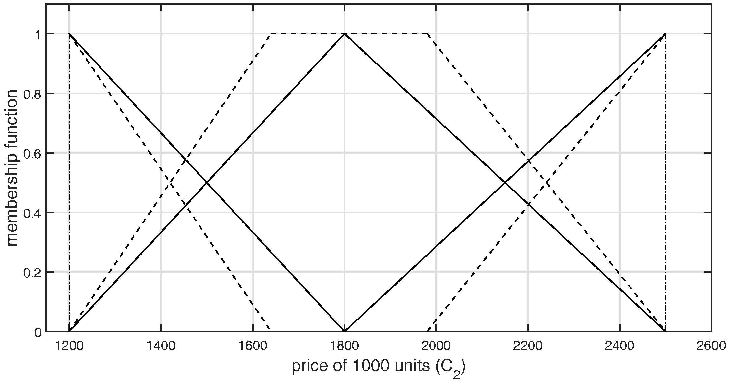
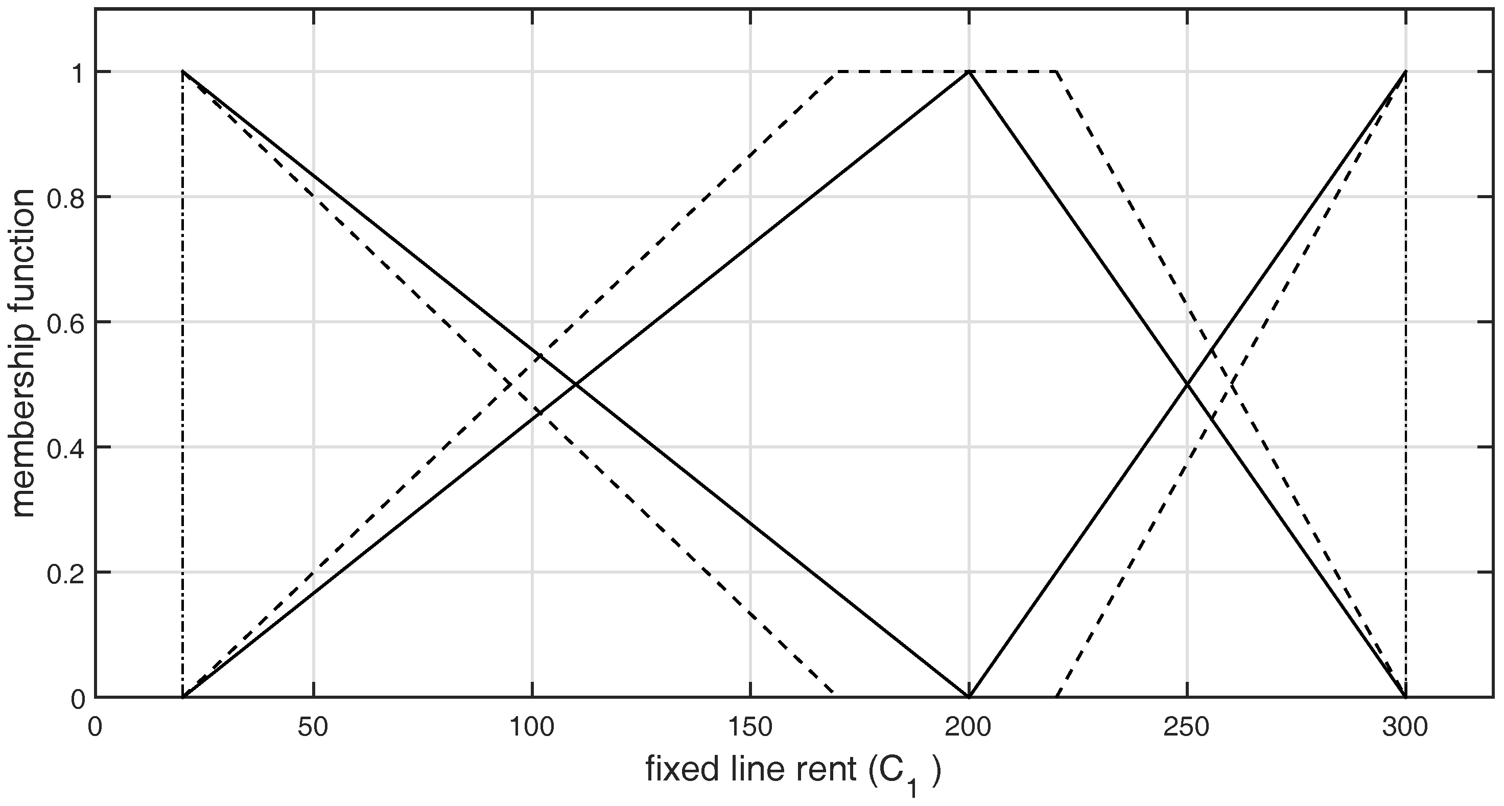
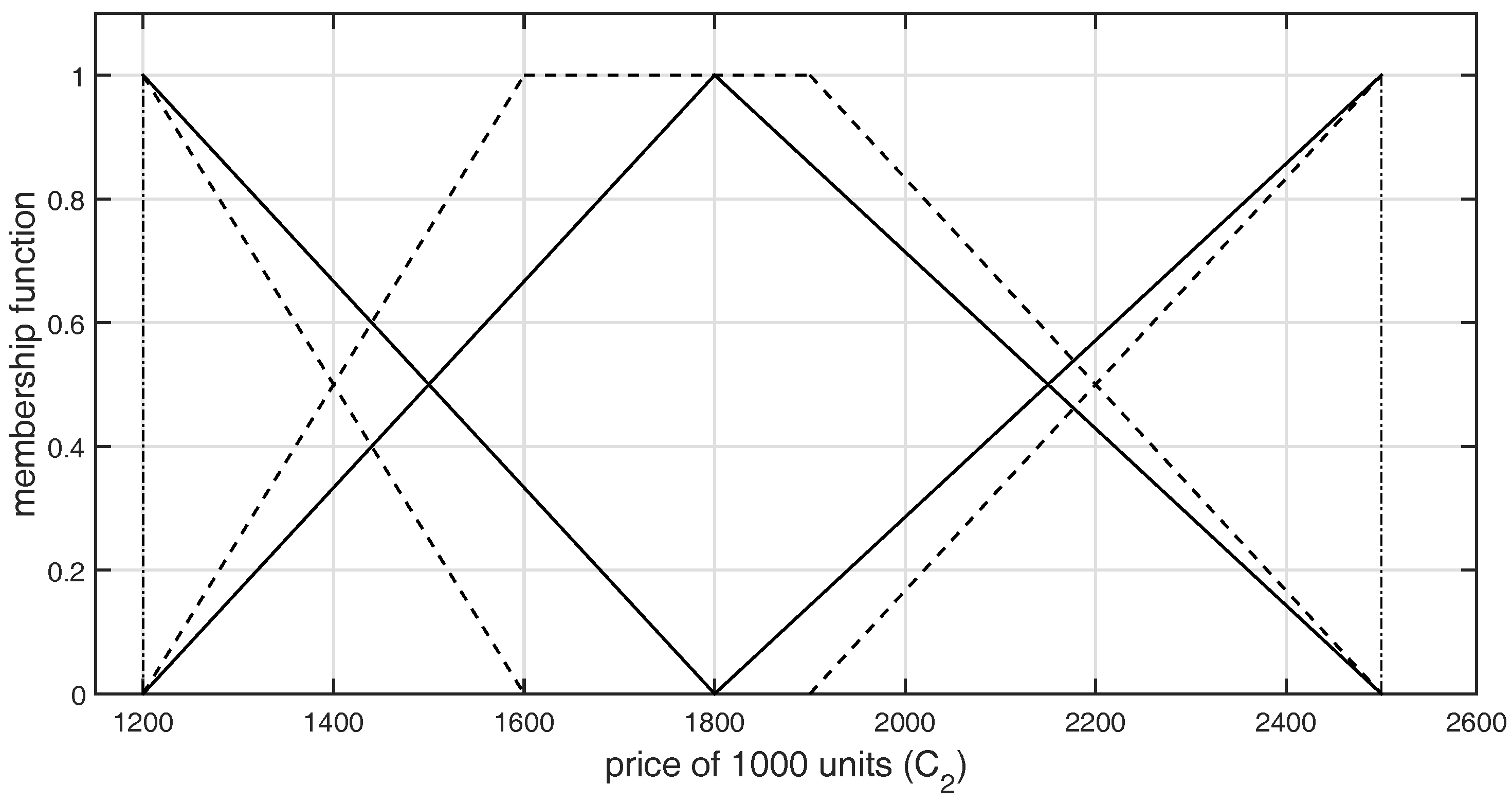
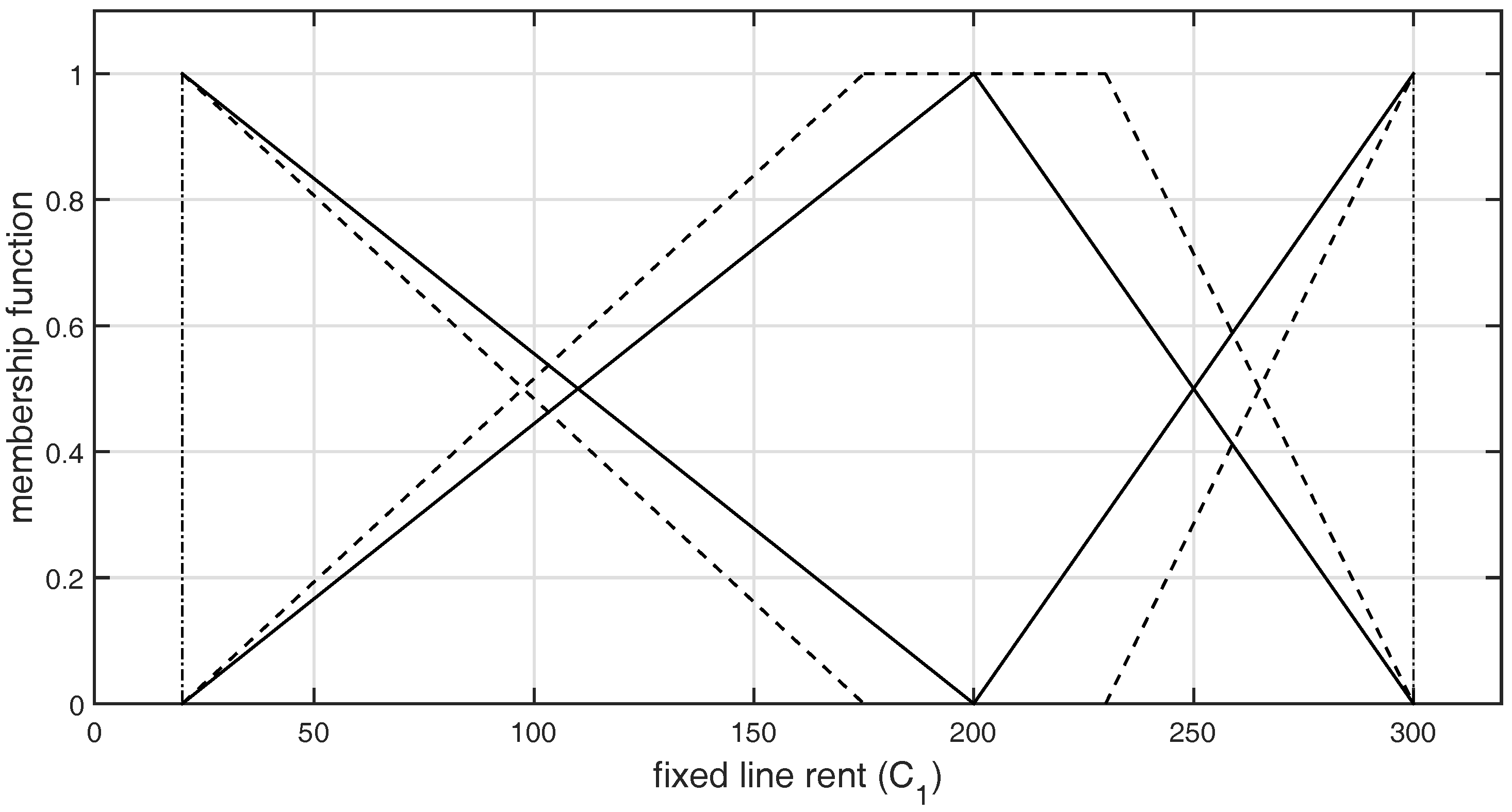
The graphical representation of L-R-type GFNs selected by the DMs for both the criteria and are shown in Figure 2, Figure 3, Figure 4, Figure 5, Figure 6 and Figure 7, respectively.
The cores of the family of TFNs for both the criteria and are respectively and The solution of the COMET is obtained for different number of COs. The simplest solution involves the use of nine COs, which are presented as follows:
To rank and evaluate the COs, suppose the three DMs give their assessments by providing the HFEs as shown in Table 5 and Table 6, and therefore, the Matrix of Expert Judgment (MEJ) is as follows:
The vector on the basis of is obtained as follows:
Each component of the vector represents the approximate values of the preference for the generated COs. Each CO and the value of preference is converted to a fuzzy rule, as follows:
With respect to Model 4, for the alternative , we have nine rules (COs), but the activated rules are The approximate values of the preference of corresponding COs are The HFE and the preference value of the corresponding alternative are computed respectively as follows:
Similarly, we can find the preference values for the rest of the alternatives and their ranking, which are shown in Table 7.
The best choice is the alternative followed by and . The worst choice is the alternative . The extrema elements are consistent with the original ranking. However, the ranking obtained by the COMET method is not perfect. The main reason is that this problem was solved under an uncertain environment by a group of decision-makers. In other words, it is extremely difficult to make a reliable decision using uncertain data, but we believe that it is possible. This example also illustrates how hard it is to make a group decision under uncertainty. Notwithstanding, the COMET method shows the best and the worst decision.
The main contribution of the proposed approach can be expressed by the most important properties of this extension, i.e., the proposed approach is completely free of the rank reversal phenomenon and obtains not only a discrete value of priority, but the mathematical function, which can be used to calculate the priority for all alternatives from the space of the problem. Quantitative expression of efficiency is a very difficult task because a large number of assumptions is needed. Additionally, the reference ranking of the alternatives set is needed in this task, but the reference rank is almost always unknown. However, the problem of quantitative effectiveness assessment is a very important and interesting direction for further research.
5. Conclusions
The hesitant fuzzy sets theory is a useful tool to deal with uncertainty in multi-criteria group decision-making problems. Various sources of uncertainty can be a challenge to make a reliable decision. The paper presented the extension of the COMET method, which was proposed for solving real-life problems under the opinions of experts in a hesitant fuzzy environment. Therefore, the proposed approach successfully helps to deal with group decision-making under uncertainty. The basic concept of the proposed method is based on the distance of alternatives from the nearest characteristic objects and their values of preference. The characteristic objects are obtained from the crisp values of all of the considered fuzzy numbers for each criterion. The proposed method is different from all of the previous techniques for MCGDM due to the fact that it uses hesitant fuzzy sets theory and the modification of the COMET method. The prominent feature of the proposed method is that it could provide a useful and flexible way to efficiently facilitate DMs under a hesitant fuzzy environment. The related calculations are simple and have a low computational complexity. Hence, it enriched and developed the theories and methods of MCGDM problems and also provided a new idea for solving MCGDM problems. Finally, a practical example was given to verify the developed approach and to demonstrate its practicality and effectiveness.
During the research, some possible areas of improvement of the proposed approach were identified. From a formal way, the COMET method can be extended over intuitionistic fuzzy sets, hesitant intuitionistic fuzzy sets, hesitant intuitionistic fuzzy linguistic term sets or other uncertain forms. Additionally, analysis and improvement of the accuracy of the presented extension of the COMET method should be performed. The future works may cover the practical usage of the proposed approach in the different decision-making domains.
Acknowledgments
The work was supported by the National Science Centre, Decision No. DEC-2016/23/N/HS4/01931, and by the Faculty of Computer Science and Information Technology, West Pomeranian University of Technology, Szczecin statutory funds.
Author Contributions
This paper is a result of common work of the authors in all aspects
Conflicts of Interest
The authors declare no conflict of interest
References
- Pedrycz, W.; Ekel, P.; Parreiras, R. Fuzzy Multicriteria Decision-Making: Models, Methods and Applications; John Wiley & Sons: Hoboken, NJ, USA, 2010. [Google Scholar]
- Yeh, T.M.; Pai, F.Y.; Liao, C.W. Using a hybrid MCDM methodology to identify critical factors in new product development. Neural Comput. Appl. 2014, 24, 957–971. [Google Scholar] [CrossRef]
- Xu, Z. On consistency of the weighted geometric mean complex judgement matrix in AHP. Eur. J. Oper. Res. 2000, 126, 683–687. [Google Scholar] [CrossRef]
- Lu, N.; Liang, L. Correlation Coefficients of Extended Hesitant Fuzzy Sets and Their Applications to Decision Making. Symmetry 2017, 9, 47. [Google Scholar] [CrossRef]
- Zhou, L.; Chen, H. A generalization of the power aggregation operators for linguistic environment and its application in group decision-making. Knowl. Based Syst. 2012, 26, 216–224. [Google Scholar] [CrossRef]
- Zhou, L.; Chen, H.; Liu, J. Generalized power aggregation operators and their applications in group decision-making. Comput. Ind. Eng. 2012, 62, 989–999. [Google Scholar] [CrossRef]
- Sengupta, A.; Pal, T.K. Fuzzy Preference Ordering of Interval Numbers in Decision Problems; Springer: Berlin, Germany, 2009. [Google Scholar]
- Fang, Z.; Ye, J. Multiple Attribute Group Decision-Making Method Based on Linguistic Neutrosophic Numbers. Symmetry 2017, 9, 111. [Google Scholar] [CrossRef]
- Gao, J.; Liu, H. Reference-Dependent Aggregation in Multi-AttributeGroup Decision-Making. Symmetry 2017, 9, 43. [Google Scholar] [CrossRef]
- Wang, Z.-L.; You, J.-X.; Liu, H.-C. Uncertain Quality Function Deployment Using a Hybrid Group Decision Making Model. Symmetry 2016, 8, 119. [Google Scholar] [CrossRef]
- You, X.; Chen, T.; Yang, Q. Approach to Multi-Criteria Group Decision-Making Problems Based on the Best-Worst-Method and ELECTRE Method. Symmetry 2016, 8, 95. [Google Scholar] [CrossRef]
- Zadeh, L.A. Fuzzy sets. Inf. Control 1965, 8, 338–353. [Google Scholar] [CrossRef]
- Gitinavard, H.; Mousavi, S.M.; Vahdani, B. Soft computing-based new interval-valued hesitant fuzzy multi-criteria group assessment method with last aggregation to industrial decision problems. Soft Comput. 2017, 21, 3247–3265. [Google Scholar] [CrossRef]
- Zadeh, L.A. The concept of a linguistic variable and its applications to approximate reasoning-Part I. Inf. Sci. 1975, 8, 199–249. [Google Scholar] [CrossRef]
- Herrera, F.; Herrera-Viedma, E.; Verdegay, J.L. A model of consensus in group decision-making under linguistic assessments. Fuzzy Sets Syst. 1996, 78, 73–87. [Google Scholar] [CrossRef]
- Xu, Z.S. A method based on linguistic aggregation operators for group decision-making with linguistic preference relations. Inf. Sci. 2004, 166, 19–30. [Google Scholar] [CrossRef]
- Xu, Z.S. Deviation measures of linguistic preference relations in group decision-making. Omega 2005, 33, 249–254. [Google Scholar] [CrossRef]
- Atanassov, K.T. Intuitionistic fuzzy sets. Fuzzy Sets Syst. 1986, 20, 87–96. [Google Scholar] [CrossRef]
- Liu, Z.Q.; Miyamoto, S. Soft Computing and Human-Centered Machines; Springer: Berlin, Germany, 2000; pp. 9–33. [Google Scholar]
- Yager, R.R. On the theory of bags. Int. J. Gen. Syst. 1986, 13, 23–37. [Google Scholar] [CrossRef]
- Ding, Z.; Wu, Y. An Improved Interval-Valued Hesitant Fuzzy Multi-Criteria Group Decision-Making Method and Applications. Math. Comput. Appl. 2016, 21, 22. [Google Scholar] [CrossRef]
- Wibowo, S.; Deng, H.; Xu, W. Evaluation of cloud services: A fuzzy multi-criteria group decision making method. Algorithms 2016, 9, 84. [Google Scholar] [CrossRef]
- Zhang, J.; Hegde, G.G.; Shang, J.; Qi, X. Evaluating Emergency Response Solutions for Sustainable Community Development by Using Fuzzy Multi-Criteria Group Decision Making Approaches: IVDHF-TOPSIS and IVDHF-VIKOR. Sustainability 2016, 8, 291. [Google Scholar] [CrossRef]
- Torra, V. Hesitant fuzzy sets. Int. J. Intell. Syst. 2010, 25, 529–539. [Google Scholar] [CrossRef]
- Jin, B. ELECTRE method for multiple attributes decision making problem with hesitant fuzzy information. J. Intell. Fuzzy Syst. 2015, 29, 463–468. [Google Scholar] [CrossRef]
- Zhang, N.; Wei, G. Extension of VIKOR method for decision making problem based on hesitant fuzzy set. Appl. Math. Model. 2013, 37, 4938–4947. [Google Scholar] [CrossRef]
- Peng, J.J.; Wang, J.Q.; Wu, X.H. Novel multi-criteria decision-making approaches based on hesitant fuzzy sets and prospect theory. Int. J. Inf. Technol. Decis. Mak. 2016, 15, 621–643. [Google Scholar] [CrossRef]
- Peng, X.; Yang, Y. Interval-valued hesitant fuzzy soft sets and their application in decision making. Fundam. Inform. 2015, 141, 71–93. [Google Scholar] [CrossRef]
- Yu, D. Hesitant fuzzy multi-criteria decision making methods based on Heronian mean. Technol. Econ. Dev. Econ. 2017, 23, 296–315. [Google Scholar] [CrossRef]
- Zhu, B.; Xu, Z. Extended hesitant fuzzy sets. Technol. Econ. Dev. Econ. 2016, 22, 100–121. [Google Scholar] [CrossRef]
- Wu, Y.; Xu, C.; Zhang, H.; Gao, J. Interval Generalized Ordered Weighted Utility Multiple Averaging Operators and Their Applications to Group Decision-Making. Symmetry 2017, 9, 103. [Google Scholar] [CrossRef]
- Yu, D.; Zhang, W.; Huang, G. Dual hesitant fuzzy aggregation operators. Technol. Econ. Dev. Econ. 2016, 22, 194–209. [Google Scholar] [CrossRef]
- Liu, J.; Sun, M. Generalized power average operator of hesitant fuzzy numbers and its application in multiple attribute decision-making. J. Comput. Inf. Syst. 2013, 9, 3051–3058. [Google Scholar]
- Xia, M.; Xu, Z.; Chen, N. Some hesitant fuzzy aggregation operators with their application in group decision-making. Group Decis. Negot. 2013, 22, 259–279. [Google Scholar] [CrossRef]
- Yu, D.; Wu, Y.; Zhou, W. Multi-criteria decision-making based on Choquet integral under hesitant fuzzy environment. J. Comput. Inf. Syst. 2011, 7, 4506–4513. [Google Scholar]
- Zhang, Z. Hesitant fuzzy power aggregation operators and their application to multiple attribute group decision-making. Inf. Sci. 2013, 234, 150–181. [Google Scholar] [CrossRef]
- Chen, N.; Xu, Z.; Xia, M. Interval-valued hesitant preference relations and their applications to group decision-making. Knowl. Based Syst. 2013, 37, 528–540. [Google Scholar] [CrossRef]
- Peng, D.H.; Wang, T.D.; Gao, C.Y.; Wang, H. Continuous hesitant fuzzy aggregation operators and their application to decision-making under interval-valued hesitant fuzzy setting. Sci. World J. 2014, 2014, 897304. [Google Scholar] [CrossRef] [PubMed]
- Peng, J.J.; Wang, J.Q.; Wang, J.; Chen, X.H. Multi-criteria decision-making approach with hesitant interval-valued intuitionistic fuzzy sets. Sci. World J. 2014, 2014, 868515. [Google Scholar] [CrossRef] [PubMed]
- Wei, G.; Zhao, X.; Lin, R. Some hesitant interval-valued fuzzy aggregation operators and their applications to multiple attribute decision-making. Knowl. Based Syst. 2013, 46, 43–53. [Google Scholar] [CrossRef]
- Beg, I.; Rashid, T. Hesitant 2-tuple linguistic information in multiple attributes group decision-making. J. Intell. Fuzzy Syst. 2016, 30, 143–150. [Google Scholar] [CrossRef]
- Rashid, T.; Husnine, S.M. Multi-criteria Group decision-making by Using Trapezoidal Valued Hesitant Fuzzy Sets. Sci. World J. 2014, 2014, 304834. [Google Scholar] [CrossRef] [PubMed]
- Yu, D. Triangular hesitant fuzzy set and its application to teaching quality evaluation. J. Inf. Comput. Sci. 2013, 10, 1925–1934. [Google Scholar] [CrossRef]
- Piegat, A.; Sałabun, W. Nonlinearity of human multi-criteria in decision-making. J. Theor. Appl. Comput. Sci. 2012, 6, 36–49. [Google Scholar]
- Sałabun, W. The Characteristic Objects Method, A new distance based approach to multi-criteria decision-making problems. J. Multi Criteria Decis. Anal. 2015, 22, 37–50. [Google Scholar] [CrossRef]
- Sałabun, W. The Characteristic Objects Method: A new approach to Identify a multi-criteria group decision-making problems. Int. J. Comput. Technol. Appl. 2014, 5, 1597–1602. [Google Scholar]
- Sałabun, W. Application of the fuzzy multi-criteria decision-making method to identify nonlinear decision models. Int. J. Comput. Appl. 2014, 89, 1–6. [Google Scholar] [CrossRef]
- Sałabun, W.; Piegat, A. Comparative analysis of MCDM methods for the assessment of mortality in patients with acute coronary syndrome. Artif. Intell. Rev. 2016, 1–15. [Google Scholar] [CrossRef]
- Faizi, S.; Rashid, T.; Sałabun, W.; Zafar, S.; Wątróbski, J. Decision Making with Uncertainty Using Hesitant Fuzzy Sets. Int. J. Fuzzy Syst. 2017, 1–11. [Google Scholar] [CrossRef]
- Piegat, A.; Sałabun, W. Identification of a multicriteria decision-making model using the characteristic objects method. Appl. Comput. Intell. Soft Comput. 2014, 2014, 1–14. [Google Scholar] [CrossRef]
- Sałabun, W.; Ziemba, P.; Wątróbski, J. The Rank Reversals Paradox in Management Decisions: The Comparison of the AHP and COMET Methods. In Intelligent Decision Technologies; Springer: Berlin, Germany, 2016; pp. 181–191. [Google Scholar]
- Wątróbski, J.; Jankowski, J. Guideline for MCDA method selection in production management area. In New Frontiers in Information and Production Systems Modelling and Analysis; Springer: Berlin, Germany, 2016; pp. 119–138. [Google Scholar]
- Sałabun, W.; Ziemba, P. Application of the Characteristic Objects Method in Supply Chain Management and Logistics. In Recent Developments in Intelligent Information and Database Systems; Springer: Berlin, Germany, 2016; pp. 445–453. [Google Scholar]
- Bector, C.R.; Chandra, S. Fuzzy mathematical programming and fuzzy matrix games; Springer: Berlin, Germany, 2005; Volume 169. [Google Scholar]
- Chakeri, A.; Dariani, A.N.; Lucas, C. How can fuzzy logic determine game equilibriums better? In Proceedings of the 4th International IEEE Conference Intelligent Systems, 2008 IS’08, Varna, Bulgaria, 6–8 September 2008; Volume 1, pp. 2–51. [Google Scholar]
- Chakeri, A.; Habibi, J.; Heshmat, Y. Fuzzy type-2 Nash equilibrium. In Proceedings of the 2008 International Conference on Computational Intelligence for Modelling Control & Automation, Vienna, Austria, 10–12 December 2008; pp. 398–402. [Google Scholar]
- Chakeri, A.; Sadati, N.; Dumont, G.A. Nash Equilibrium Strategies in Fuzzy Games. In Game Theory Relaunched; InTech: Exton, PA, USA, 2013. [Google Scholar]
- Chakeri, A.; Sadati, N.; Sharifian, S. Fuzzy Nash equilibrium in fuzzy games using ranking fuzzy numbers. In Proceedings of the 2010 IEEE International Conference on Fuzzy Systems (FUZZ), Barcelona, Spain, 18–23 July 2010; pp. 1–5. [Google Scholar]
- Chakeri, A.; Sheikholeslam, F. Fuzzy Nash equilibriums in crisp and fuzzy games. IEEE Trans. Fuzzy Syst. 2013, 21, 171–176. [Google Scholar] [CrossRef]
- Garagic, D.; Cruz, J.B. An approach to fuzzy noncooperative nash games. J. Optim. Theory Appl. 2003, 118, 475–491. [Google Scholar] [CrossRef]
- Sharifian, S.; Chakeri, A.; Sheikholeslam, F. Linguisitc representation of Nash equilibriums in fuzzy games. In Proceedings of the 2010 Annual Meeting of the North American Fuzzy Information Processing Society (NAFIPS), Toronto, ON, Canada, 12–14 July 2010; pp. 1–6. [Google Scholar]
- Sharma, R.; Gopal, M. Hybrid game strategy in fuzzy Markov-game-based control. IEEE Trans. Fuzzy Syst. 2008, 16, 1315–1327. [Google Scholar] [CrossRef]
- Tan, C.; Jiang, Z.Z.; Chen, X.; Ip, W.H. A Banzhaf function for a fuzzy game. IEEE Trans. Fuzzy Syst. 2014, 22, 1489–1502. [Google Scholar] [CrossRef]
- Piegat, A.; Sałabun, W. Comparative analysis of MCDM methods for assessing the severity of chronic liver disease. In Proceedings of the 14th International Conference on Artificial Intelligence and Soft Computing, Zakopane, Poland, 14–18 June 2015; pp. 228–238. [Google Scholar]
- Wątróbski, J.; Sałabun, W. The characteristic objects method: a new intelligent decision support tool for sustainable manufacturing. In Sustainable Design and Manufacturing; Springer: Berlin, Germany, 2016; pp. 349–359. [Google Scholar]
- Jankowski, J.; Sałabun, W.; Wątróbski, J. Identification of a multi-criteria assessment model of relation between editorial and commercial content in web systems. In Multimedia and Network Information Systems; Springer: Berlin, Germany, 2017; pp. 295–305. [Google Scholar]
- Velasquez, M.; Hester, P.T. An Analysis of Multi-Criteria Decision Making Methods. Int. J. Oper. Res. 2013, 10, 56–66. [Google Scholar]
- Xia, M.; Xu, Z. Hesitant fuzzy information aggregation in decision-making. Int. J. Approx. Reason. 2011, 52, 395–407. [Google Scholar] [CrossRef]
- Zimmermann, H.J. Fuzzy Set Theory—And Its Applications; Springer Science and Business Media: Berlin, Germany, 2001. [Google Scholar]
- Chen, J.; Huang, X. Dual Hesitant Fuzzy Probability. Symmetry 2017, 9, 52. [Google Scholar] [CrossRef]
- Liu, X.; Wang, Z.; Zhang, S. A Modification on the Hesitant Fuzzy Set Lexicographical Ranking Method. Symmetry 2016, 8, 153. [Google Scholar] [CrossRef]
- Zhang, X.; Xu, Z.; Liu, M. Hesitant trapezoidal fuzzy QUALIFLEX method and its application in the evaluation of green supply chain initiatives. Sustainability 2016, 8, 952. [Google Scholar] [CrossRef]
- Piegat, A. Fuzzy Modeling and Control; Springer: New York, NY, USA, 2001. [Google Scholar]
- Wang, G.; Wang, H. Non-fuzzy versions of fuzzy reasoning in classical logics. Inf. Sci. 2001, 138, 211–236. [Google Scholar] [CrossRef]
- Ross, T.J. Fuzzy Logic with Engineering Applications; John Wiley & Sons: Hoboken, NJ, USA, 2010. [Google Scholar]
- Klement, E.P.; Mesiar, R.; Pap, E. Triangular Norms; Kluwer Academic Publishers: Dordrecht, The Netherlands, 2000. [Google Scholar]
Figure 1.
The procedure of the proposed extension of COMET to group decision-making.
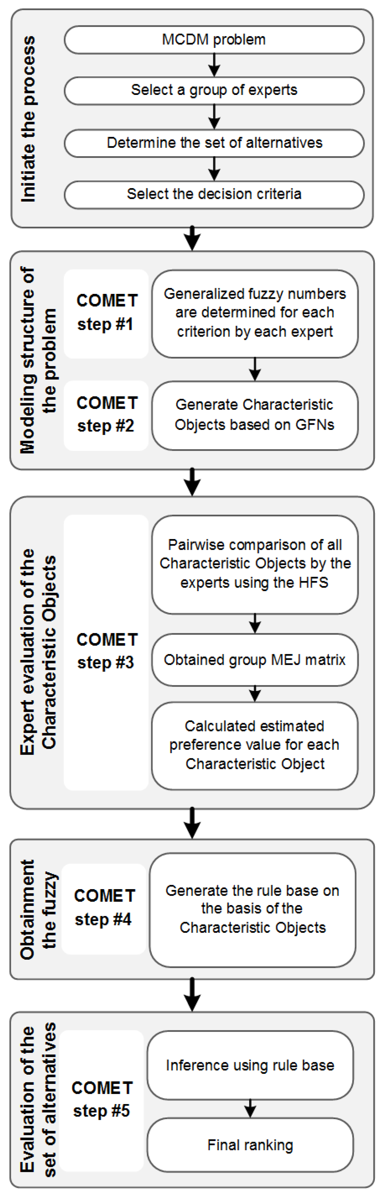
Figure 2.
Graphical representation of -type GFNs selected by DM1 for the criterion .

Figure 3.
Graphical representation of -type GFNs selected by DM1 for the criterion .

Figure 4.
Graphical representation of -type GFNs selected by DM2 for the criterion .

Figure 5.
Graphical representation of -type GFNs selected by DM2 for the criterion .
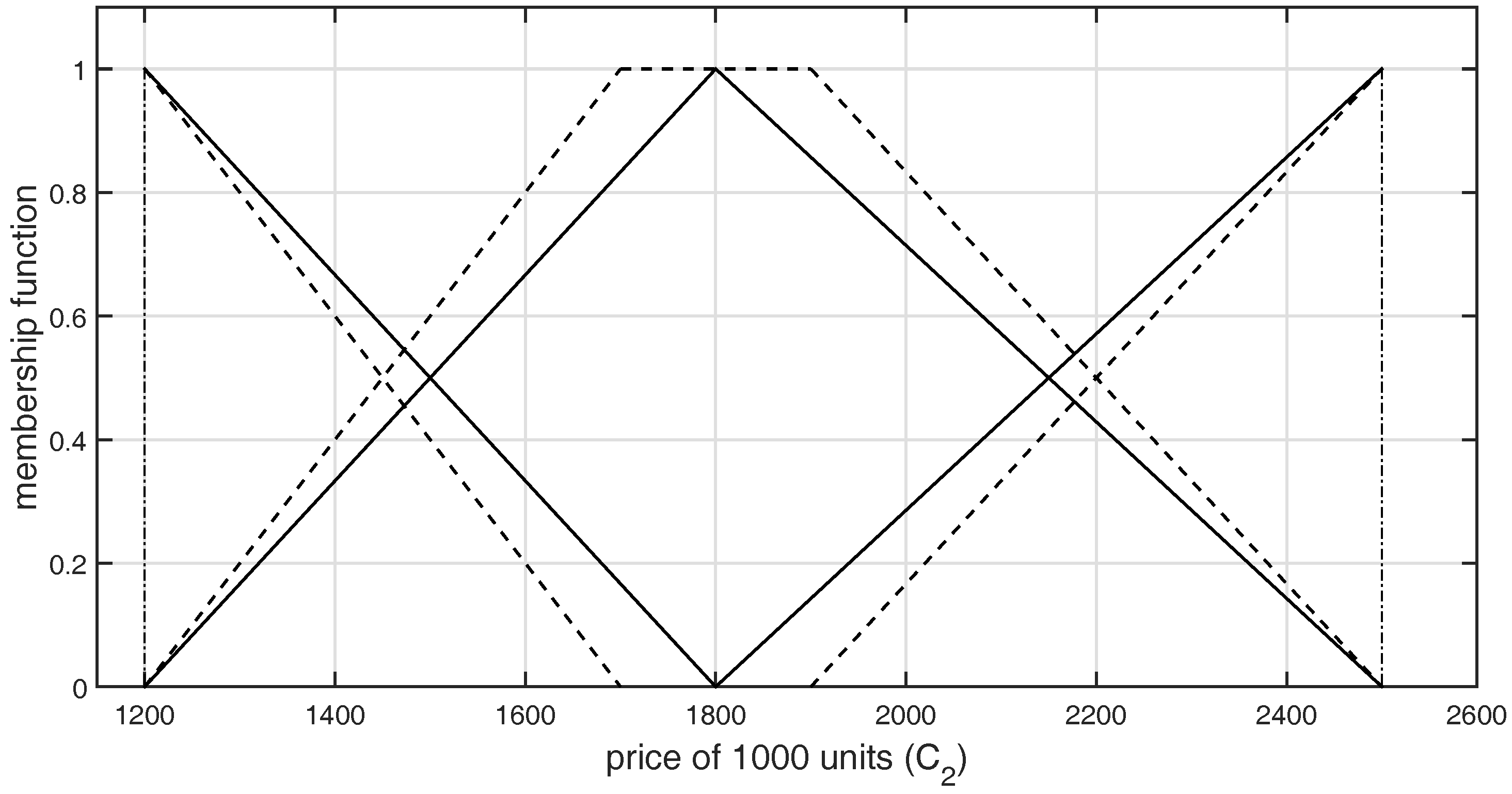
Figure 6.
Graphical representation of -type GFNs selected by DM3 for the criterion .
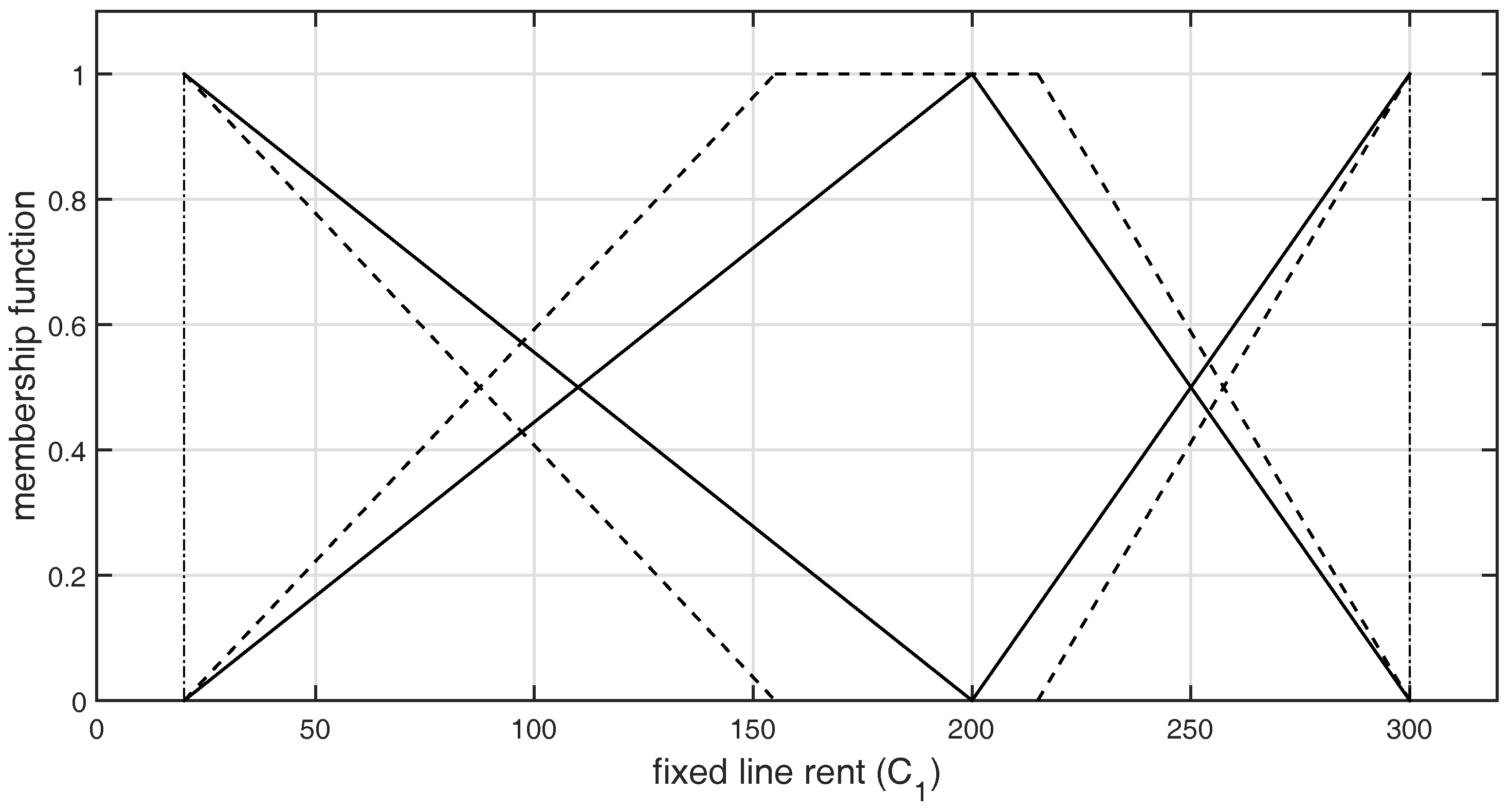
Figure 7.
Graphical representation of -type GFNs selected by DM3 for the criterion .

Table 1.
Original ranking of the alternatives, where LR - fixed line rent and R/U - rates per unit.
| Alternatives | (LR) | (R/U) | Bill Amount | Original Rank |
|---|---|---|---|---|
| 150 | 1500 | 1650 | 2 | |
| 50 | 2000 | 2050 | 3 | |
| 250 | 1250 | 1500 | 1 | |
| 30 | 2150 | 2180 | 4 |
Table 2.
LR-type Group Fuzzy Numbers (GFNs) selected by the Decision-Makers (DMs) for criteria .
| DM1 | |
| DM2 | |
| DM3 | |
Table 3.
LR-type GFNs selected by the DMs for criteria .
| DM1 | |
| DM2 | |
| DM3 | |
Table 4.
Average of the membership values obtained from LR-type GFNs for criteria .
| Average of the Membership Values Obtained from LR-Type GFNs for Criterion | |||
|---|---|---|---|
| 30 | 50 | 150 | 250 |
| 1250 | 1500 | 2000 | 2150 |
Table 5.
Matrix of Expert Judgment ().
Table 6.
Matrix of Expert Judgment ().
Table 7.
Comparison of the original ranking with the ranking obtained using the proposed method.
| Alternatives | (LR) | (R/U) | Original Ranking | Preference Values | New Ranking |
|---|---|---|---|---|---|
| 150 | 1500 | 2 | 3 | ||
| 50 | 2000 | 3 | 2 | ||
| 250 | 1250 | 1 | 1 | ||
| 30 | 2150 | 4 | 4 |
© 2017 by the authors. Licensee MDPI, Basel, Switzerland. This article is an open access article distributed under the terms and conditions of the Creative Commons Attribution (CC BY) license (http://creativecommons.org/licenses/by/4.0/).
Share and Cite
MDPI and ACS Style
Faizi, S.; Sałabun, W.; Rashid, T.; Wątróbski, J.; Zafar, S. Group Decision-Making for Hesitant Fuzzy Sets Based on Characteristic Objects Method. Symmetry 2017, 9, 136. https://doi.org/10.3390/sym9080136
AMA Style
Faizi S, Sałabun W, Rashid T, Wątróbski J, Zafar S. Group Decision-Making for Hesitant Fuzzy Sets Based on Characteristic Objects Method. Symmetry. 2017; 9(8):136. https://doi.org/10.3390/sym9080136
Chicago/Turabian StyleFaizi, Shahzad, Wojciech Sałabun, Tabasam Rashid, Jarosław Wątróbski, and Sohail Zafar. 2017. "Group Decision-Making for Hesitant Fuzzy Sets Based on Characteristic Objects Method" Symmetry 9, no. 8: 136. https://doi.org/10.3390/sym9080136
Note that from the first issue of 2016, this journal uses article numbers instead of page numbers. See further details here.