Hybrid Second-Order Iterative Algorithm for Orthogonal Projection onto a Parametric Surface


1
College of Data Science and Information Engineering, Guizhou Minzu University, Guiyang 550025, China
2
School of Mathematics and Computer Science, Yichun University, Yichun 336000, China
3
Center for Economic Research, Shandong University, Jinan 250100, China
4
Department of Science, Taiyuan Institute of Technology, Taiyuan 030008, China
5
Center for the World Ethnic Studies, Guizhou Minzu University, Guiyang 550025, China
*
Author to whom correspondence should be addressed.
†
These authors contributed equally to this work.
Symmetry 2017, 9(8), 146; https://doi.org/10.3390/sym9080146
Submission received: 15 June 2017
/
Revised: 21 July 2017
/
Accepted: 28 July 2017
/
Published: 5 August 2017
(This article belongs to the Special Issue Advances in Computer Graphics, Geometric Modeling, and Virtual and Augmented Reality)
Abstract
:To compute the minimum distance between a point and a parametric surface, three well-known first-order algorithms have been proposed by Hartmann (1999), Hoschek, et al. (1993) and Hu, et al. (2000) (hereafter, the First-Order method). In this paper, we prove the method’s first-order convergence and its independence of the initial value. We also give some numerical examples to illustrate its faster convergence than the existing methods. For some special cases where the First-Order method does not converge, we combine it with Newton’s second-order iterative method to present the hybrid second-order algorithm. Our method essentially exploits hybrid iteration, thus it performs very well with a second-order convergence, it is faster than the existing methods and it is independent of the initial value. Some numerical examples confirm our conclusion.
1. Introduction
In this paper, we discuss how to compute the minimum distance between a point and a parametric surface, and to return the nearest point (footpoint) on the surface as well as its corresponding parameter, which is also called the point projection problem (or the point inversion problem) of a parametric surface. It is a very interesting problem in geometric modeling, computer graphics and computer vision [1]. Both projection and inversion are essential for interactively selecting curves and surfaces [1,2], for the curve fitting problem [1,2], for reconstructing surfaces [3,4,5] and for projecting a space curve onto a surface for surface curve design [6,7]. It is also a key issue in the ICP (iterative closest point) algorithm for shape registration [8]. Mortenson (1985) [9] turns the projection problem into finding the root of a polynomial, then finds the root by using the Newton–Raphson method. Zhou et al. (1993) [10] present an algorithm for computation of the stationary points of the squared distance functions between two point sets. The problem is reformulated in terms of solution of n polynomial equations with n variables expressed in the tensor product Bernstein basis. Johnson and Cohen (2005) [11] present a robust search for distance extrema from a point to a curve or a surface. The robustness comes from using geometric operations with tangent cones rather than numerical methods to find all local extrema. Limaien and Trochu (1995) [12] compute the orthogonal projection of a point onto parametric curves and surfaces by constructing an auxiliary function and finding its zeros. Polak et al. (2003) [13] present a new feedback precision-adjustment rule with a smoothing technique and standard unconstrained minimization algorithms in the solution of finite minimax problems. Patrikalakis and Maekawa (2001) [14] reduce the distance function problem to solving systems of nonlinear polynomial equations. Based on Ma et al. [1], Selimovic (2006) [15] presents improved algorithms for the projection of points on NURBS curves and surfaces. Cohen et al. (1980) [16] provide classical subdivision algorithms which have been widely applied in computer-aided geometric design, computer graphics, and numerical analysis. Based on the subdividing concept [16], Piegl and Tiller (1995) [17] present an algorithm for point projection on NURBS surfaces by subdividing a NURBS surface into quadrilaterals, projecting the test point onto the closest quadrilateral, and then recover the parameter from the closest quadrilateral. Liu et al. (2009) [18] propose a local surface approximation technique—torus patch approximation—and prove that the approximation torus patch and the original surface are second-order osculating. By using the tangent line and the rectifying plane, Li et al. (2013) [19] present an algorithm for finding the intersection between the two spatial parametric curves. Hu et al. (2005) [8] use curvature iteration information for solving the projection problem. Scholars (Ku-Jin Kim (2003) [20], Li et al. (2004) [21], Chen et al. (2010) [22], Chen et al. (2009) [23], Bharath Ram Sundar et al. (2014) [24]) have fully analyzed and discussed the intersection curve between two surfaces, the minimum distance between two curves, the minimum distance between curve and surface and the minimum distance between two surfaces. By clipping circle technology, Chen et al. (2008) [25] provide a method for computing the minimum distance between a point and a NURBS curve. Then, based on clipping sphere strategy, Chen et al. (2009) [26] propose a method for computing the minimum distance between a point and a clamped B-spline surface. Being analogous to [25,26], based on an efficient culling technique that eliminates redundant curves and surfaces which obviously contain no projection from the given point, Young-Taek Oh et al. (2012) [27] present an efficient algorithm for projecting a given point to its closest point on a family of freeform curves and surfaces. Song et al. (2011) [7] propose an algorithm for calculating the orthogonal projection of parametric curves onto B-spline surfaces. It uses a second-order tracing method to construct a polyline to approximate the pre-image curve of the orthogonal projection curve in the parametric domain of the base surface. Regarding the projection problem, Kwanghee Ko et al. (2014) [28] give a detailed review on literatures before 2014. To sum up, those algorithms employ various techniques such as turning the problem into finding the root of the system of nonlinear equations, geometric methods, subdivision methods and circular clipping algorithms. It is well known that there are three classical first-order algorithms for computing the minimum distance between a point and a parametric surface [29,30,31]. However, they did not prove convergence for the First-Order method. In this paper, we contribute in two aspects. Firstly, we prove the method’s first-order convergence and its independence of the initial value. We also give some numerical examples to illustrate its faster convergence than the existing ones. Secondly, for some special cases where the First-Order method does not converge, we combine it with Newton’s second-order iterative method to present the hybrid second-order algorithm. Our method essentially exploits hybrid iteration, thus it performs very well with a second-order convergence, it is faster than the existing methods, and it is independent of the initial value. Some numerical examples confirm our conclusion.
The rest of this paper is organized as follows. Section 2 presents a convergence analysis for the First-Order method for orthogonal projection onto a parametric surface. In Section 3, some numerical examples illustrate that it converges faster than the existing methods. In Section 4, for some special cases where the First-Order method is not convergent, an improved hybrid second-order algorithm is presented. Convergence analysis and experimental results for the hybrid second-order algorithm are also presented in this section. Finally, Section 5 concludes the paper.
2. Convergence Analysis for the First-Order Method
In this section, we prove that the method defined by (5) is the first-order convergent and its convergence is independent of the initial value.
Assume a regular parametric surface , i.e., is a test point. The first-order geometric iteration [29,30,31] to compute the footpoint q of the test point p is the following. Projecting the test point p onto a tangent plane of the parametric surface at yields a point q determined by and the partial derivatives , . (see the following Formulas (2) and (3)). The footpoint can be approximatively expressed in the following way
where
Multiplying with and , respectively, we obtain
where denotes the scalar product of vectors , and denotes the norm of a vector x. The corresponding solution of a regular system of linear Equation (4) is
where , , , , .
We update by adding , and repeat the above procedure until and where is a given tolerance. This is the first-order geometric iteration method in [29,30,31] (See Figure 1). Furthermore, convergence of the First-Order method is independent of the initial value.
Theorem 1.
The method defined by (5) is the first-order convergent. Convergence of the iterative Formula (5) is independent of the initial value.
Proof.
We firstly derive the expression of footpoint q. Assume that parameter takes the value so that the test point orthogonally projects onto the parametric surface . It is not difficult to show that there is a relational expression
where and tangent vector , , = , . The relationship can also be expressed in the following way,
Because the footpoint q is the intersection of the tangent plane of the parametric surface at and the perpendicular line determined by test point p, the equation of the tangent plane of the parametric surface at is
At the same time, the vector of the line segment connected by the test point p and the point is
Because the vector (9) and the tangent vectors , , are orthogonal to each other, respectively, we naturally obtain a system of nonlinear equations of the parameters ,
So the corresponding solutions of parameters of the Formula (10) are
where
Substituting (11) into (8), and simplifying, we have
So the footpoint is the Formula (12). Substituting (12) into (5), and simplifying, we obtain the relationship,
where , , , , .
Using Taylor’s expansion, we obtain
where , ,,,,.
Thus, we have
and
From (7) and (14), then we have
By (14)–(16), and using Taylor’s expansion, Formula (13) can be transformed into the following form,
where
From (17), we can obtain and . So Formula (18) can be transformed into the following form
Using Taylor’s expansion by symbolic computation software Maple 18, and simplifying, we obtain
where ,, . Formula (20) can be further simplified into the following form,
where , .
The result of Formula (21) implies that the iterative Formula (5) is the first-order convergent. In the following, we continue to illustrate that convergence of the iterative Formula (5) is independent of the initial value(See Figure 2).
Our proof method is analogous to those methods in references [32,33]. We project all points, curves and the surface of Figure 1 onto the plane, and this yields Figure 2. When the iterative Formula (5) starts to iterate, according to the graphical demonstration, the corresponding parametric value of the footpoint q is . The middle point of point and point is M where . From the graphic demonstration, there are two inequality relationships and . These results indicate two inequality relationships and ; namely, there is an iterative relational error expression , where . To sum up, we can verify that convergence of the iterative Formula (5) is independent of the initial value. ☐
3. Numerical Examples
Example 1.
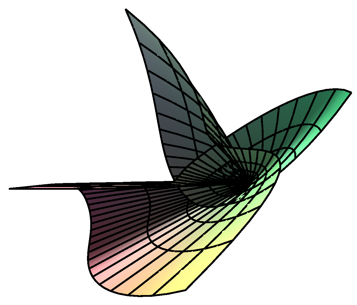
There is a general parametric surface = , cos, sin, with a test point . Using the First-Order method, the corresponding orthogonal projection parametric value is =, the initial iterative values are , respectively. Each initial iterative value repeatedly iterates 10 times, respectively, yielding 10 different iteration times in the time unit of nanoseconds. In Table 1, the mean running time of the first-order iterative method is 134,760, 141,798, 41,033, 140,051, 137,059, and 42,399 nanoseconds for six different initial iterative values, respectively. In the end, the overall average running time in Table 1 is 106183.33 nanoseconds (≈0.10618 ms), while the overall average running time of Table 1 and Table 2 in [18] is 0.3565 ms. So the First-Order method is faster than the algorithm in [18]. (See Figure 3).
Example 2.
There is a quasi-B-spline parametric surface , =, with a test point . Using the First-Order method, the corresponding orthogonal projection parametric value is =, the initial iterative values are , respectively. Each initial iterative value repeatedly iterates 10 times, respectively, yielding 10 different iteration times in nanoseconds. In Table 2, the mean running time of the First-Order method is 500,831, 440,815, 480,969, 445,755, 426,737, and 488,092 nanoseconds for six different initial iterative values, respectively. In the end, the overall average running time is 463,866.50 nanoseconds (≈0.463865 ms), while the overall average running time of the Example 2 for the algorithm in [18] is 1.705624977 ms under the same initial iteration condition. So the First-Order method is faster than the algorithm in [18]. (See Figure 4).
In Table 1 and Table 2, the convergence tolerance required such that is displayed. The approximate zero found up to the 17th decimal place is displayed. All computations were done under g++ in Fedora linux 8 environment using our personal computer with T2080 1.73 GHz CPU and 2.5 GB memory. The overall average running time of 0.336222 ms in Examples 1 and 2 for their algorithm [18] means the First-Order method is faster than the algorithm in [18]. In [18], authors point out that their algorithm is faster than that in [8], which means the First-Order method is faster than the one in [8]. At the same time, the overall average running time of 61.81167 ms in three Examples for their algorithm [26] is obtained, then the First-Order method is faster than the algorithm in [26]. However, in [26], the authors indicate that their algorithm is faster than those in [1,15], which means the First-Order method is faster than the one in [1,15]. To sum up, the First-Order method converges faster than the existing methods in [1,8,15,18,26].
4. The Improved Algorithm
4.1. Counterexamples
In Section 2 and Section 3, convergence of the First-Order method is independent of the initial value and some numerical examples illustrate that it converges faster than the existing methods. To show some special cases where the First-Order method is not convergent, we create five counterexamples as follows.
Counterexample 1.
Suppose the parametric surface with a test point . It is clear that the uniquely corresponding orthogonal projection point and parametric value of the test point p are and , respectively. For any initial iterative value, the First-Order method could not converge to (0,0).
Counterexample 2.
Suppose a parametric surface with a test point . It is not difficult to know that the uniquely corresponding orthogonal projection point and parametric value of the test point p are , , and , respectively. Whatever initial iterative value is given, the First-Order method could not converge to , . In addition, for a parametric surface , for any test point p and any initial iterative value, the First-Order method could not converge.
Counterexample 3.
Suppose a parametric surface with a test point . It is easy to know that the uniquely corresponding orthogonal projection point and parametric value of the test point p are , and ,, respectively. For any initial iterative value, the First-Order iterative method could not converge to , . In ddition, for a parametric surface , for any test point p and any initial iterative value, the First-Order method could not converge.
Counterexample 4.
Suppose a parametric surface with a test point . It is known that the uniquely corresponding orthogonal projection point and parametric value of the test point p are and , respectively. For any initial iterative value, the First-order method could not converge to , . Furthermore, for a parametric surface , for any test point p and any initial iterative value, the First-Order method could not converge.
Counterexample 5.
Suppose a parametric surface with a test point . It is known that the uniquely corresponding orthogonal projection point and parametric value of the test point p are (1.0719814278710903,1.3399767848388629,−0.98067565161631654) and = (1.0719814278710903, 1.3399767848388629), respectively. For any initial iterative value, the First-Order method could not converge to (1.0719814278710903, 1.3399767848388629). Furthermore, for a parametric surface , for any test point p and any initial iterative value, the First-Order method could not converge.
4.2. The Improved Algorithm
Since the First-Order method is not convergent for some special cases, we present the improved algorithm which will converge for any parametric surface, test point and initial iterative value. For simplicity, we briefly write as t, namely, , . It is well known that the classic iterative method to solve a system of nonlinear equations is Newton’s method, whose iterative expression is
where the system is expressed as follows:
Then, the more specific expression of Newton’s iterative Formula (22) is the following,
where ,
. This method is quadratically convergent in a neighborhood of the solution where the Jacobian matrix is non-singular. Its convergence rate is greater than that of the First-Order method. However, a limitation of this method is that its convergence depends on the choice of the initial value. Only if the convergence condition for Newton’s second-order iterative method is satisfied, is the method effective. In order to improve the robustness of convergence, based on the First-Order convergence method, we present Algorithm 1 (the hybrid second-order algorithm) for orthogonal projection onto the parametric surface. The hybrid second-order algorithm essentially combines the respective advantages of these two methods: if the iterative parametric value from the First-Order geometric iteration method satisfies the convergence condition for Newton’s second-order iterative method, we then turn to the method to accelerate the convergence process. If not, we continue the First-Order geometric iteration method until its iterative parametric value satisfies the convergence condition for Newton’s second-order iterative method, and we then turn to it as above. Then comes the end of the whole algorithm. The procedure that we proposed guarantees that the whole iterative process is convergent, and its convergence is independent of the choice of the initial value. In addition, the procedure can increase its rapidity. The hybrid second-order iterative algorithm for computing the minimum distance between a point and a parametric surface can be realized as follows.
| Algorithm 1: The hybrid second-order algorithm. |
| Input: Input the initial iterative parametric value , parametric surface and test point p. |
| Output: Output the final iterative parametric value. |
|
| . |
| If |
| { |
| Using Newton’s second-order iterative Formula (22), compute |
| until the norm of difference between the former and |
| the latter is near 0(), then end this algorithm. |
| } |
| Else { |
| go to Step 2. |
| } |
Remark 1.
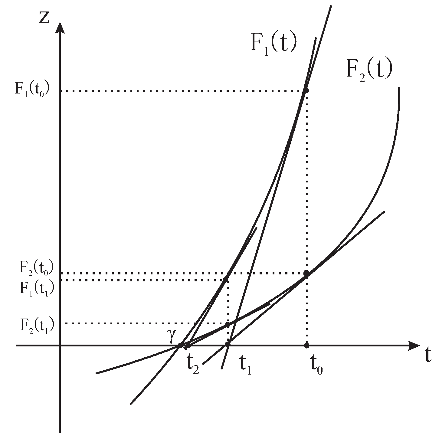
We give a geometric interpretation of Newton’s iterative method with two variables in Figure 5, where abscissa axis t represents the two-dimensional coordinate , the vertical coordinate z represents function value or . Curve and actually denote two surfaces in three-dimensional space, which are determined by the first and the second Formula in Equation (23), respectively. γ is the intersection point of two lines, the first of which is the intersection line of and plane t, and the second of which is the intersection line of and plane t. In another way, γ is the solution to Equation (23). Through point , draw a line perpendicular to the plane t, and then the perpendicular line intersects the surface and , respectively. The intersection points are designated as the first and the second intersection point, respectively. Through the first and the second intersection point, we make two tangent planes, respectively. These two tangent planes intersect with plane t and generate two intersection lines, which are designated as the first and the second intersection lines. Two intersection lines intersect to obtain the point . Given the intersection point , we repeat the procedure above to obtain the new first and the second intersection point, and then the new first and the second intersection lines. Finally, we can obtain the new intersection point . Repeat the above steps until the iterative value converges to =. Of course, it must satisfy the condition for the fixed point theorem of Newton’s iterative method before Newton’s iterative method starts to work.
Remark 2.
For some special cases, in Section 4, where the First-Order method is not convergent, our hybrid second-order algorithm could converge. In addition, we find that the method is convergent for any initial iterative value, any test point and parametric surface in many tested examples.
4.3. Convergence Analysis for the Improved Algorithm
Definition 1.
In Reference [34] (Fixed Point), a function G from into has a fixed point at if .
Theorem 2.
In Reference [34] (Fixed Point Theorem), let , for some collection of constants and . Suppose G is a continuous function from into with the property that whenever . Then, G has a fixed point in D. Moreover, suppose that all the component functions of G have continuous partial derivatives and a constant exists with , whenever , for each and each component function . Then, these sequence defined by an arbitrarily selected in D and generated by
This converges to the unique fixed point and satisfies the iterative relationship
In the following, we directly present the fixed point theorem for Newton’s iterative method.
Theorem 3.
Let for some collection of constants and . Suppose G (see Equation (24)) is a continuous function from into with the property that whenever . Then, G has a fixed point in D. Moreover, suppose that all the component functions of G have continuous partial derivatives and a constant exists with , whenever , for each and each component function . Then, these sequence defined by an arbitrarily selected in D and generated by
This converges to the unique fixed point and satisfies the iterative relationship
Theorem 4.
The convergence order of the hybrid second-order algorithm for orthogonal projection onto the parametric surface is 2. Convergence of the hybrid second-order algorithm is independent of the initial value.
Proof.
Let be a root of system , , where the system is expressed by Formula (23). Define and use Taylor’s expansion around , we have
Since is a simple zero of the Formula (23), so . Then, we have
where .
Using (21), and (29)–(31), we obtain
The result means that the hybrid algorithm is second-order convergent. According to the procedure of the hybrid second-order algorithm, if the iterative parametric value satisfies the convergence condition for Newton’s second-order iterative method, we then turn to Newton’s second-order iterative method. If not, we continue the First-Order geometric iteration method until its iterative parametric value satisfies the convergence condition of Newton’s second-order iterative method. Then comes the end of the whole algorithm. When the hybrid second-order iterative algorithm implements the First-Order iterative method, its independence of the initial value can be guaranteed by Theorem 1. When the hybrid second-order iterative algorithm implements Newton’s second-order iterative method, its independence of the initial value can be guaranteed by Theorem 3. To sum up, convergence of the hybrid second-order iterative algorithm is independent of the initial value throughout the whole algorithm operating process. ☐
4.4. Numerical Experiments
Example 3.
We replicate Example 1 using the hybrid second-order algorithm in Table 3 and compare it with results in Table 1. In Table 3, the mean running time of the hybrid second-order algorithm is 303,210.7, 319,045.5, 92,325.2, 315,116.9, 308,383.9, and 95,399.5 nanoseconds for six different initial iterative values, respectively. In the end, the overall average running time in Table 3 is 238,913.62 nanoseconds (≈0.2389 ms), while the overall average running time of Table 1 and Table 2 in [18] is 0.3565 ms. So our hybrid second-order algorithm is faster than the algorithm in [18]. On the other hand, from Table 3,
Example 4.
We replicate Example 2 using the hybrid second-order algorithm in Table 4 and compare it with results in Table 2. In Table 4, the mean running time of the hybrid second-order algorithm is 1,126,871, 991,834.4, 1,082,181, 1,002,949, 960,158.4, and 1,098,208 nanoseconds for six different initial iterative values, respectively. In the end, the overall average running time is 1,043,700 nanoseconds(≈1.0437 ms), while the overall average running time of the Example 2 for the algorithm in [18] is 1.705624977 ms under the same initial iteration condition. So the hybrid second-order algorithm is faster than the algorithm proposed in [18]. On the other hand, from Table 4,
In Table 3 and Table 4, the convergence tolerance, the decimal place of approximate zero and the computation environment are set as those in Table 1 and Table 2. The overall average running time of 0.336222 ms in Examples 3 and 4 for the algorithm in [18] implies that our hybrid second-order algorithm is faster than the algorithm in [18] . In [18], the authors point out that their algorithm is faster than the algorithm in [8], which means the hybrid second-order algorithm is faster than the one in [8]. At the same time, the overall average running time of 61.81167 ms in three Examples for their algorithm implies that our hybrid second-order algorithm is faster than the algorithm in [26]. However, in [26], the authors indicate that their algorithm is faster than the ones in [1,15], which means our hybrid second-order algorithm is faster than the ones in [1,15]. To sum up, with the exception of the First-Order method, our hybrid second-order algorithm converges faster than the existing methods in [1,8,15,18,26]. In Table 3 and Table 4, the unit of time is nanoseconds.
Remark 3.
The hybrid second-order algorithm presented can be applied for one projection point case for orthogonal projection of a test point onto a parametric surface . For the multiple orthogonal projection points situation, the basic idea of our approach is as follows:
- (1)
- Divide a parametric region of a parametric surface into sub-regions , where .
- (2)
- Randomly select an initial iterative parametric value in each sub-region.
- (3)
- For each initial iterative parametric value, holding other initial iterative parametric values fixed, use the hybrid second-order iterative algorithm and iterate until it converges. Let us assume that the converged iterative parametric values are , respectively.
- (4)
- Compute the local minimum distances , where .
- (5)
- Compute the global minimum distance . If we try to find all solutions as soon as possible, divide a parametric region of parametric surface into sub-regions , where such that M is very large.
Remark 4.
In addition to two test examples, we have also tested many other examples. According to these test results, for different initial iterative values, it can converge to the corresponding orthogonal projection point by using the hybrid second-order algorithm. Namely, if the initial iterative value is , which belongs to the parametric region of a parametric surface , the corresponding orthogonal projection parametric value for the test point is , and then the test point p and its corresponding orthogonal projection parametric value satisfy two inequality relationships
This indicates that these two inequality relationships satisfy Formula (6) or (7). Thus, it illustrates that convergence of the hybrid second-order algorithm is independent of the initial value. Furthermore, the hybrid second-order algorithm is robust and efficient as shown by the previous two of ten challenges proposed by [35].
5. Conclusions
This paper investigates the problem related to a point projection onto a parametric surface. To compute the minimum distance between a point and a parametric surface, three well-known first-order algorithms have been proposed by [29,30,31] (hereafter, the First-Order method). In this paper, we prove the method’s first-order convergence and its independence of the initial value. We also give some numerical examples to illustrate its faster convergence than the existing ones. For some special cases where the First-Order method does not converge, we combine it with Newton’s second-order iterative method to present the hybrid second-order algorithm. Our method essentially exploits hybrid iteration, thus it performs very well with a second-order convergence, it is faster than the existing methods and it is independent of the initial value. Some numerical examples confirm our conclusion. An area for future research is to develop a method for computing the minimum distance between a point and a higher-dimensional parametric surface.
Acknowledgments
We take the opportunity to thank anonymous reviewers for their thoughtful and meaningful comments. This work is supported by the National Natural Science Foundation of China (Grant No. 61263034), Scientific and Technology Foundation Funded Project of Guizhou Province (Grant No. [2014]2092, Grant No. [2014]2093), Feature Key Laboratory for Regular Institutions of Higher Education of Guizhou Province(Grant No. [2016]003), National Bureau of Statistics Foundation Funded Project (Grant No. 2014LY011), Key Laboratory of Pattern Recognition and Intelligent System of Construction Project of Guizhou Province (Grant No. [2009]4002), Information Processing and Pattern Recognition for Graduate Education Innovation Base of Guizhou Province. Linke Hou is supported by Shandong Provincial Natural Science Foundation of China(Grant No. ZR2016GM24). Juan Liang is supported by Scientific and Technology Key Foundation of Taiyuan Institute of Technology(Grant No. 2016LZ02). Qiaoyang Li is supported by Fund of National Social Science(No. 14XMZ001) and Fund of Chinese Ministry of Education(No. 15JZD034).
Author Contributions
The contributions of all of the authors are the same. All of them have worked together to develop the present manuscript.
Conflicts of Interest
The authors declare no conflict of interest.
References
- Ma, Y.L.; Hewitt, W.T. Point inversion and projection for NURBS curve and surface: Control polygon approach. Comput. Aided Geom. Des. 2003, 20, 79–99. [Google Scholar] [CrossRef]
- Yang, H.P.; Wang, W.P.; Sun, J.G. Control point adjustment for B-spline curve approximation. Comput. Aided Des. 2004, 36, 639–652. [Google Scholar] [CrossRef] [Green Version]
- Johnson, D.E.; Cohen, E. A Framework for efficient minimum distance computations. In Proceedings of the IEEE Intemational Conference on Robotics & Automation, Leuven, Belgium, 20 May 1998. [Google Scholar]
- Piegl, L.; Tiller, W. Parametrization for surface fitting in reverse engineering. Comput. Aided Des. 2001, 33, 593–603. [Google Scholar] [CrossRef]
- Pegna, J.; Wolter, F.E. Surface curve design by orthogonal projection of space curves onto free-form surfaces. ASME Trans. J. Mech. Design 1996, 118, 45–52. [Google Scholar] [CrossRef]
- Besl, P.J.; McKay, N.D. A method for registration of 3-D shapes. IEEE Trans. Pattern Anal. Mach. Intell. 1992, 14, 239–256. [Google Scholar] [CrossRef]
- Song, H.-C.; Yong, J.-H.; Yang, Y.-J.; Liu, X.-M. Algorithm for orthogonal projection of parametric curves onto B-spline surfaces. Comput.-Aided Des. 2011, 43, 381–393. [Google Scholar] [CrossRef]
- Hu, S.M.; Wallner, J. A second order algorithm for orthogonal projection onto curves and surfaces. Comput. Aided Geom. Des. 2005, 22, 251–260. [Google Scholar] [CrossRef]
- Mortenson, M.E. Geometric Modeling; Wiley: New York, NY, USA, 1985. [Google Scholar]
- Zhou, J.M.; Sherbrooke, E.C.; Patrikalakis, N. Computation of stationary points of distance functions. Eng. Comput. 1993, 9, 231–246. [Google Scholar] [CrossRef]
- Johnson, D.E.; Cohen, E. Distance extrema for spline models using tangent cones. In Proceedings of the 2005 Conference on Graphics Interface, Victoria, BC, Canada, 9–11 May 2005. [Google Scholar]
- Limaien, A.; Trochu, F. Geometric algorithms for the intersection of curves and surfaces. Comput. Graph. 1995, 19, 391–403. [Google Scholar] [CrossRef]
- Polak, E.; Royset, J.O. Algorithms with adaptive smoothing for finite minimax problems. J. Optim. Theory Appl. 2003, 119, 459–484. [Google Scholar] [CrossRef]
- Patrikalakis, N.; Maekawa, T. Shape Interrogation for Computer Aided Design and Manufacturing; Springer: Berlin, Germany, 2001. [Google Scholar]
- Selimovic, I. Improved algorithms for the projection of points on NURBS curves and surfaces. Comput. Aided Geom. Des. 2006, 23, 439–445. [Google Scholar] [CrossRef]
- Cohen, E.; Lyche, T.; Riesebfeld, R. Discrete B-splines and subdivision techniques in computer-aided geometric design and computer graphics. Comput. Graph. Image Proc. 1980, 14, 87–111. [Google Scholar] [CrossRef]
- Piegl, L.; Tiller, W. The NURBS Book; Springer: New York, NY, USA, 1995. [Google Scholar]
- Liu, X.-M.; Yang, L.; Yong, J.-H.; Gu, H.-J.; Sun, J.-G. A torus patch approximation approach for point projection on surfaces. Comput. Aided Geom. Des. 2009, 26, 593–598. [Google Scholar] [CrossRef]
- Li, X.W.; Xin, Q.; Wu, Z.N.; Zhang, M.S.; Zhang, Q. A geometric strategy for computing intersections of two spatial parametric curves. Vis. Comput. 2013, 29, 1151–1158. [Google Scholar] [CrossRef]
- Kim, K.-J. Minimum distance between a canal surface and a simple surface. Comput.-Aided Des. 2003, 35, 871–879. [Google Scholar] [CrossRef]
- Li, X.Y.; Jiang, H.; Chen, S.; Wang, X.C. An efficient surface-surface intersection algorithm based on geometry characteristics. Comput. Graph. 2004, 28, 527–537. [Google Scholar] [CrossRef]
- Chen, X.-D.; Ma, W.Y.; Xu, G.; Paul, J.-C. Computing the Hausdorff distance between two B-spline curves. Comput.-Aided Des. 2010, 42, 1197–1206. [Google Scholar] [CrossRef]
- Chen, X.-D.; Chen, L.Q.; Wang, Y.G.; Xu, G.; Yong, J.-H.; Paul, J.-C. Computing the minimum distance between two Bézier curves. J. Comput. Appl. Math. 2009, 229, 294–301. [Google Scholar] [CrossRef] [Green Version]
- Sundar, B.R.; Chunduru, A.; Tiwari, R.; Gupta, A.; Muthuganapathy, R. Footpoint distance as a measure of distance computation between curves and surfaces. Comput. Graph. 2014, 38, 300–309. [Google Scholar] [CrossRef]
- Chen, X.-D.; Yong, J.-H.; Wang, G.Z.; Paul, J.-C.; Xu, G. Computing the minimum distance between a point and a NURBS curve. Comput.-Aided Des. 2008, 40, 1051–1054. [Google Scholar] [CrossRef] [Green Version]
- Chen, X.-D.; Xu, G.; Yong, J.-H.; Wang, G.Z.; Paul, J.-C. Computing the minimum distance between a point and a clamped B-spline surface. Graph. Model. 2009, 71, 107–112. [Google Scholar] [CrossRef] [Green Version]
- Oh, Y.-T.; Kim, Y.-J.; Lee, J.; Kim, Y.-S.; Elber, G. Efficient point-projection to freeform curves and surfaces. Comput. Aided Geom. Des. 2012, 29, 242–254. [Google Scholar] [CrossRef]
- Ko, K.; Sakkalis, T. Orthogonal projection of points in CAD/CAM applications: An overview. J. Comput. Des. Eng. 2014, 1, 116–127. [Google Scholar] [CrossRef]
- Hartmann, E. On the curvature of curves and surfaces defined by normal forms. Comput. Aided Geom. Des. 1999, 16, 355–376. [Google Scholar] [CrossRef]
- Hoschek, J.; Lasser, D. Fundamentals of Computer Aided Geometric Design; A.K. Peters, Ltd.: Natick, MA, USA, 1993. [Google Scholar]
- Hu, S.M.; Sun, J.G.; Jin, T.G.; Wang, G.Z. Computing the parameter of points on NURBS curves and surfaces via moving affine frame method. J. Softw. 2000, 11, 49–53. (In Chinese) [Google Scholar]
- Melmant, A. Geometry and convergence of eulers and halleys methods. SIAM Rev. 1997, 39, 728–735. [Google Scholar] [CrossRef]
- Traub, J.F. A Class of globally convergent iteration functions for the solution of polynomial equations. Math. Comput. 1966, 20, 113–138. [Google Scholar] [CrossRef]
- Burden, R.L.; Faires, J.D. Numerical Analysis, 9th ed.; Brooks/Cole Cengage Learning: Boston, MA, USA, 2011. [Google Scholar]
- Piegl, L.A. Ten challenges in computer-aided design. Comput.-Aided Des. 2005, 37, 461–470. [Google Scholar] [CrossRef]
Figure 1.
Graphic demonstration of the First-Order method.
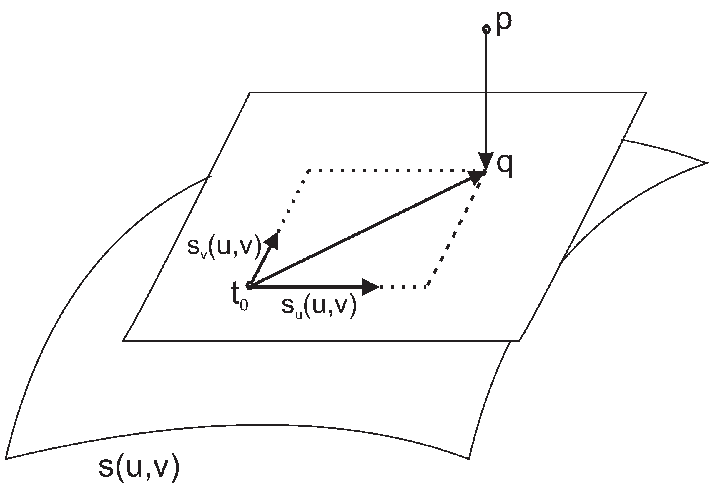
Figure 2.
Graphic demonstration for convergence analysis.
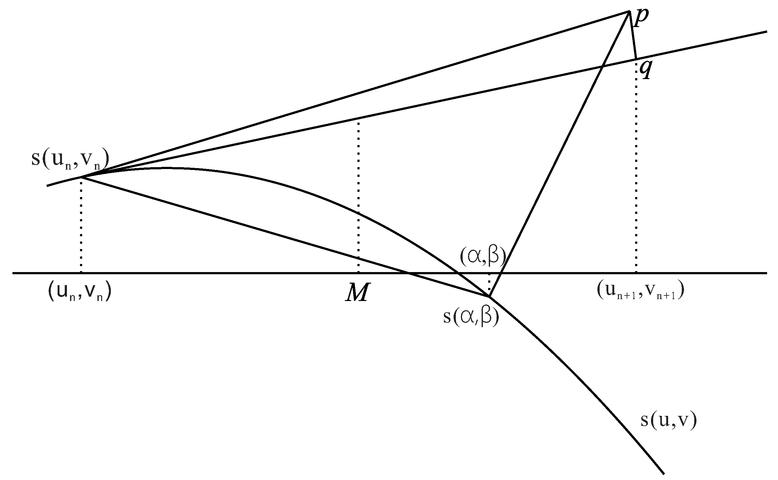
Figure 3.
Illustration of Example 1.

Figure 4.
Illustration of Example 2.

Figure 5.
Graphic demonstration for the hybrid second-order algorithm.


Table 1.
Running time (in nanoseconds) for different initial iterative values by the First-Order method.
Table 1.
Running time (in nanoseconds) for different initial iterative values by the First-Order method.
| (1,−2) | (−2,2) | (−2,−2) | (0,0) | (1,1) | (−2,−1) | |
|---|---|---|---|---|---|---|
| 1 | 142,941 | 132,544 | 39,857 | 135,606 | 133,859 | 40,180 |
| 2 | 132,044 | 155,592 | 38,792 | 133,112 | 160,154 | 45,392 |
| 3 | 133,380 | 132,947 | 38,952 | 181,563 | 132,472 | 46,018 |
| 4 | 132,869 | 140,089 | 43,009 | 132,702 | 133,377 | 40,517 |
| 5 | 134,137 | 134,045 | 40,559 | 134,416 | 125,638 | 39,725 |
| 6 | 136,875 | 140,145 | 43,830 | 146,907 | 132,289 | 41,029 |
| 7 | 133,808 | 133,415 | 39,890 | 132,827 | 133,388 | 40,389 |
| 8 | 132,753 | 148,692 | 41,072 | 133,869 | 135,500 | 44,930 |
| 9 | 132,332 | 153,146 | 38,907 | 1373,30 | 141,663 | 41,428 |
| 10 | 136,460 | 147,361 | 45,462 | 132,184 | 142,250 | 44,384 |
| Average time | 134,760 | 141,798 | 41,033 | 140,051 | 137,059 | 42,399 |
Table 2.
Running time for (in nanoseconds) for different initial iterative values by the First-Order method.
Table 2.
Running time for (in nanoseconds) for different initial iterative values by the First-Order method.
| (1,1) | (2,2) | (2,0) | (1,2) | (2,1) | (0,2) | |
|---|---|---|---|---|---|---|
| 1 | 567,161 | 492,909 | 550,174 | 349,185 | 384,516 | 4,920,804 |
| 2 | 575,759 | 521,233 | 492,835 | 385,293 | 390,527 | 523,743 |
| 3 | 484,250 | 381,832 | 487,414 | 389,792 | 502,568 | 498,248 |
| 4 | 499,588 | 346,864 | 434,103 | 494,559 | 436,330 | 536,043 |
| 5 | 456,397 | 433,893 | 463,222 | 501,650 | 493,197 | 434,355 |
| 6 | 517,495 | 433,521 | 440,372 | 435,692 | 399,478 | 362,600 |
| 7 | 488,340 | 452,431 | 489,985 | 439,752 | 471,909 | 524,395 |
| 8 | 499,700 | 475,481 | 481,180 | 433,924 | 473,261 | 522,088 |
| 9 | 438,441 | 386,592 | 438,255 | 503,681 | 366,078 | 469,647 |
| 10 | 481,179 | 483,391 | 532,150 | 524,016 | 349,502 | 517,721 |
| Average time | 500,831 | 440,815 | 480,969 | 445,755 | 426,737 | 488,092 |
Table 3.
Running time (in nanoseconds) for different initial iterative values by the hybrid second-order algorithm.
Table 3.
Running time (in nanoseconds) for different initial iterative values by the hybrid second-order algorithm.
| (1,−2) | (−2,2) | (−2,−2) | (0,0) | (1,1) | (−2,−1) | |
|---|---|---|---|---|---|---|
| 1 | 321,617 | 298,224 | 89,679 | 305,115 | 301,183 | 90,406 |
| 2 | 297,101 | 350,084 | 87,282 | 299,503 | 360,347 | 102,133 |
| 3 | 300,105 | 299,131 | 87,643 | 408,517 | 298,064 | 103,542 |
| 4 | 298,957 | 315,201 | 96,771 | 298,580 | 300,100 | 91,164 |
| 5 | 301,810 | 301,603 | 91,259 | 302,437 | 282,687 | 89,383 |
| 6 | 307,970 | 315,327 | 98,618 | 330,541 | 297,651 | 92,317 |
| 7 | 301,068 | 300,185 | 89,754 | 298,861 | 300,125 | 90,876 |
| 8 | 298,695 | 334,557 | 92,413 | 301,206 | 304,875 | 101,094 |
| 9 | 297,748 | 344,580 | 87,542 | 308,994 | 318,743 | 93,215 |
| 10 | 307,036 | 331,563 | 102,291 | 297,415 | 320,064 | 99,865 |
| Average time | 303,210.7 | 319,045.5 | 92,325.2 | 315,116.9 | 308,383.9 | 95,399.5 |
Table 4.
Running time (in nanoseconds) for different initial iterative values using the hybrid second-order algorithm.
Table 4.
Running time (in nanoseconds) for different initial iterative values using the hybrid second-order algorithm.
| (1,1) | (2,2) | (2,0) | (1,2) | (2,1) | (0,2) | |
|---|---|---|---|---|---|---|
| 1 | 1,276,113 | 1,109,047 | 1,237,892 | 785,668 | 865,161 | 1,107,181 |
| 2 | 1,295,460 | 1,172,776 | 1,108,880 | 866,911 | 878,687 | 1,178,422 |
| 3 | 1,089,563 | 859,122 | 1,096,683 | 877,034 | 1,130,779 | 1,121,060 |
| 4 | 1,124,075 | 780,446 | 976,732 | 1,112,759 | 981,744 | 1,206,097 |
| 5 | 1,026,895 | 976,261 | 1,042,251 | 1,128,713 | 1,109,694 | 977,300 |
| 6 | 1,164,364 | 975,423 | 990,837 | 980,309 | 898,827 | 815,852 |
| 7 | 1,098,765 | 1,017,971 | 1,102,468 | 989,442 | 1,061,796 | 1,179,891 |
| 8 | 1,124,327 | 1,069,834 | 1,082,657 | 976,331 | 1,064,839 | 1,174,699 |
| 9 | 986,493 | 869,833 | 986,075 | 1,133,284 | 823,676 | 1,056,707 |
| 10 | 1,082,654 | 1,087,631 | 1,197,338 | 1,179,038 | 786,381 | 1,164,873 |
| Average time | 1,126,871 | 991,834.4 | 1,082,181 | 1,002,949 | 960,158.4 | 1,098,208 |
© 2017 by the authors. Licensee MDPI, Basel, Switzerland. This article is an open access article distributed under the terms and conditions of the Creative Commons Attribution (CC BY) license (http://creativecommons.org/licenses/by/4.0/).
Share and Cite
MDPI and ACS Style
Li, X.; Wang, L.; Wu, Z.; Hou, L.; Liang, J.; Li, Q. Hybrid Second-Order Iterative Algorithm for Orthogonal Projection onto a Parametric Surface. Symmetry 2017, 9, 146. https://doi.org/10.3390/sym9080146
AMA Style
Li X, Wang L, Wu Z, Hou L, Liang J, Li Q. Hybrid Second-Order Iterative Algorithm for Orthogonal Projection onto a Parametric Surface. Symmetry. 2017; 9(8):146. https://doi.org/10.3390/sym9080146
Chicago/Turabian StyleLi, Xiaowu, Lin Wang, Zhinan Wu, Linke Hou, Juan Liang, and Qiaoyang Li. 2017. "Hybrid Second-Order Iterative Algorithm for Orthogonal Projection onto a Parametric Surface" Symmetry 9, no. 8: 146. https://doi.org/10.3390/sym9080146
Note that from the first issue of 2016, this journal uses article numbers instead of page numbers. See further details here.