Article

Fractionation Trends and Variability of Rare Earth Elements and Selected Critical Metals in Pelagic Sediment from Abyssal Basin of NE Pacific (Clarion-Clipperton Fracture Zone)

1
Institute of Marine and Environmental Sciences, University of Szczecin, Mickiewicza 16, 70-383 Szczecin, Poland
2
Faculty of Navigation, Maritime University of Szczecin, Wały Chrobrego 1-2, 70-500 Szczecin, Poland
3
Interoceanmetal Joint Organization, Cyryla i Metodego 9, 71-541 Szczecin, Poland
4
Department of Environmental Science and Sustainability, University of Maine at Presque Isle, Presque Isle, ME 04769, USA
*
Author to whom correspondence should be addressed.
Minerals 2020, 10(4), 320; https://doi.org/10.3390/min10040320
Submission received: 12 February 2020 / Revised: 31 March 2020 / Accepted: 31 March 2020 / Published: 2 April 2020
(This article belongs to the Special Issue Marine Geology and Minerals)

Abstract

:
The geochemical and mineralogical characteristics of pelagic sediments collected from the Interoceanmetal Joint Organization (IOM) claim area, located in the eastern part of the Clarion-Clipperton Fracture Zone (CCFZ; eastern tropical Pacific), are described in this paper. The concentrations of rare earth elements (REE), as well as other selected critical elements contained in 135 sediment samples of siliceous clayey silts, are presented. The vertical and spatial variabilities of elements, with particular emphasis on REE as well as metals of the highest economic interest such as Cu, Ni, and Co, are detailed. The applied methods include grain size analysis by laser diffraction, geochemistry examination using ICP-MS, XRF, AAS, and CNS spectrometry, and XRD analysis of mineral composition (Rietveld method). Additionally, statistical methods such as factor analysis (FA) and principal components analysis (PCA) were applied to the results. Finally, a series of maps was prepared by geostatistical methods (universal kriging). Grain size analysis showed poor sorting of the examined fine-grained silts. ICP-MS indicated that total REE contents varied from 200 to 577 ppm, with a mean of 285 ppm, which is generally low. The contents of critical metals such as Cu, Ni, and Co were also low to moderate, apart from some individual sampling stations where total contents were 0.15% or more. Metal composition in sediments was dominated by Cu, Ni, and Zn. A mineral composition analysis revealed the dominance of amorphous biogenic opaline silica (27–58%), which were mostly remnants of diatoms, radiolarians, and sponges associated with clay minerals (23% to 48%), mostly Fe-smectite and illite, with mixed-layered illite/smectite. The high abundance of diagenetic barite crystals found in SEM−EDX observations explains the high content of Ba (up to 2.4%). The sediments showed complex lateral and horizontal fractionation trends for REE and critical metals, caused mostly by clay components, early diagenetic processes, admixtures of allogenic detrital minerals, or scavenging by micronodules.

Graphical Abstract

1. Introduction

1.1. General Physical and Chemical Behavior of Rare Earth Elements

Rare earth elements (REE), also called rare earth metals, comprise the 15 lanthanides with atomic numbers from 57 to 71, i.e., lanthanum, cerium, praseodymium, neodymium, promethium, samarium, europium, gadolinium, terbium, dysprosium, holmium, erbium, thulium, ytterbium, lutetium, as well as two nonlanthanide elements that have properties that are similar enough to allow them to be included in this set, i.e., scandium and yttrium. Promethium, which may be formed in nuclear reactions, does not naturally occur on Earth in significant quantities [1]. REEs have unique chemical similarities, being usually divided into light (LREE = Light Rare Earth Elements; La to Gd) and heavy (HREE; from Tb to Lu and Y). Sometimes added is a “medium” (MREE; Eu to Er) division [2].
REEs are considered hydrolysates, since ions are easily hydrolyzed in aqueous solutions. In lanthanides, the pH of hydrolysis ranges from 8 for La to 6.2 for Lu. Therefore, REEs can be fractionated by hydrolysis in natural solutions over a large pH range. Due to small REE amounts in rocks and waters, lanthanide mobility in natural processes is more often controlled by the ability to form compounds from organic and inorganic ligands than by dissolving components. This capacity increases with the reduction of ion beams from HREE to LREE, which results in increased HREE content in standard charts, including sea water. However, average concentrations in porewater do not show this trend [3]. Limited REE mobility is associated with adsorption tendency on solid particles, mostly due to ion pair formation on the surface of particles, or simultaneous precipitation during the formation of solid phases, mainly due to subsequent isomorphic exchange and the adsorption on newly formed solid phases [4].
In sediments, sedimentary rocks, and sea water, most lanthanides indicate +3 oxidation state, with exceptions being Ce and Eu. Under aerobic conditions, trivalent cerium can be oxidized to Ce4+, and form compounds that are sparingly soluble (mainly CeO2). Therefore, oxygenated water is depleted of complexion, that is enriched in oxygenated sediments. Similarly, in hypoxic water (under suboxic conditions), suspended Ce is mobilized and thus released, while in anaerobic sediments, Ce deficiency usually occurs [5]. This phenomenon of the enrichment or depletion of Ce in relation to neighboring REE is called a positive or negative Ce anomaly (Cean). The value of Cean = 1 means that Ce is not different from the mean concentration in standard samples. Cean < 1 is a negative Cean, while Cean > 1 indicates enriched Ce [6]. The highest Cean is characteristic for hydrogenetic cobalt-rich crusts, phosphatized crusts, as well as hydrogenetic polymetallic nodules and micronodules. Diagenetic nodules exhibit a small positive or even negative Cean, while fast growth rate crusts located in the immediate vicinity of hydrothermal sources, as well as carbonate sediments and seawater, are usually characterized by a negative Cean [7,8]. Pelagic clays are mostly characterized by a positive Cean and elevated MREE level, mainly due to the extraction of lanthanides from seawater by hydrogenic iron oxyhydroxides, and in case of Ce, also by manganese oxyhydroxides. In the sea water column, an increase of dissolved REE at below surface-depth due to the desorption of suspended REEs is noted, and the lowest value of a negative Cean usually occurs at ~200–300 m, which is directly associated with the upper oxygen minimum zone (OMZ). Therefore, the Cean reflects the redox reactions in both water and sediments [6].
Eu also occurs at two oxidation levels (+2 and +3), and enrichment or deficiency also leads to the formation of a positive or negative Euan, which can be an indicator of the inflow to sedimentation zones of abyssal material usually derived from hydrothermal solutions, fluids, volcanic rocks, and fragments of alkaline rocks [9]. A positive Euan is an indicator of high-temperature hydrothermal solutions (as a result of water-basalt reaction), and may be associated with hydrothermal transformations of sedimentary rocks. A low positive Euan is characterized by diagenetic nodules [8]. The supply of suspended and dissolved material in rivers, which is subordinately supplemented by aeolian material, the halmyrolysis of igneous rocks, or hydrothermal processes, is considered to be the main REE source in sea water. Evidence exists of the hydrothermal origin of REE-enriched sediment in LREE, especially Eu, which occurs at the +2 degree of oxidation in hydrothermal solutions (T = 300 °C to 400 °C and pH ~3). At the same time, the REE content increases as the fluid temperature increases, while pH decreases [4].

1.2. REE in Deep-Sea Sediments

Since the widely cited work of [10], deep-sea sediments have been the subject of numerous studies focused on REE content and resource potential [11,12,13,14,15,16,17,18,19,20]. According to [10], who analyzed 2000 seafloor sediment samples at 78 Pacific sites, deep-sea muds show high concentrations of ∑REE (2230 ppm maximum), and could constitute a potential source of these elements in the future. Such high REE concentrations in sediments were not confirmed either by the studies of [21], who studied samples from the central North Pacific, or [16], who examined material collected from the southern part of the Korean claim area (KORDI) of the Clarion–Clipperton Fracture Zone (CCFZ). The former research has shown that total REE contents vary from 418 ppm to 810 ppm, with an average of 532 ppm, while the latter recorded a range from 115 ppm to 1115 ppm, with an even lower average of 490 ppm. Higher REE concentrations occur at other central North Pacific locations, ranging from 439 to 1654, and with a mean of 790 ppm [22,23], and demonstrate that REE concentrations and fractioning are determined by geodynamics and hydrological processes. These include mostly sediment depth and distance from hydrothermally active areas, depositional regime parameters (sedimentation rate, admixtures of biogenic material), or the intensity and distributional patterns of seafloor currents. Effects on the sedimentary environment are manifested here by positive correlations between LREE/HREE and grain size composition, Rb/Sr and Nb/Y values, and negative correlations with Zr/Rb values. Elevated contents of HREE rarely occur in deep-sea basins, where mostly biogenic and organic silts are accumulated. The HREE depletion is related to a lower amount of terrigenous components such as zircon, and other detrital or mantle sourced minerals [24]. A different noneconomic application was proposed for REE by [25], who described foraminiferal REE signatures (especially HREE/LREE, MREE/MREE*) as indicators of large-scale changes in ocean circulation (water mass provenance and mixing) in the past.
Several authors have attempted to determine the main carrier of REE in deep-sea sediments. Due to the mineralogical composition of pelagic sediments, major components are classified as biogenic, lithogenic (detrital or allogenic), and hydrogenic (forming in situ, absorptive or authigenic). Several of these possess individual geochemical signatures related to formation conditions [26]. REE distribution in polygenetic pelagic sediments results from terrigenous, biogenic, hydrogenic, volcanogenic, and hydrothermal components that influence specific REE compositions. Moreover, diagenetic processes produce new mineral phases, such as barite, zeolites, ferromanganese micronodules, and apatite, which host remobilized REE [4].
Most researchers claim that hydrothermal Fe–Mn oxyhydroxides, as well as zeolites (mostly phillipsite), are the main host phases for REE [10], however, zeolites can also form as a diagenetic product, being considered rather as an indicator of burial diagenesis (similarly to barite) than the major host of REE [4]. Additional recent studies provide new evidence for relatively high REE concentrations in bioapatite (fish debris, mostly teeth and bones) [21,27,28]. These observations support conclusions that during oxic diagenesis, REE which initially had adsorbed into Fe–Mn minerals (mostly vernadite, birnessite and todorokite) were later released into pore waters, and resorbed by apatite [22,29]. Additionally, REE sources may be related to Fe-rich authigenic (diagenetic) clay minerals and admixtures of allogenic components from continental areas [14,19,30]. The REE accumulation in pelagic sediments may also be related to external influx of Fe/Mn-microparticles [31]. The REE composition and distributional patterns may be also related to high temperature hydrothermal iron oxides and aluminosilicates, products of bedrock disintegration, or endogenous (volcanoes) and exogenous (desert dust) components [32].

1.3. REE in CCFZ

According to factor analyses of chemical sediment components from the northern CCFZ, REE are positively correlated with Fe and Co, which suggests formation to be strongly influenced by hydrogenic processes (slow precipitation of metals from/under influence of seawater), and Ca-phosphate sources. The positive iron and cobalt relation may be the result of Co accommodation in the structure of amorphous Fe-rich gels, with different behavior under redox conditions. The nickel behavior is related to worse oxidation potential, compared to Co, which suggests accumulation within Mn-rich oxyhydroxide structures [33]. At the same time, REE show positive correlations with Al, K, and Ti, and negative correlations with Cu and Ni, which may suggest the influence of detrital material. Positive relations between Mn, Ba, Sr, Ni, and Cu are considered to be a diagenetic process effect [34]. Ni and Cu are related mostly to slow hydrogenic Mn-oxyhydroxide growth. Ba is usually included in diagenetic barite. Sr may be related to vacancy places in barite, or as small impurities in clay minerals or zeolites. The enrichment mechanism of REE in pelagic siliceous clayey silts from the western CCFZ is characterized by REE contents between 400 and 1000 ppm and significant negative Cean [35].
REE and metal contents are usually related to Fe variations in interstitial water, which are strong reducing agents. The development of reducing conditions in sediment leads to an increase in Ce and LREE. The change from reducing oxidizing conditions promotes a more prominent decrease in Ce and LREE relative to HREE. A sharp rise of Ce content is related to reduction and transfer from solid sediment phases into interstitial water. LREE displays the lowest mobility during diagenesis. The accumulation of phosphates from interstitial water on diagenetic iron oxyhydroxide leads to additional extraction of HREE [4,36]. The development of reducing conditions in sediments is related to the oxidation of organic matter with oxidants including dissolved oxygen, nitrates, Mn+4 oxyhydroxides, Fe+3 oxyhydroxides, or sulfates [37].
The relationship between sedimentation rate, local hydrodynamics and pore-water geochemistry, with respect to the nodule coverage in CCFZ, has been studied by numerous authors [38,39]. The results indicate that sites entirely without nodules, or with only small ones, are characterized by higher sedimentation rates, lower contents of leachable manganese, and higher rates of nitrate and manganese oxide reduction below the oxygen penetration depth. These sites are also characterized by increased proportions of fine-grained sediment at the surface, a lower content of mobilizable authigenic manganese, and higher amounts of refractory manganese. Different coarse-grained particles, with higher amounts of leachable manganese and lower amounts of refractory manganese, occur in regions with large and medium-sized nodules [39]. Manganese mobilization in CCFZ sediment was and is strongly affected by shifts of oxic–suboxic redox boundary and bioturbation intensity [40], especially during Late Pleistocene-Holocene [41].
The main aim of this paper is to present a geochemical and mineralogical description of 135 sediment samples of siliceous clayey silts collected from the abyssal basin of NE Pacific (Clarion–Clipperton Fracture Zone). This study presents the vertical and spatial variability of selected metal contents, with the main emphasis placed on REE, Cu, and Ni, as well as Co and other metals. The relations between grain size, depth in the sediment column, and mineral and chemical compositions are also discussed, with special emphasis on neighboring polymetallic nodules polygons and the metal-rich sediments of the central Pacific.

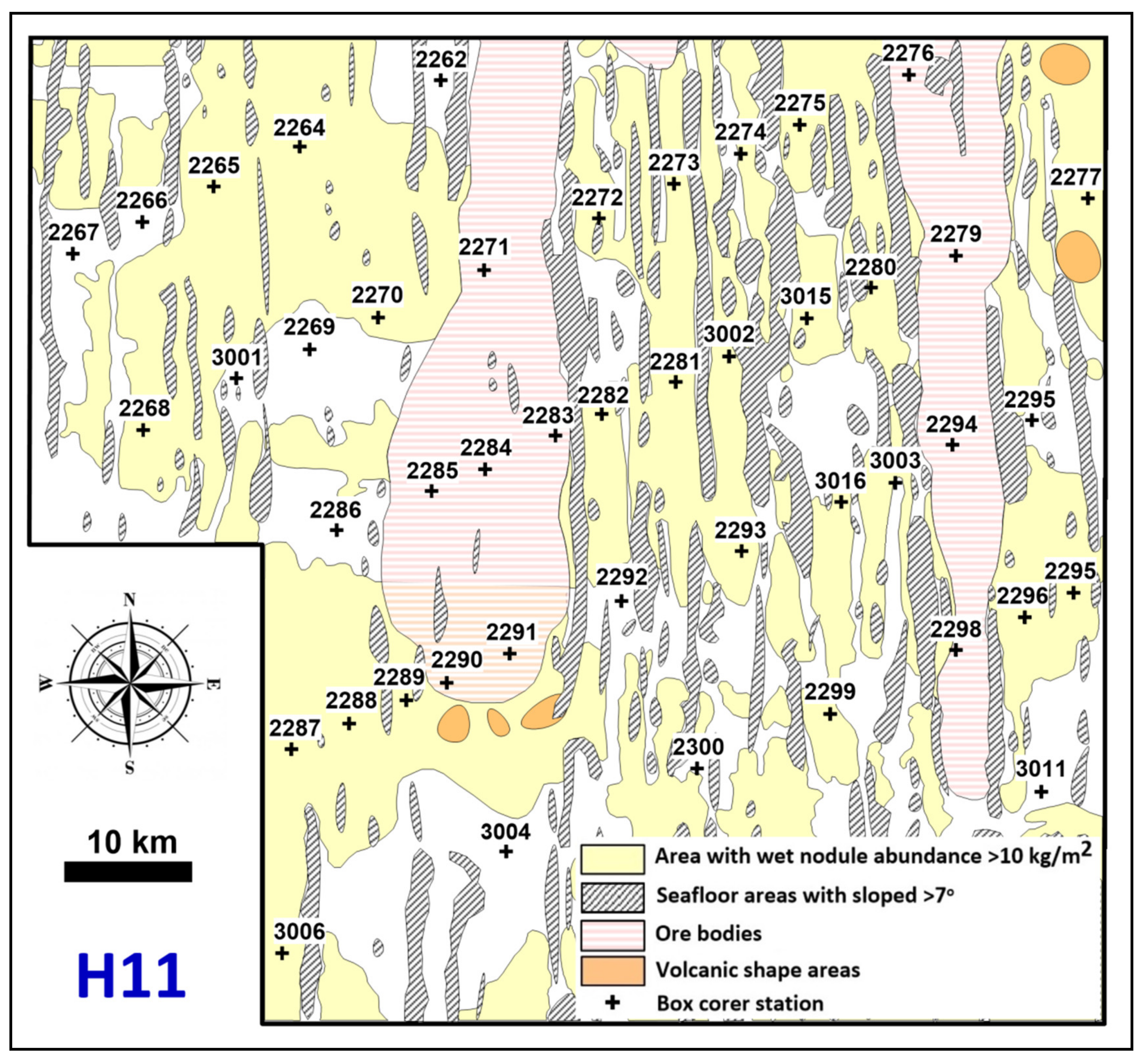
2. Geological Setting

CCFZ is located in the northeast equatorial Pacific abyssal basin, between two fractures: (i) Clarion to the north, and (ii) Clipperton to the south (Figure 1). The CCFZ area is approximately 5.5 million km2, extending 5200 km between 116° W and 155° W, and 1000 km between 5° N and 15° N. To the east, the zone bounds the Mathematicians Ridge (MR), which is believed to be the Paleo-East Pacific Rise (PEPR) western slope, west of the Line volcanic island arc [42,43].
Since the greatest concentrations of polymetallic nodules (PM) have been discovered in the CCFZ, this region has the best prospects for future deep-sea mining [46,47]. The PM are formed there mostly by hydrogenetic accretion and oxic-suboxic diagenesis [48]. Due to the great interest in PM, CCFZ is one of the better-known areas of ocean floor. Cartographic, bathymetric, seismic, sedimentological, economic, and environmental research have been conducted in this area since the mid-1960s [38,49,50]. This region is under the jurisdiction of the International Seabed Authority (ISA), Kingston, Jamaica, which has entered into 15-year contracts for exploration for polymetallic nodules with sixteen contractors [51].
The CCFZ geomorphological structure conforms to the pattern of a typical seabed structure for mid-ocean ridges and adjacent basins. A gradual increase of average depth from 3800–4200 m at 115° W to 5400–5600 m is observed to the West. The average slope varies from 0.57° in the east, to less than half a degree in the western part. Several volcano-tectonic units have been identified, such as the Cooper Rise, Central Rise, East Rise, and Shimada Seamount. In addition to these features, the seafloor is characterized by a regular bathymetric pattern that consists of a system of adjacent linear groups of ridges and valleys, aligned approximately perpendicular to the boundary between the Clarion and Clipperton Fracture Zones. Distances between neighboring crests vary from 1 to 10 km, with elevations above surrounding terrain up to hundreds of meters [31]. The CCFZ ocean crust is 10.6–10.8 km thick, and is composed of two complexes: (i) tholeiitic basalts, and (ii) overlying sediment cover, with a thickness of 100 to 300 m, and age range from Late Cretaceous to Quaternary [43,52].
The surface sediments within CCFZ are characterized by zonal distribution, and are represented by two classes with a few subclasses of biogenic sediments: (i) carbonate sediments, within which carbonate silts and clays, as well as carbonate oozes can be distinguished, and (ii) siliceous sediments (mostly red clays, diatom-radiolarian silts and oozes). Mixtures of these two end-members are predominant across the vast majority of the CCFZ seabed. Additionally, some minor sediment types are recognized, such as zeolitic clays or sediments heavily enriched with volcanic and hydrothermal components [52]. The carbonate compensation depth (CCD) ranges from 4000 to 4500 m, and is deepest in the westernmost CCFZ, shallowing towards the western Central America coast [42,53].
The surface sediments were classified using the Clarion lithostratigraphic groups, with three formations distinguished: (i) Line (FL), (ii) Marquise (FM), and (iii) Clipperton (FCl). FL is mostly represented by zeolitic clays, diatom-radiolarian silts, and siliceous silty clays, which are of the late Eocene and Oligocene ages. Based on the lithological composition of sediments and genesis within the formation, four lithostratigraphic units were distinguished: (i,ii) Marquise: FM I and FM II, (iii) Clipperton FCl III, and (iv) FCl IV [42,54].
The sediments studied in this paper belong to the FCl IV unit, characterized by considerable lithological variability, the largest thickness of all units, as well as a macroscopically visible zonation. This unit is mostly represented by calcareous silty clays (up to 47% of CaCO3), and Ethmodiscus silty clays (up to 32% of SiO2am). The uppermost horizon, the so-called semiliquid geochemically active sediment layer, is composed of two types of sediments: (i) siliceous silty clays (up to 30% SiO2am), and (ii) slightly siliceous clayey silts (less than 10% SiO2am). Sedimentation of this unit began during Pliocene and continues to this day [42]. Biological productivity and organism activity in CCFZ sediment is high in comparison with other oceanic basins [55]. Due to the higher biologically related uptake of nutrients, such as C, N, P, Si, and Ca in surface water, and the further remineralization in deepwater, the REE and metals accumulated more extensively in deeper Pacific basins compared to those in the Atlantic Ocean [56].
Sixteen contractors signed 15-year contracts for exploration for polymetallic nodules in the CCFZ. One of the first was the Interoceanmetal Joint Organization (IOM), a consortium of six states: Bulgaria, Cuba, Czech Republic, Poland, Russia, and Slovakia. The IOM exploration area is located in the eastern CCFZ and is composed of two separate blocks, B1 and B2, with a total area of 75,000 km2. Samples studied in this paper come from the IOM H11 exploratory area (located in B2; Figure 1) which constitutes a polygon that covers 5380 km2, and is rich in PM. The seafloor topography is dominated by elongated, streaked, and rounded patchy-like zones, showing high nodule coverage (>13 kg/m2). Nodule-free sites are usually covered by soft siliceous-clayey sediments, often associated with high biogenic productivity or erosional near-bottom currents [46,57].

3. Materials and Methods

3.1. Sample Collection and Processing

A total of 135 samples from 45 sampling sites were collected in 2009 using a Reineck box corer (Ocean Instruments, Fall City, WA, USA), during the IOM research R/V “Yuzhmorgeologiya”, in the IOM H11 polygon (Figure 2). The surface area of the box corer is 0.25 m2 and the maximum penetration depth 0.5 m, from where nondisturbed soft sediments were taken for analysis. Samples were recovered at a depth range from 4313 to 4529 m. The investigated sediments are mostly siliceous-clayey silts.
Based on macroscopic description, the samples were divided onboard into four horizons (called here also layers or sections). The main criteria were: (i) the sediment color, (ii) water content, and (iii) sediment consistency (Figure 3):
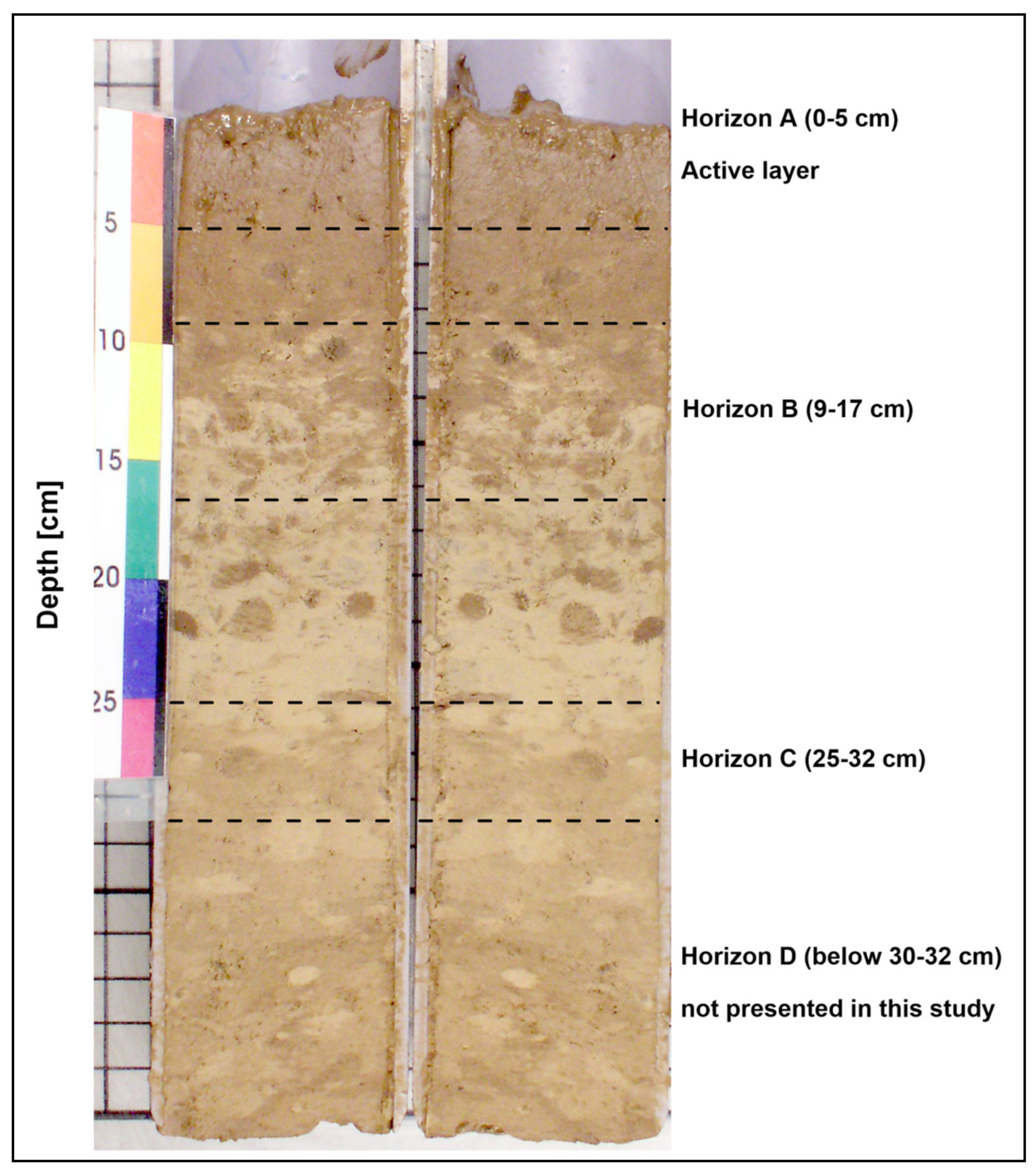
  • horizon A—semiliquid geochemically active surface layer (0−5 cm; number of samples: 45), subsequently called “active layer” [43]. This horizon contains the highest amount of nonburied polymetallic nodules, which were removed from the samples before analysis. The horizon is characterized by a dark brown to brown color, the highest water content, and friable consistency.
  • horizon B—the upper part of the middle section (9−17 cm; n = 45). This layer is transitional between the uppermost semiliquid horizon A and the denser horizon C below. This sediment is beige with brownish bioturbation traces, lower water content than the uppermost layer, and is also more firm.
  • horizon C—the intermediate part of the middle section, (25−32 cm; n = 45). Sediment is dark beige with some brownish bioturbation traces, moderate water content, and greater firmness compared to horizons A and B.
  • horizon D—the lower part of the middle section (below 30–32 cm; up to 42 cm, n = 2). The horizon with the lowest water content and greatest firmness.
Since the number of horizon D samples is too few for separate statistical analyses, this interval is omitted in the present study.
The data analysis included sedimentological (laser grain size analysis), mineralogical (powder X-ray diffraction—XRD), and geochemical (Energy Dispersive X-ray Fluorescence—EDXRF) laboratory methods, as well as Atomic Adsorption Spectrometry (AAS), Carbon-Nitrogen-Sulphur spectrometry (CNS), flow-injection phosphorus photometry (FIA), and Inductively Coupled Plasma Mass Spectrometry (ICP-MS).

3.2. Grain Size Distribution Analysis

The sediment grain size distribution was analyzed by laser-aided measurements using a Malvern Micro Analyzer 300 at the Institute of Marine and Environmental Sciences, University of Szczecin (IMES-USz, Szczecin, Poland). The lyophilized sediment samples were placed in 500 mL glass beakers filled with distilled water.
For better fractionation of sediments, samples were subjected to a 4-min water-based ultrasonic disintegration treatment, at a sound frequency of 20 kHz and water pump speed of 2000 rpm [59]. Each sample was treated with a 7 mL 1.6% sodium pyrophosphate dispersant solution. Analytical data were processed by the Malvern software (Malvern Panalytical Ltd., Malvern, UK) with conversion of values (for best optical laser coefficient) to the polydispersed illite + sodium pyrophosphate dispersion model [60]. The grain size analysis was recalculated using the Gradistat software (version 8, Kenneth Pye Associates Ltd., Shinfield, UK) in order to obtain the basic statistical grain size parameters. Grain size results use the φ unit according to formula (1) [61,62]:
ϕ = −log2D (mm),
where D is mean grain size (mm).

3.3. Mineralogy

The bulk of the mineralogical XRD analysis was done on 41 selected samples, using a PANalytical Empyrean diffractometer (Malvern Panalytical Ltd., Malvern, UK). The analytical settings were as follows: monochromatic CuK-α radiation at 35 kV and 30 mA, scans from 5–70° (2θ), step size 0.024 (2θ), using a wide angle detector (PIXcel 3D), conducted at the Faculty of Chemical Technology and Engineering, West Pomeranian University of Technology, Szczecin, Poland (WPUT). The X-ray diffraction results were recalculated using the Rietveld method and the RockJock software (version 11) [63]. The amorphous silica content was estimated as a background increase observed in X-ray diffractograms [64]. Due to the high resolution of obtained bulk diffractograms, clay minerals separation for further analyses was omitted. Also, no chemical treatment was applied to the clays. The matching of clay polytypes was done based on earlier experiments by Maciąg et al. [65], where separated clay subfraction <0.004 mm was heated, oriented, and glycolyzed. A quantitative analysis was performed based on the repetitive calculation of patterns (around 7 to 9 iterations), and finally, by comparison with experimental patterns, according to highest fit quality, expressed by the lowest residuals and highest goodness of fit. Kaolinite and chlorite were identified by the presence or absence, and the position, of the first low angle diffraction peak (~10Å for kaolinite, 14–14.2Å for chlorites).

3.4. Geochemistry

The contents of major elements (Fe, Mn, Si, Al, Na, Mg, Ca, K, Ti, Cl, P, and S) in 10 samples were determined by EDXRF analyses of powdered and press-pelleted samples, following [56], and using a PANalytical Epsilon 3 EDXRF spectrometer (Malvern Panalytical, Royston, UK), at WPUT.
Iron and manganese contents were analyzed by the AAS method at IMES-USz. The 30 sediment samples (each 0.6 g) were digested using a microwave oven with a mixture of three acids: 8 mL HNO3 65%, 2 mL HCl 10%, and 2 mL H2O2 30% [60]. The analysis was performed with a Unicam Solaar 969 flame atomization spectrometer. Biogenic element concentrations (TC, TN, TS) were analyzed at the same institute, using the same number of samples, by CNS spectrometry on a Vario MAX CNS Element Analyzer [66]. The total phosphorus content was estimated for 30 samples with the flow-injection absorbance photometric method (FIA), using an MLE photometer (Germany) [67]. Before measurement, samples were mineralized as AAS, with analyses also being conducted at IMES-USz.
A minor and trace elements analysis, including REE, was done on 135 samples. The elements were determined following [68] and after full acid digestion (HNO3, HF, HClO4 and Aqua Regia), by ICP-MS (ELAN DRC II, Perkin Elmer, Waltham, MA, USA), at the Central Chemical Laboratory, Polish Geological Institute—National Research Institute (PGI-NRI), Warsaw, Poland. The ICP-MS data were normalized to the Post Archean Australian Shale (PAAS) [69]. To show differences in normalization standards, the eight most characteristic samples were normalized to the World Shale Average (WSA) [70], North American Shale Composite (NASC) [71], Upper Continental Crust (UCC) [72], PAAS, and chondrite [73].
To determine the individual sediment component groups and sample imaging, we used a Hitachi SU8020 ultrahigh-resolution field-emission scanning electron microscope (UHR FE–SEM, Hitachi High-Technologies Corporation, Tokyo, Japan). For analysis, material was separated by water flushing of selected samples with a ϕ = 0.063 mm sieve, or by gravitational sedimentary suspension in a glass cylinder filled with distilled water. The Energy-Dispersive X-rays (EDX) spectra were collected and analyzed in the NSS 3.0 software. The data were collected at WPUT.

3.5. Data Processing

Maps, graphs, and lithological profiles were prepared using the Surfer 9, Grapher 10, and Strater 4 software (Golden Software Inc., Golden, CO, USA). The basic statistics for the total population and each sampling level were calculated separately, using Statistica Statsoft 7 (Statsoft, Tulsa, OK, USA). Construction of correlation coefficient matrices used 45 samples within each sampling interval. Valid cases were presented for p = 0.95, and were compared/removed pairwise. Factor analysis (FA) and principal components analysis (PCA) were performed separately for each horizon. The final components were expressed by normalized varimax rotation. A comparison of the same statistical data within all sampling horizons determined the number and types of geological factors and potential influences of each factor on metal scavenging processes.
The generalized maps of mean grain size, total contents of Cu, Ni, and Co, total REE, and amorphous SiO2/clay minerals ratio were made using the geostatistical methods available in Golden Software Surfer 9 software. Because of the observed significant spatial data trend and drift, universal kriging was applied for contouring. The basic trend maps were constructed using simple polynomial 1st (one directional variability), or binominal 2nd degree functions (two-directional variability). Afterwards, omnidirectional variogram models were constructed for each map. We applied the linear trend equation as the drift function [74]. For two maps (total content of metals in horizons B and C), anomalous data points were removed from the data set. For maps of grain size, metals, and ∑REE distribution, the full data set of 45 samples was used. In the case of amorphous SiO2 and clay minerals ratio, maps were produced using data from 13 sample stations.
The use of geostatistical methods is not the main topic of this paper; therefore, similar or more detailed information about spatial modelling in the study area can be found in [75,76,77].
Additionally, normalized REE spider diagrams were oriented towards the maximum trend directions, and color scale was applied for better geographical presentation. This presentation allowed us to orient normalized REE contents with the spatial directions, and show differences in LREE/MREE/HREE fractionation according to the various data trends.
The cerium Equation (2) and europium anomalies Equation (3), Cean and Euan, respectively, and normalized LREE/HREEPAAS ratio Equation (4) were determined using the following equations [7,78]:
Cean = 2 × Ce/CePAAS/(La/LaPAAS + Nd/NdPAAS),
Euan = 2 × Eu/EuPAAS/(Sm/SmPAAS + Gd/GdPAAS),
(LREE/HREE)PAAS = (La/LaPAAS + 2Pr/PrPAAS + Nd/NdPAAS)/(Er/ErPAAS + Tm/TmPAAS + + Yb/YbPAAS + Lu/LuPAAS).

4. Results

4.1. Grain Size Analysis

The grain size analysis indicated that 90% of studied samples were fine silts. The mean grain size varied from 5.86 to 8.08 φ (x = 6.83 φ), while the median ranged from 5.75 to 8.08 φ (x = 6.97 φ). Around 84% of samples showed unimodal particle size distribution, while 16% were characterized by bimodal distribution. Sorting coefficients varied from 1.06 to 1.82 (x = 1.53); however, in 72% of the samples, sorting was in range of 1.4 to 1.7.
According to classification [61], the sediments under study were poorly sorted. Over 80% of the samples showed coarse-skewness, while the rest were nearly symmetrical. Kurtosis ranged from 0.76 to 1.19 (x = 0.96), where 29% of samples were platykurtic, while the remainder were mesokurtic. Grain size fraction variability in the different depth horizons was mostly similar. The silt and clay content slightly increased in horizon C, while the sandy fraction decreased. The sandy subfraction content (>0.063 mm; <4 φ) in all 135 sediment samples ranged from 0.01 to 17.5% (x = 5.73%), while silt (0.004–0.063 mm; 4–8 φ) varied from 78.26% to 96.36% (x = 89.96%), and clay (<0.004; <8 φ) in 86% of samples ranged from 15% to 30%. The complete sedimentological data for individual horizons A, B, and C is presented in Table S1.

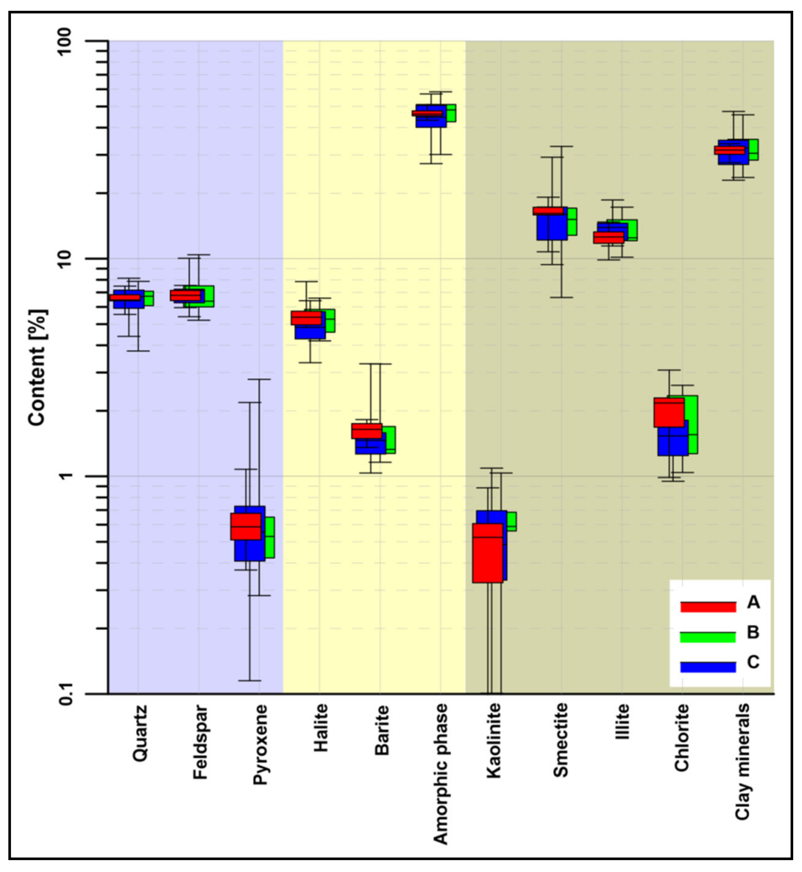
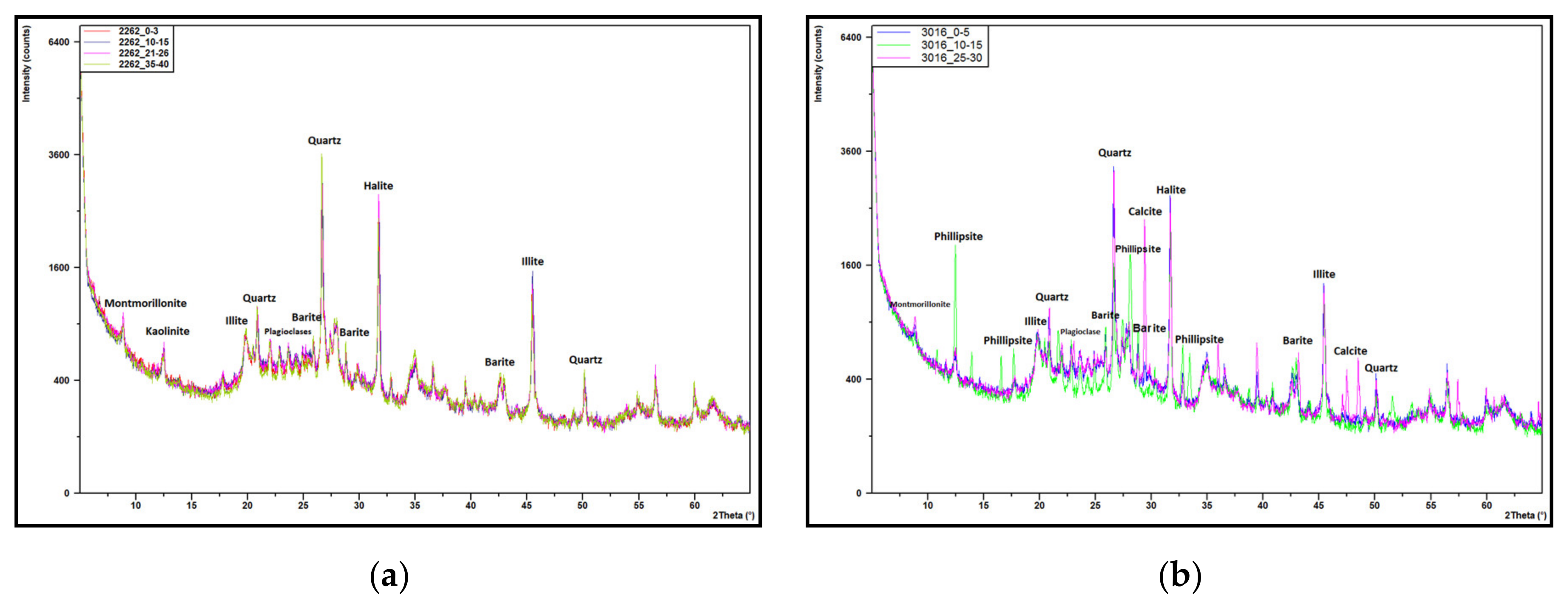
4.2. Bulk XRD Mineralogy

As per the general mineral composition (Figure 4), the analyzed sediments were dominated by amorphous, mostly biogenic opal-A, comprised of radiolarian tests, siliceous sponge spicules, or diatom frustules. Additionally, admixtures of amorphous siliceous volcanic glass with vitreous tephra composition were identified. The amorphous SiO2 content varied from 27% to 58%. The greatest differences in silica content were observed in horizon C, where contents were from 27% to 57%, with a mean of 45%. The horizon B differences were smaller, ranging from 30% to 58%, with a mean of 47%. The differences within the horizon A were small (43–51%), with a mean of 47%. The amorphous silica content decreased slightly in deeper parts of the sediment column.
The clay content varied from 23% to 48%, and showed similar variability to the amorphous silica. Clay showed greatest variability in horizon C, varying from 23% to 48%, with a mean of 32%. The clay minerals content in horizon B was similar, and varied from 24% to 48%, with a mean of 32%. The clay contents within horizon A were less variable (28% to 34%), with a mean of 32%.
The clay minerals were dominated by dioctahedral Fe-smectite (nontronite), illite, and mixed-layered illite-smectite (I-Sm). Smectite generally dominated (6.6% to 32.8%, with a mean of 16.3%); however, increased amounts of smectite and illite were observed in the B and C horizons. Additionally, traces of trioctahedral hectorite and Ca-montmorillonite occurred [79].
Illite was represented by fine-crystalline illite 1Md and detrital illite 1M1 [80]. The total illite contents varied from 10% to 18.7%, with a mean of 13.2%. The content of illite slightly increased within horizon B and C (usually 2–3% more compared to horizon A), mostly due to the illitization process caused by burial diagenesis. The single-layered illite 1M was less represented (usually <2%). Additionally, randomly ordered mixed-layered illite-smectite occurred, with I/S between 0.5 and 0.7 [81].
Kaolinite was usually 1% or less, and represented by disordered kaolinite D [82]. Chlorite was mostly trioctahedral (Mg)/Fe-chlorite (clinochlore-chamosite), with contents between 1% and 3%, and a mean of ~1.5% [83]. Additionally, there was a small quantity (~1%) of mixed-layered 1:1 I/Ch (compare [60,81]).
The important identified diagenetic mineral was barite, with a mean content of 1.6%, and a minimum and maximum of 1.04% and 3.30%, respectively. The barite content in the sediment column was rather stable, though extreme values occurred in horizons B and C, in some cases exceeding 3%.
The other diagenetic mineral was halite, which formed during the removal of interstitial water from sediments, i.e., during sample drying. Halite contents varied from 3.3% to 7.9%, with a mean of 5.2%, and gradually decreased in horizons B and C, mostly due to lower porosity, compared to horizon A.
The allogenic components were represented by detrital quartz (of mostly aeolian genesis), plagioclase, and dark heavy minerals, such as pyroxenes. The quartz and plagioclase contents were quite similar, and varied from 3.8% to 10%, with means of 6.5% and 7.1%, respectively. The plagioclase was mostly of the andesine type, with less bytownite and oligoclase endmembers. The highest plagioclase content occurred in horizon C. Additionally, there were traces of pyroxenes (<1%) augite and enstatite types.
Loose samples from selected sampling stations show the presence of other minerals (Figure 5a,b). For sample 3016 10-15, diffraction peaks of zeolites (phillipsite-Na) were observed, while sample 3016 25-30 showed traces of calcite. Calcite occurred in twelve samples, with contents of up to 9.2%.

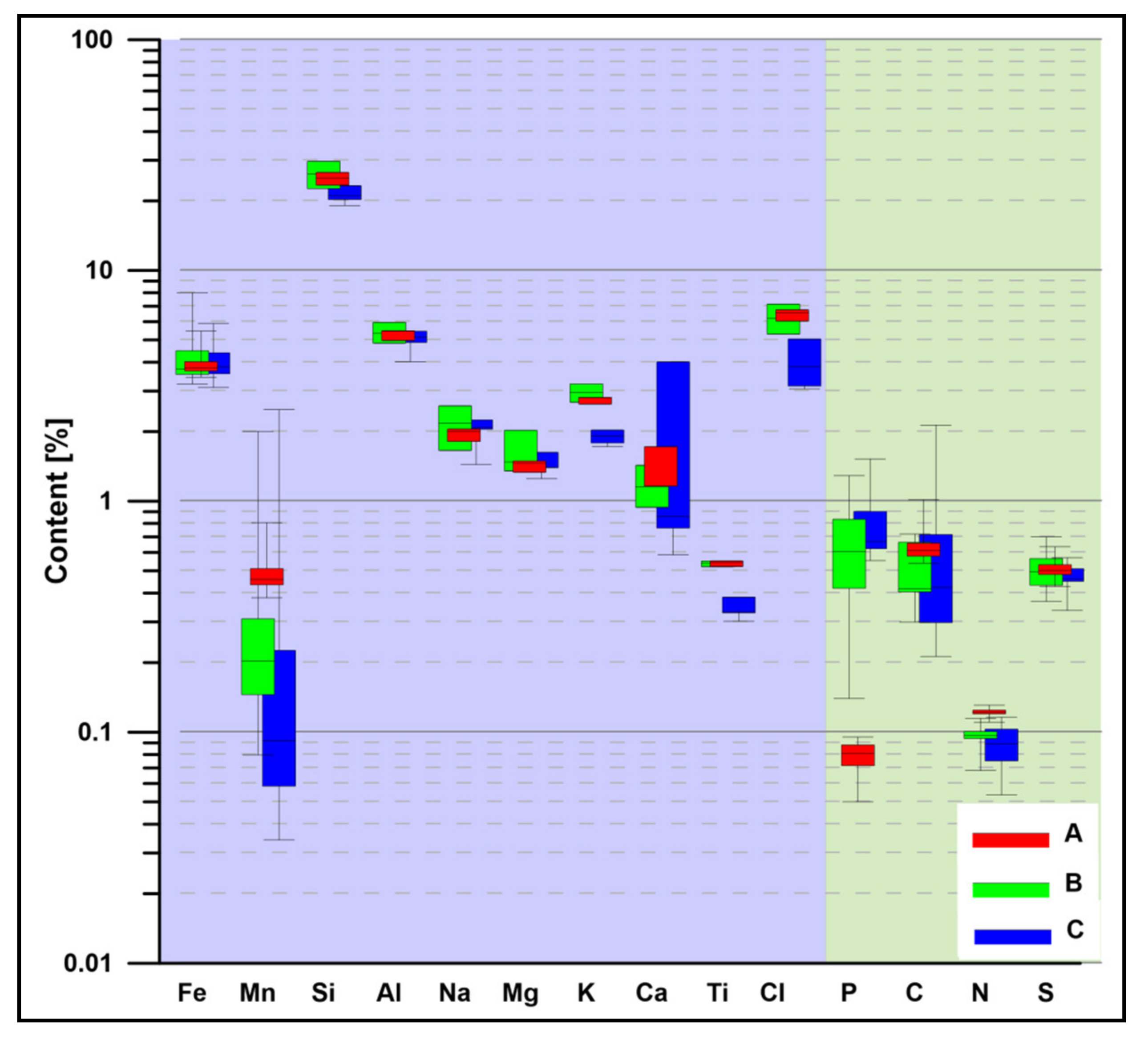
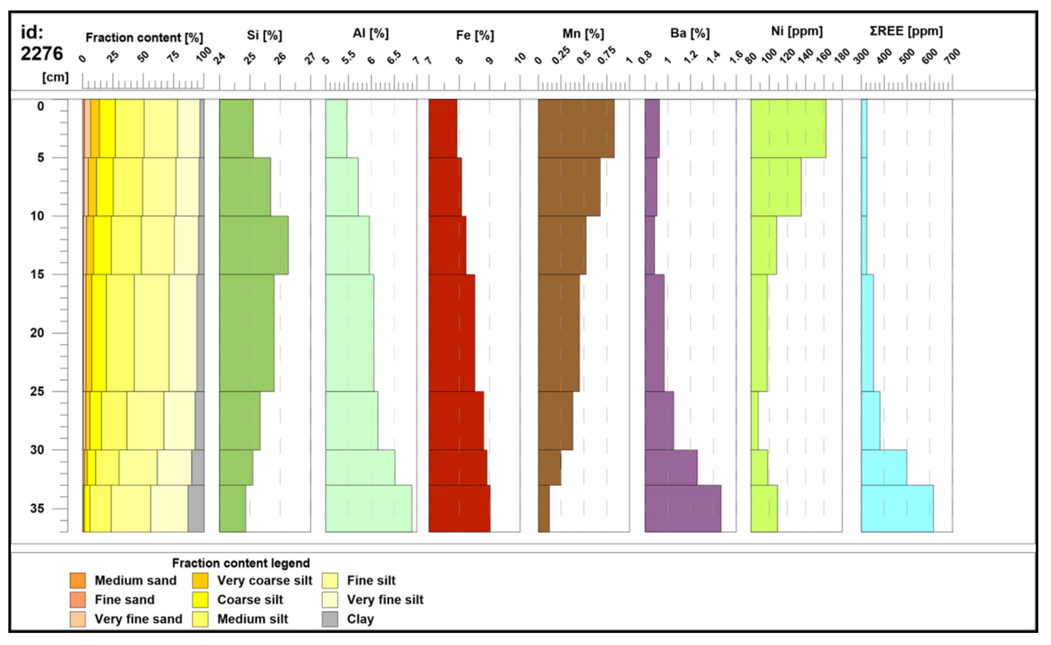
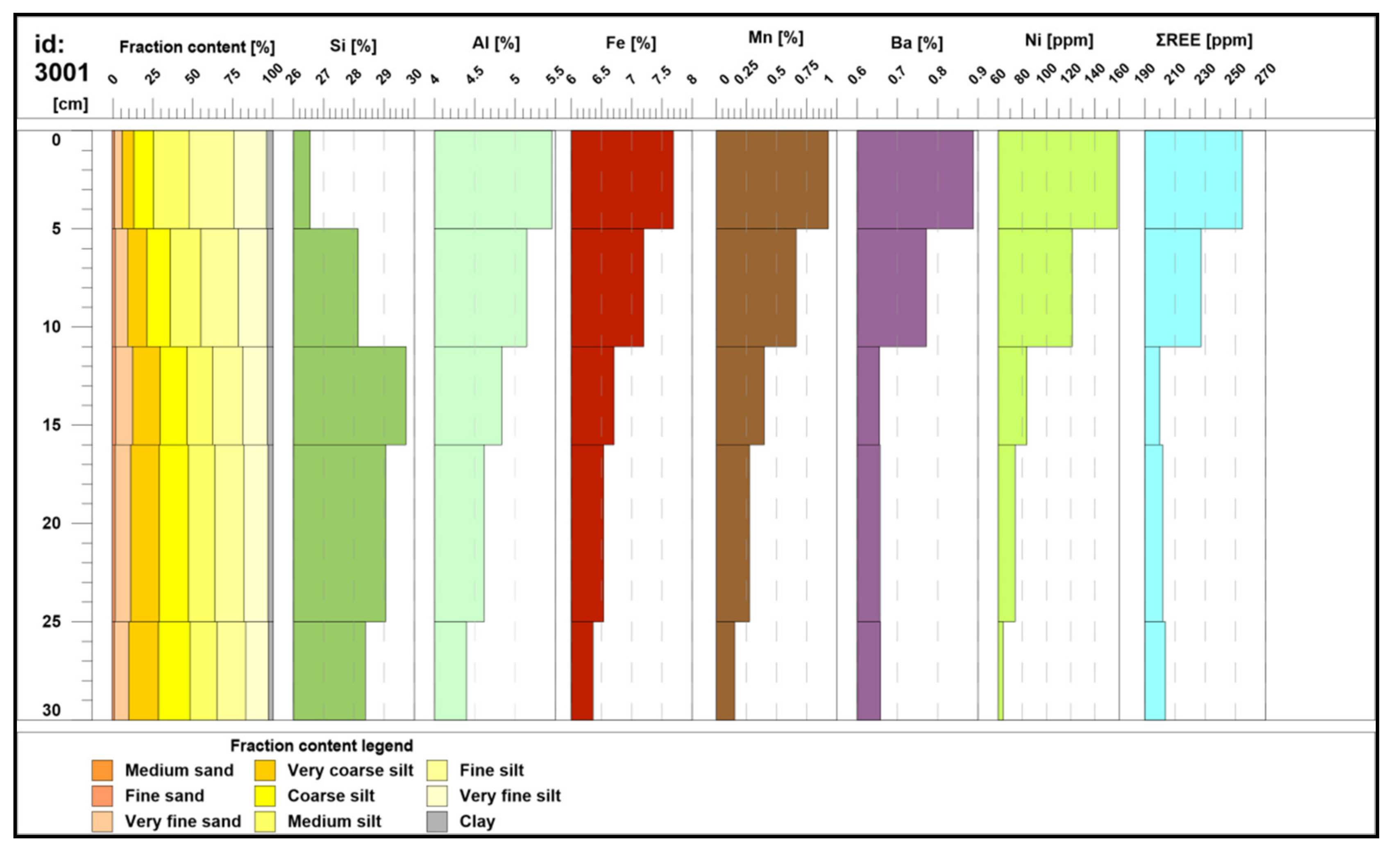
4.3. Geochemistry of Major Components, Trace Metals, and Biogenic Elements

All data of the major, minor, and biogenic elements is shown in Table S2. As shown by the EDXRF analysis of major elements, concentrations of Si and Al in all samples varied from 19% to 29.7%, and 4% to 6%, respectively. The highest contents of Si and Al were observed in horizon B. The mean content of both elements was respectively 23% and 5.3%, and was significantly lower in horizon C, mostly due to the dissolution of organic silica and transformation of clay minerals.
Concentrations of alkali metals (Na, K) were quite low (mean value 2.8%), ranging from 1.4% to 2.6%, and 2.6% to 3.2%, respectively. Potassium content was significantly lower in horizon C (x = 1.9%). The alkaline earth metal concentrations (Mg, Ca) were uniform, with a mean of 1.4% in both cases. A slight increase of Ca was observed in horizon C. The mean Ti content varied from 0.34% to 0.54%. The Cl content, due to diagenetic removal by halite crystallization, was lowest in horizon C. Contents of biogenic-associated P were lowest in horizon A (0.05% to 0.1%), and significantly increased deeper in the sediment column, with mean values of 0.64% and 0.84% for horizons B and C, respectively.
The AAS results show that Fe did not demonstrate important vertical differentiation. In horizons A, B, and C, mean iron concentrations reached 4.01%, 4.18%, and 4.02%, respectively. The Mn content was usually between 0.3% and 0.5%, with Mn/Fe ratios respectively of 0.12, 0.08, and 0.07.
The CNS analyses yielded low concentrations of carbon, nitrogen, and sulfur, which usually decreased with depth. The C content varied from 0.21% to 2.12%, with a mean of 0.55%. The N content was usually <0.1%, slightly decreasing with depth. The S content ranged from 0.33% to 0.70%, and was rather stable for all horizons. Mean values of C:N:S:P ratios were 5.4:0.2:6.6 in horizon A, 5.0:0.2:0.8 in horizon B, and 7.4:0.2:0.6 in horizon C.
A comparison of major and biogenic elements is presented in Figure 6.
Visible vertical and horizontal differentiation of several trace-metal contents occurred (Figure 7). The ranges of selected metal concentrations in all studied samples are as follows: 197−1173 ppm for Cu, 49−485 ppm for Ni, 17−277 ppm for Co, and 93−199 ppm for Zn. The Cu content in horizon A varied from 226 to 455 ppm, with a mean of 364 ppm. The Ni content varied from 65 to 348, with a mean of 171 ppm. Co ranged from 31 to 78, with a mean of 63 ppm. Ba concentration in the semiliquid geochemically active surface layer varied from 6120 to 11,730 ppm, with a mean of 9128 ppm.
Horizon B was characterized by broader ranges of all metals, with higher maximum and mean values. The Cu content varied from 207 to 1048 ppm, with a mean of 334 ppm. The Ni content varied from 65 to 485 ppm, with a mean of 127 ppm. The Co ranged from 25 to 165 ppm, with a mean of 54 ppm. Noteworthy are the highest concentrations of Ba, with a range from 5197 to 24,045 ppm and a mean of 8908 ppm.
The Cu concentration in horizon C varied from 197 to 1173 ppm, with a mean of 301 ppm. The Ni content ranged from 49 to 467 ppm, with a mean of 80 ppm. The Co content ranged from 17 to 277 ppm, with a mean of 43 ppm. The Ba content was similar to that of horizon A, ranging from 6170 to 13,645 ppm, with a mean of 8217 ppm.
Mean concentrations of Zn and Pb were quite stable within the sediment profile, and ranged from 93 to 199 ppm and 13–52 ppm, respectively. The Zn/Cd ratio increased from 590 in horizon A to 1609 in horizon C. The mean Sr and Rb concentrations were almost equal in all horizons, ranging from 348 to 353 ppm, and from 80 to 83 ppm, respectively. The Sc contents varied over 16–31 ppm. The highest Cr content occurred in horizon A (up to 627 ppm), and the lowest in horizon B (10 ppm).
The Mo content was characterized by a coefficient of variation as high as 270% (for horizon C). The highest Mo variability occurred in horizons B and C, respectively, by coefficients of variation as high as 219% and 145%, as well as by Ca (89%) over horizon C, and Ni (73%) over horizon B. The smallest variabilities are typical for Ti (2%), K (3%), Al (4.5%), Cl (5%), and Mg (9%), as observed in horizon A. The Th and U contents were also low and varied over 7.0−12.3 ppm and 1.0−1.9 ppm, respectively. The Th/U ratio was from 6.15 to 6.54, and usually increased with depth. The mean Cu:Ni:Co ratios were 2.1:2.7 in horizon A, 2.6:2.3 in horizon B, and 3.7:1.8 in horizon C.

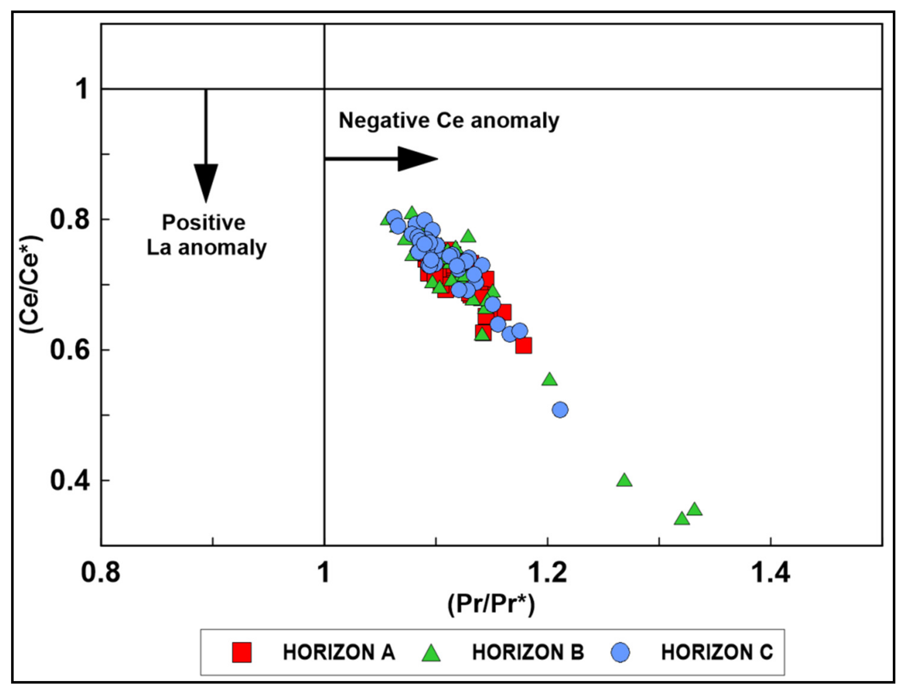
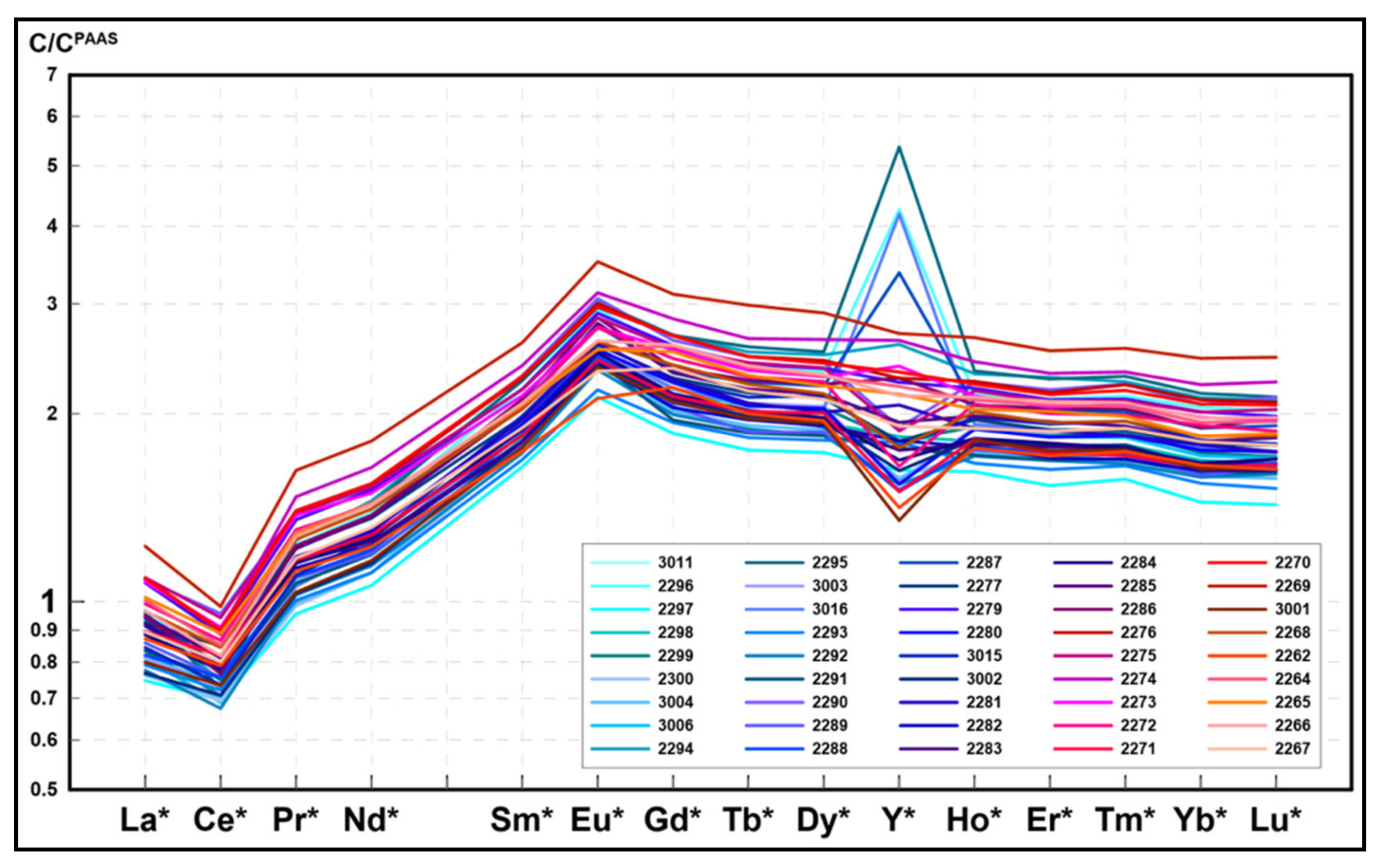
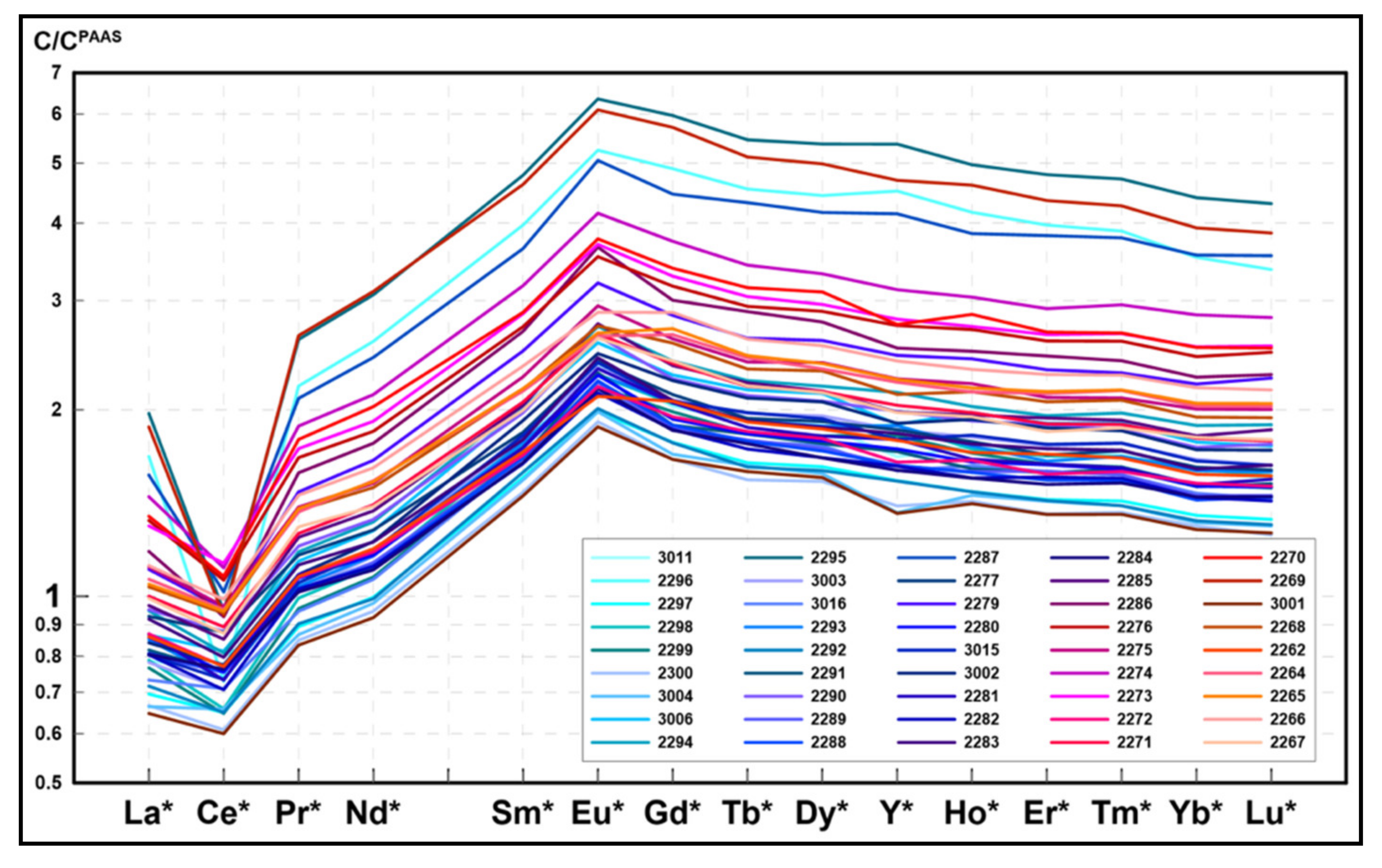
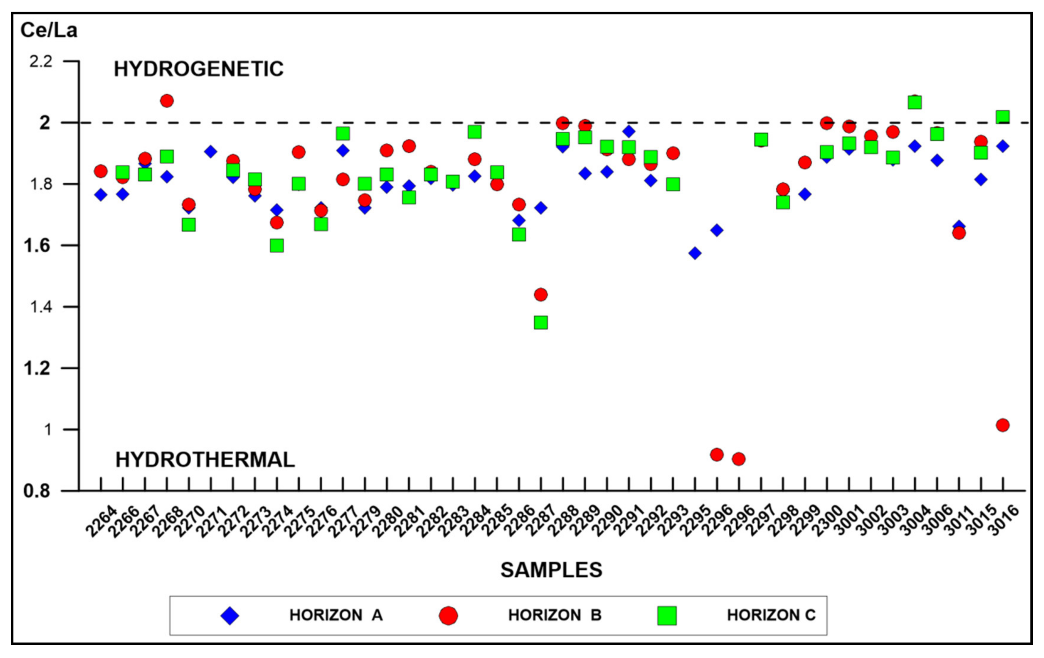
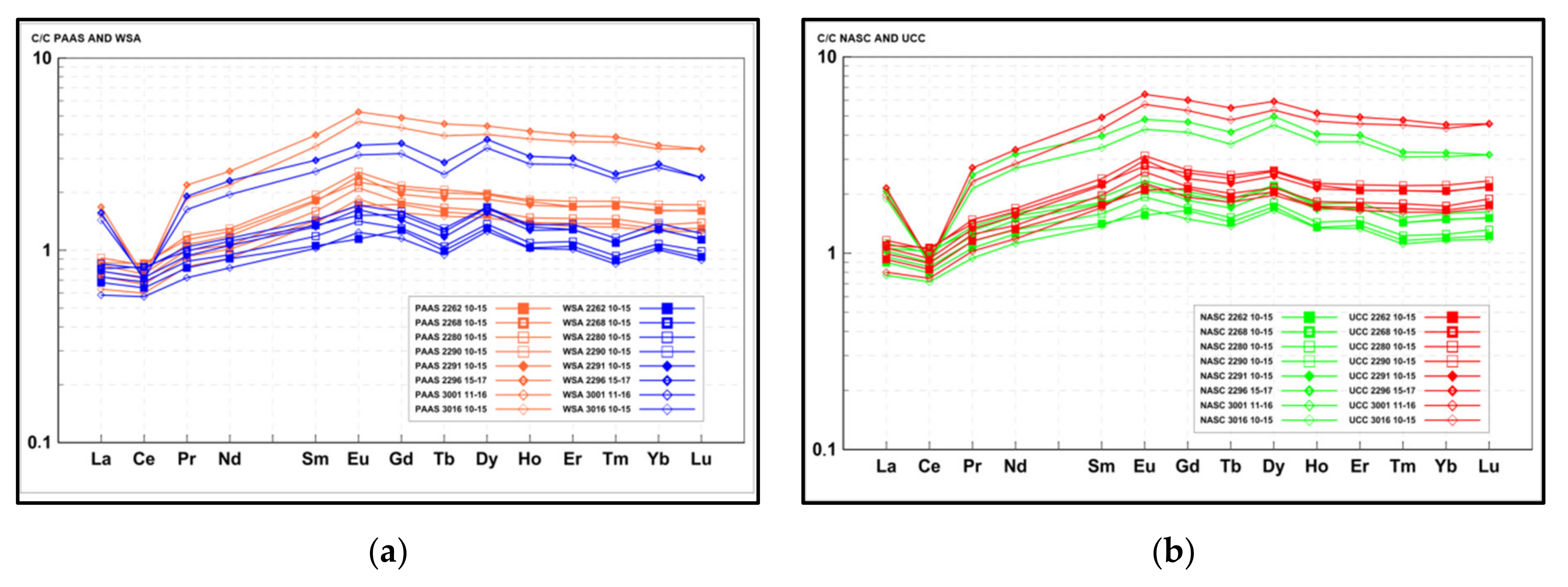
4.4. Rare Earh Elements
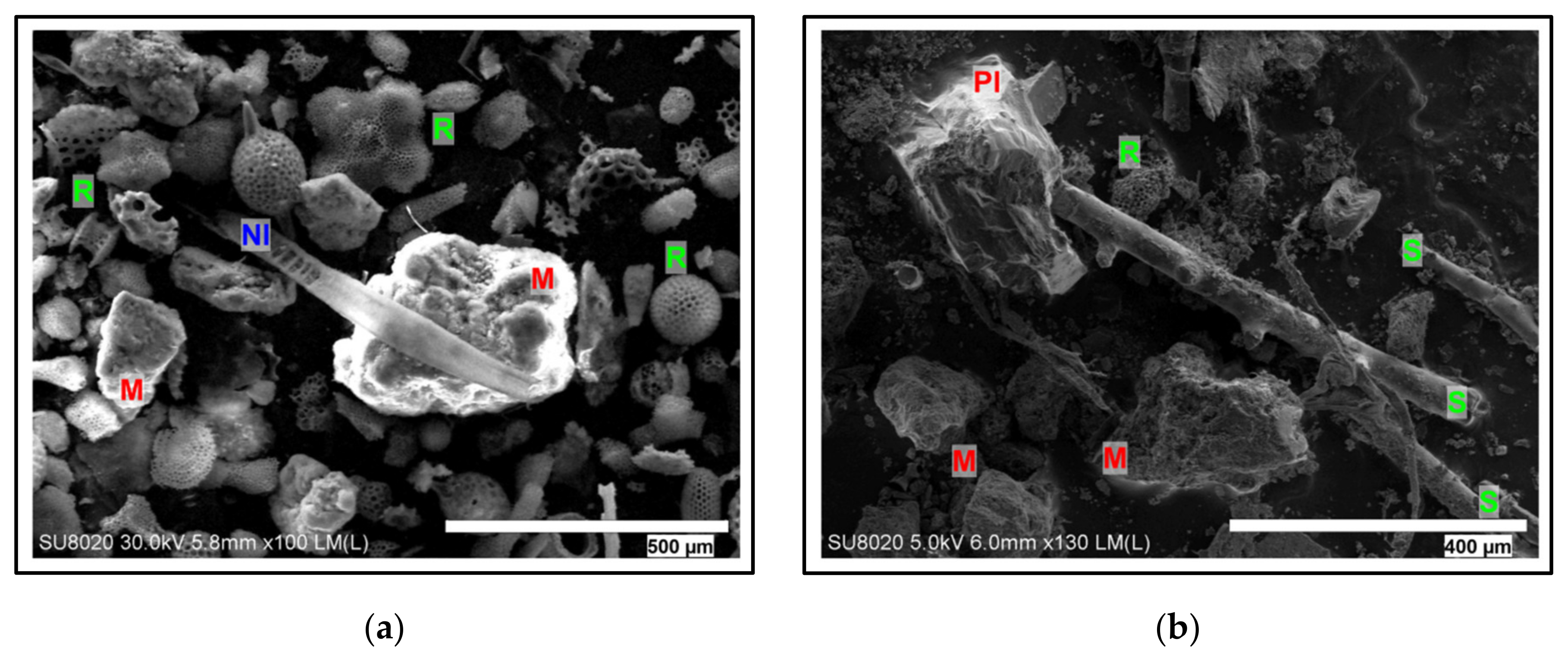
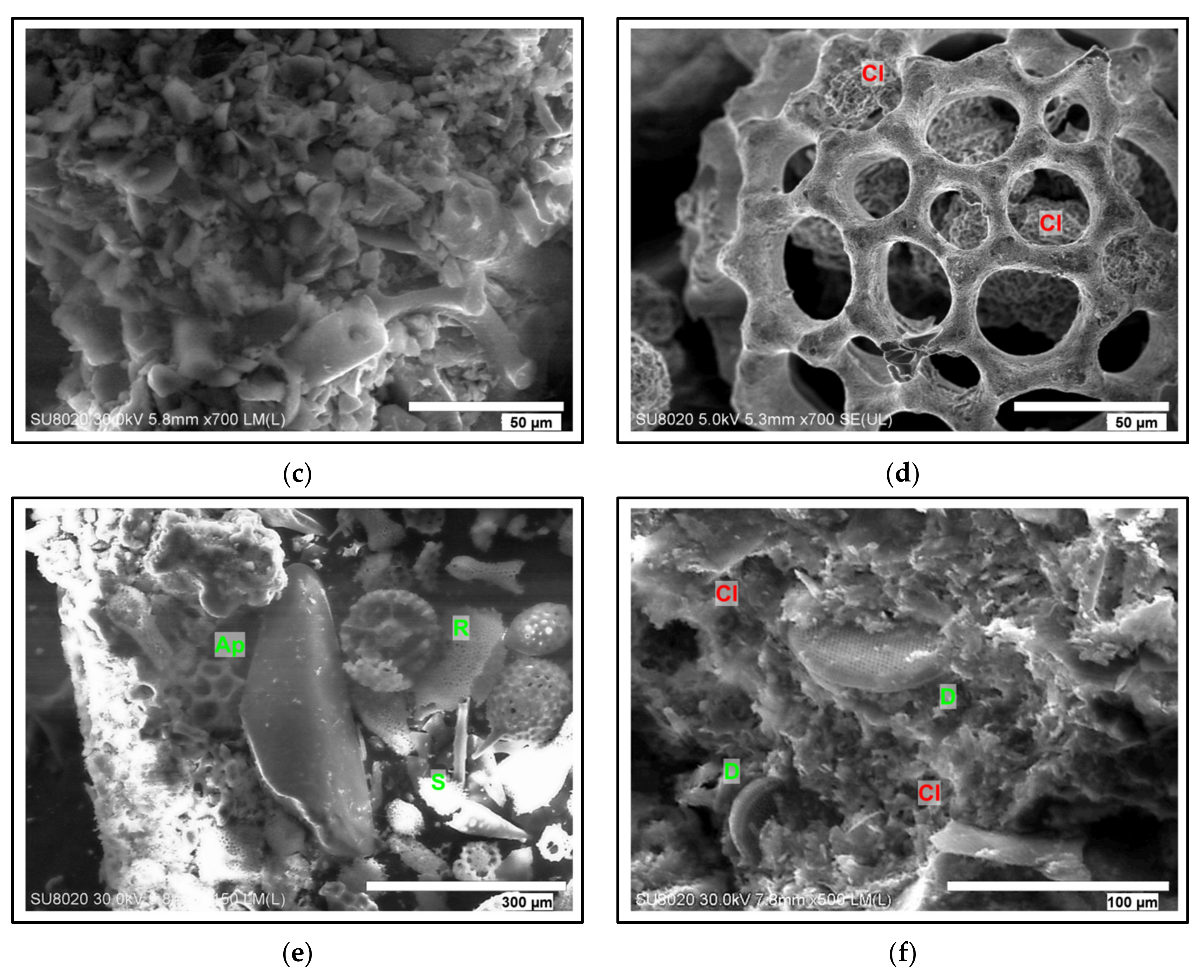
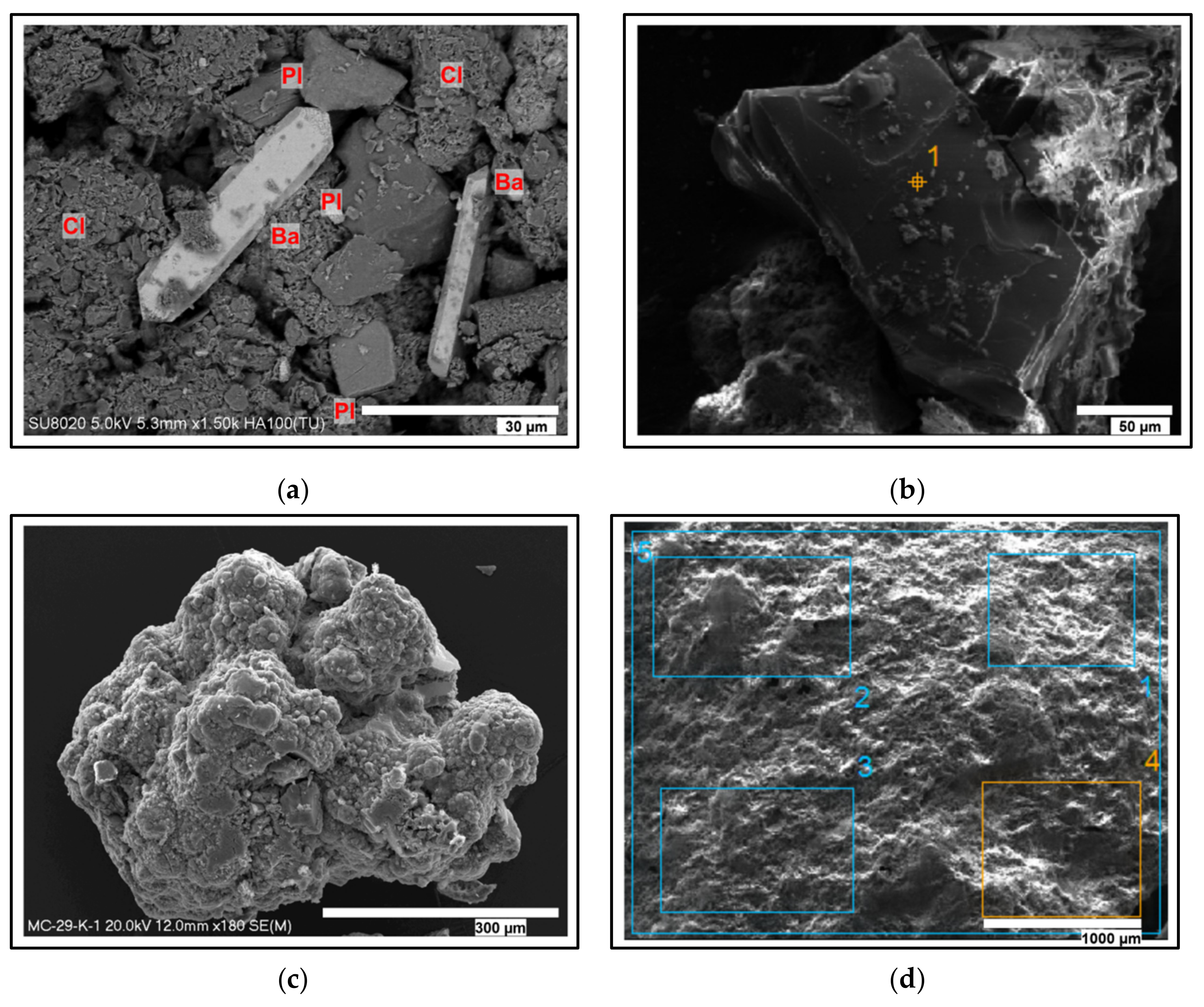
As shown by the ICP-MS, total REE content varied from 200 ppm to 577 ppm, with a mean of 285 ppm (Figure 7). The total light rare elements (ΣLREE) content ranged from 127 ppm to 339 ppm, with a mean of 182 ppm. Total heavy rare earth elements (ΣHREE) concentration ranged from 23 ppm to 83 ppm, with a mean of 33 ppm. The highest mean contents of ΣREE, as well as ΣLREE, for horizon C were 291 and 187 ppm, respectively. In this horizon, REE were dominated by Ce, Y, Nd, and La (with means of 66, 56, 47, and 37 ppm, respectively). The highest ΣREE content variability, expressed by the coefficient of variation, occurred in horizon C (26%), and the lowest in horizon A (10%).
The highest mean content of ΣHREE occurred in horizons B and C (both 83 ppm). PAAS-normalized REE distributions were similar for each horizon and showed negative Cean (0.36−0.81), weakly positive Euan (1.07–1.30), noticeable enrichment of MREE in comparison to LREE, and a slight depletion of HREE in comparison with LREE (LREE/HREE in the range of 0.53–0.69) (Figure 8, Figure 9 and Figure 10).
There was no significant difference in PAAS-normalized REE distributions among horizon A samples. Negative Cean varied in the range of 0.61−0.78, with a mean of 0.71, while positive Euan values ranged from 1.07–1.29, with a mean of 1.22. The YSN/HoSN ratio, which represents the decoupling of geochemical twins Y and Ho, and is a quantitative image of Yan in REE patterns, varied from 0.95 to 1.10, with a mean of 1.02. The significant enrichment of MREE compared with LREE can be seen in the spider diagram (Figure 8).
Higher diversity in PAAS-normalized REE distributions occurred in horizon B, where several samples showed strong positive Yan, expressed by YSN/HoSN ratio higher than 1 (max. 1.11), while other samples showed slight negative Yan (YSN/HoSN < 1). A few peaks of Yan are clearly visible in the spider diagram (Figure 9), which show positive Yan that may be related to increased contents of bioapatite, zeolites, or plagioclases. Negative Cean in horizon B indicates a wide range, and varied from 0.36 to 0.81, with a mean of 0.71.
High variation in PAAS-normalized REE distributions also occurred in horizon C, which had the highest range of ΣHREE (203−544 ppm). Negative Cean in this horizon was also of wide range, varying from 0.67 to 0.80, with a mean of 0.72. Samples showed both negative (YSN/HoSN = 0.94) and positive Yan (YSN/HoSN up to 1.09). A slight depletion of HREE, as compared with LREE (LREE/HREE in range of 0.56–0.69), was also observed (Figure 10).

4.5. SEM-EDX

The SEM-EDX analysis confirmed the presence of the components found by XRD analysis, including detrital minerals such as quartz, plagioclase, pyroxenes, as well as diagenetic barite, and micronodules, small amounts of volcanic glass, and nonidentified lithoclasts (Table S3). Zeolites and calcite were not confirmed. Among the biogenic components, the biogenic skeletal remnants of radiolarians, sponges, and diatoms were identified. Foraminifera, mostly agglutinated and rare calcium carbonate, as well as phosphate remnants (carbonate-fluorapatite—CFA) occur in the form of fish teeth or skeletal debris (Figure 11a–f).
The increased barium content in all horizons was associated with barite (BaSO4). Diagenetic barite crystals occurred in the form of elongated coffin-shaped euhedral crystals, with dimensions that varied 20 to 100 μm (Figure 12a). Analysis by EDX revealed low substitution of Ba by Sr (up to 1.5%). Chemical impurities also include Si (1.3%), Fe (0.5%), Ca (0.1%), and K (0.1%).
Plagioclase signatures are typical of volcanic debris (Figure 12b). Domination by Ca and Na suggests the presence of bytownite-andesine-oligoclase endmembers. Additionally, in the feldspar debris, traces of Y (up to 200 ppm, not presented in this paper), Cr, Ti, and metals such as Cu and Ni were identified.
The examined micronodules were small Mn–Fe particles, usually <2 mm in diameter, formed in sediments by complex diagenetic-hydrogenic processes, which showed increased contents of metals, such as Ni, Cu, Co or REE (Figure 12c,d). The weight amount of micronodules in the selected sediment horizons may reach a few percent [84,85]. Micronodules showed high levels of Mn, with a mean content of 50.8%. The mean content of Fe was 13.5%, while for Ni + Cu, it was 3.0%, and in some cases, exceeded 5%. Micronodules showed admixtures of external components, mostly debris or clay aggregates, rich in Si and Al, totaling 8–9%. Additionally, micronodules showed increased Zn contents and traces of Ti, Na, Ca, Mg, K, Ba, Sr, Mo, Sc, and F. The level of phosphatisation was low, usually <0.1%. The contents of S and Cl were also low.
According to some geochemical signatures (Figure 13), micronodules from IOM H11 were formed by a diagenetic influx of hydrogenic processes (so called mixed-type). The complete SEM-EDX geochemical data for micronodules are presented in Table S3.
Biogenic phosphates were represented by carbonate fluorapatite (CFA), which contained impurities of metals such as Ni or Zn, usually around 3–4%. Additionally, increased contents of S, Cl, and F were identified. The CFA may show elevated contents of REE, dominated by Y and La, which may reach more than 0.5%. Analyzed fish remnants showed traces of Fe, Mn, Si, Al, Cr, Ti, alkali, and alkaline metals.
The clay dominated separates showed a Si/Al ratio of 2.3–2.4 and elevated contents of Fe, with minor quantities of Mn, Cr, Ti, Ba, and Ca. The mean contents of Na, Mg, and K were 3.2%, 2.4%, and 1.9%, respectively. The Cl content was also increased, mostly by interstitial halite crystallization, reaching from 1.5% to 2.0%.

4.6. Correlations

4.6.1. Horizon A

The grain size of the active layer (horizon A) was dominated mostly by fine silt and clay subfractions. The REE (apart from Ce), P, As, and Co showed low positive correlation coefficients (0.42–0.51) with medium silt. The Fe and Mn showed strong positive correlation (0.93), but were correlated negatively with P (−0.68 and −0.73, respectively), Pb, Mo, Ba, and REE. The highest positive correlations of Mn were found with Sn and Sc. Mn was better correlated with C and N, compared with Fe. Iron showed good correlation with clay minerals, especially chlorite, confirming Fe-rich types of minerals (nontronite and Fe-chlorite). Phosphorus showed good positive correlations with REE (0.48–0.50) and Pb. P was also positively related to allogenic mineral components, such as quartz, pyroxenes and kaolinite, or diagenetic barite. Metals such as Cu, Ni, Co, Zn, Pb, Mo, Cd, Sb, Sn, Sr, and Rb usually showed positive correlations with each other (0.45–0.75). Ag, Cd, Tl, and Cr showed no positive correlations with other metals, or weak negative relations (−0.2 to −0.3). Metals showed positive correlations with REE, usually around 0.4 to 0.7. Ba was positively correlated with Pb, Th, and biogenic elements (C and N; 0.55 and 0.78, respectively). Sc showed similar behavior to other REE, correlating positively with barite, clay, quartz, and plagioclase contents.
The REE positively correlated (>0.9) with total clay minerals content (0.5), and with detrital minerals, such as quartz or feldspar. Ce showed slightly anomalous behavior, i.e., lower positive correlations with metals and other REE (0.6 to 0.7). REE did not correlate with Fe and Mn, and showed a negative relation with halite and amorphous silica content (0.5 to 0.7, respectively). The C and N also showed negative correlations with REE, but was positively related to S.

4.6.2. Horizon B

Similar to with horizon A, the grain size composition of horizon B was strongly related to the quantity of fine silt and clay fractions (0.86–0.93). REE content was essentially positively correlated with fine fractions, clay minerals, barite, and metals such as Fe, Mn, P, Ba, and S. Ce showed positive correlation only with P (0.66), Zn, Pb, As, Sn, Rb and Sc. Similar behavior occurred with Sc, which was more strongly related to U and Th, than Ce. Fe and Mn were positively correlated (0.94) and also showed positive relations with other metals (0.6 to 0.9) (Figure S1). Anomalous behavior (lack or low correlations) was indicated with Ag, Sn, Rb, Sc, and Ce. Correlations between Ni, Cu, and Co were high (0.9>). Mn and Fe showed strong positive correlation with Sr, Ba, and S (around 0.6 to 0.9). Metals such as Ni, Cu, Co, Zn, Pb, As, Mo, Cd, Tl, Sr, and Ba showed positive relations with each other, i.e., usually around 0.7 to 0.9, but did not show positive correlations with Rb, Ag, Sn, and Cr. Th and U contents showed positive correlations with P, Zn, Pb, As, and Sn (0.5–0.7), as well as with REE (0.4–0.5). Biogenic elements such as C and N indicated strong negative correlations with fine fractions, metals, and REE (−0.5 to −0.9). Different behavior was displayed by S, which showed positive relations with fine fractions and most metals, including REE.
Compared to active layer, correlations between minerals and selected elements were clearly visible. The feldspar content was positively related to clay minerals (especially smectite) and barite (0.6–0.9). Barite was positively correlated with REE. Kaolinite and illite did not show any special relations with REE and metal contents, apart from P, Rb, Sc, Ce, Th, and U. Biogenic amorphous silica was positively correlated with coarser fractions, biogenic elements (C and N), and halite. Opaline silica showed strong negative relations with almost all metals.

4.6.3. Horizon C

The correlations between selected metals and minerals in horizon C were comparable to those in horizon B, but more uniform and distinctive. The REE were positively correlated with fine fractions (0.6–0.7). Correlations of metals (excluding Cr) with coarse fractions were significantly more negative, compared with the two higher horizons. Almost all metals showed positive relations with Fe and Mn. Additionally, P, S, and REE showed strong positive correlations with most strategic metals, except for Ag, Sn, and Cr. The REE correlation with S was also weaker in comparison with horizon B (0.26–0.33). P and most metals (apart from As, Ag, Sn, Rb and Th) were well correlated with each other (>0.8). P was strictly related to fine fractions, while correlating negatively with Cr, C, and S. Ba and Sr showed similar behavior. The contents of Th and U also showed positive relations with Ag, As, Sn, Rb, as well as with fine fractions, especially fine silt and clay. C and N indicated negative correlations with all metals, and correlated positively only to coarser fractions.
For minerals, barite was positively correlated to other metals and REE (0.8–0.9); however, a lower coefficient was observed in the case of Ce (0.7). Feldspars were positively correlated to clays, especially smectite and illite, and additionally to REE.
According to the comparison of grouped LREE-MREE-HREE correlation coefficients in horizon A, there was a general tendency for correlation increase between HREE and coarse fractions, as well as P contents. The ∑REE content seemed to better correlate with Mn than Fe. In horizon B, the relation of ∑REE with P was less significant, and appeared to be more uniform in each subgroup. The REE showed stronger relations with Fe than Mn. In horizon C, the picture is quite similar; however, a slight increase of correlation coefficient between ∑REE, P, Ba, and clays was observed. The full correlation coefficients matrices for each sampling horizon are presented in Figure S1.

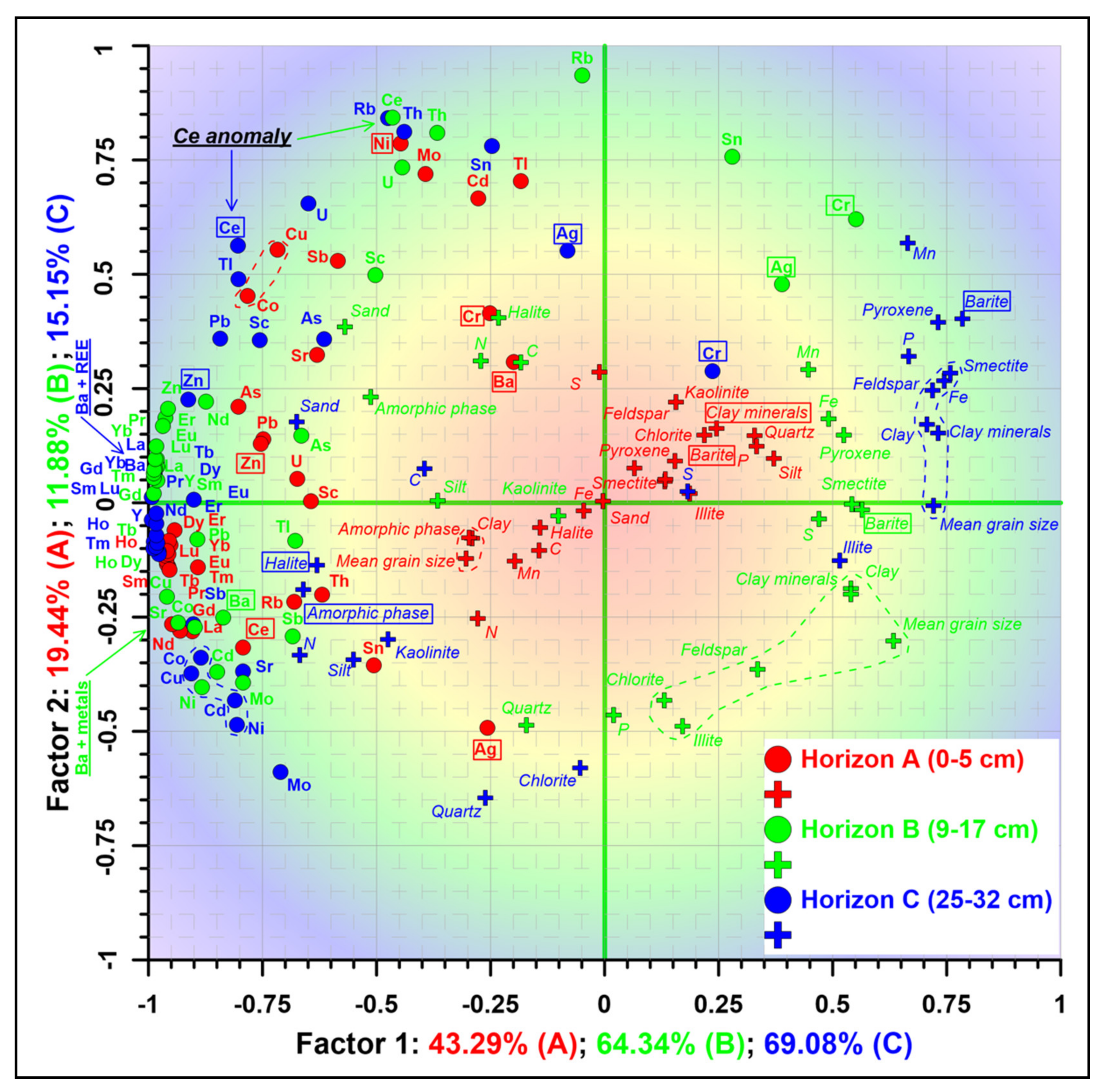
4.7. Principal Components Analysis (PCA)

The FA and PCA analyses indicated a dominance of two factors (components), which covered 63%, 76%, and 84% of the total analyzed sample variability in horizons A, B, and C, respectively. The influence of factor 1 increased gradually in horizons B and C (64% and 69%, respectively). The value of factor 2 was quite uniform for all horizons, but showed an increase from the top to the bottom sections of the sediments. Other minor factors were also uniform in all horizons (Figure 14).
The PCA loadings showed a strong fractionation of REE and selected metals in horizon A. Most other variables were dispersed on the PCA loading plot (Figure 15), indicating low correlations. REE and metals such as Sn, Rb, Ag, and Th showed negative correspondence with Mn, Fe, amorphous silica, halite, C, N, and clay fraction, when compared with other metals (i.e., Ni, Cu, or Co). These patterns may suggest an external REE source, controlled mostly by biogenic input, coarser fractions (mostly silt), and relations with polymetallic nodule formation mechanisms. Critical metals showed weak positive relations to coarse fractions, illite, and quartz content, which also suggest dominance of external factors (hydrogenic or hydrothermal input).
Variables in horizon B showed different behavior and grouping of REE, or several other metals. The REE, apart from Ce and Sc, were positively correlated with other metals such as Fe and Mn, as well as clay minerals (especially smectite) or barite, which suggests diagenetic remobilization. The relation was negative with amorphous silica content, biogenic elements (C, N, and P), silt, and sand fractions. Ce, U, and Th are grouped in a second small cluster, suggesting some different oxidative behavior, or a relationship with biogenic phosphates input and dissolution. The visible grouping of variables and the unification of factors are related to more pronounced fractionation in comparison with horizon A.
Variables in horizon C showed behavior similar to horizon B, and even more apparent REE and metal groupings, which may be related to Fe and Mn immobilization, barite formation, or to decomposition of phosphates. The relations were also positive with some external components, such as plagioclase or pyroxene contents, suggesting additional external influences. Fractionation model in horizon C may be strongly shaped by a diagenetic transformation of clay minerals, burial degradation of allogenic components, or barite formation, mostly in regime of extensive S and P suboxic consumption.
The anomalous Ce positions in the plot may be related to different oxidation properties of Ce3+. Even such an autonomous metal as Ag (besides Cr) is fractionated in horizon C, indicating a strong relationship with the transformation processes that occur in sediments.

4.8. Spatial Variability

The sedimentological, geochemical, and mineralogical data presented on the maps show distinctive spatial features (Figure S2).
The mean grain size of siliceous clayey silts shows generally highest variability in the E–W direction, and lowest in N–S. The sediments show patchy-like type of zonality. The spots of coarser material were located in the central part of the study area, and in case of horizon A, also in the NE part of the polygon. The finest sediments were located mostly in the outer parts of IOM H11, especially western and eastern portions of the region. The pattern was generally the same in all horizons; however, at greater depths, it was most uniform in horizon C.
The total content of Cu, Ni, and Co showed spatial features other than grain size. The data generally trended NW–SE, with the lowest variability being observed in the SW–NE direction. The metal contents were more evenly distributed in the active layer in comparison with horizons B and C, and did not show any specific trend. In the active layer, the highest concentrations were observed in the SW and NE parts of the polygon. The lowest values occurred in the central study area.
Compared to the active layer A, horizon B showed the lowest content of metals in the NW and SE of polygon. The zone of intermediate metal contents was oriented N–S, with a few spots of increased content in the NE area. The mean contents of metals in horizon B were generally lower compared to the active layer, but higher than in horizon C.
The total metal content in horizon C generally trended NW–SE. The lowest contents occurred in the central and SE parts of the polygon, increasing towards NW with a few concentrations of higher metal contents being observed in NW area. The total metal contents in horizon C were lower in comparison with horizons A and B.
The ∑REE distribution maps show good spatial convergence with grain size and SiO2am/clay minerals ratio, especially in horizons B and C. The REE data trends were similar in horizons B and C. The highest variability occurred in the NW–SE direction. The elevated contents of REE in the active layer occurred in NW and N parts of the polygon. Horizon B and C showed similar distributional patterns, and the intermediate REE content zonation was oriented N–S, which mostly covered the central part of the polygon. Elevated contents of REE occurred in some concentrations located near the eastern border (horizon B) and western part of the region (horizon C) of IOM H11 polygon.
The maps of amorphous silica/clay minerals contents show the influences related to diagenetic burial dissolution of silica and transformation to clay minerals. The highest ratios of both variables show NW–SE trending in all horizons, with the lowest ratios in the eastern and western parts of the polygon.
The lithological profiles presented in Figure 16 show vertical changes of the grain size composition, mineralogy, and geochemistry of individual horizons A, B, and C (Figure 16, Figure 17 and Figure 18). Three general models of vertical variability were observed: (i) the content of REE, Fe, Al, Ba, and clays was intermediate and increased with depth, while the amount of Si, Mn, Ni (and other metals), and coarse grain fraction decreased or was uniform in all profiles (Figure 16); (ii) the content of REE, Fe, Mn, Al, Ni (and other metals), and Ba was lowest among all samples, while coarse fraction content was the highest in horizon A, and the Si (and amorphous silica) content increased with depth, or was quite uniform (similar to clay minerals) (Figure 17); (iii) the contents of REE, Fe, Mn, Ni, and Ba were highest in all sample populations and associated mostly with horizon B, while Al, Si, and clay contents increased with depth or were quite uniform within the profile (Figure 18).

5. Discussion

The sediment distribution and composition in CCFZ depends on several environmental factors, including:
  • moderate biological productivity of surface waters (higher in the eastern area and lower in the west);
  • bathymetry and distinctive linear topography of the seafloor;
  • low sedimentation rates;
  • depth of CCD ranges from 4000 to 4500 m, which determines CaCO3 contents <10%;
  • early diagenesis processes affecting neoformation and transformation of clay minerals;
  • tectonic, volcanic and seismic activity [43].
Surface sediments from the IOM H11 area show significant spatial relationships to the accumulation of REE and other strategic metals. The main process that influences scavenging of rare earths is the early diagenetic remobilization of metals and neoformation of diagenetic clay minerals. Acquisition of REE is related to sorption and immobilization mechanisms during the transition from oxic to suboxic conditions. The formation of Mn–(Fe) oxyhydroxides as micronodules and clay minerals, mostly Fe-rich smectite, determine the bonding of REE and metals, such as Ni, Cu, or Co. Other processes of different REE fractionation patterns include: (i) the presence of allogenic biogenic phosphates, mostly CFA, in the form of teeth and skeletal remnants of fish, which may determine low Cean indicated in selected samples; (ii) admixtures of detrital material, such as feldspars or pyroxenes, which may explain the higher metal contents in some sample locations, or increased contents of HREE; (iii) the presence of micronodules or nodule remnants, which usually show greater quantities of REE and other metals, in comparison with sediments.
The data of mean grain size and total Cu, Ni, and Co contents showed low spatial correlation in the active layer (horizon A). The highest metal contents correlated with finest fractions, especially in SW and E of study area. The spatial relations between SiO2am clay minerals were not so clearly apparent; however, the lowest ratios, related to increasing clay contents, corresponded positively with the highest metal contents in the active layer. Some anomalous spots, including sample stations 2262 or 2292, showed the presence of higher micronodule quantities, which are visible in grain size data, as medium or fine sand subfractions.
The zonation of REE and metal contents in horizons B and C were similar, which may constitute evidence of the same fractionation trends. The lowest contents of REE were observed in the central and S part of polygon, excluding only few stations, such as 2264 or 2295, where increased REE contents also occurred within sediments with intermediate or elevated amounts of Cu, Ni, and Co. These patterns indicate REE fractionation between coarser fractions of sediments, to suggest that low contents of biogenic silica are needed to accumulate REE. These processes may correspond with early diagenetic remobilization of metals in horizon B, or REE and metal scavenging controlled by clay minerals adsorption. Described remobilization patterns may be strongly conditioned by biogeochemical processes within the sediment column, related to burial and reduction of sulphates and organic carbon degradation, likely controlled in some cases by bacterial processes, denitrification, and finally, the dissolution of biogenic phosphates, mostly CFA [87].
The distribution patterns of total metal content and REE were similar in horizons B and C, but were different in the active layer. The highest contents of REE occurred in the NW part of the polygon, accompanied by elevated contents of ∑Cu, Ni, and Co. The strong evidence of diagenetic fractionation of metals and REE corresponds well with fine silt and clay subfractions, which dominated in the NW part of polygon. The pattern of diagenetic REE uptake is particularly apparent in horizons B and C, when compared using the REE distribution map with SiO2am/clay ratio. The increased influence between metals accumulation (including REE) and clay fraction contents, or lesser contents of silica, is especially apparent when horizon C is compared with A. Horizon B is a transition between A and C, where the described parameters were in the middle, suggesting some stability or gradual change of diagenetic processes in the uppermost 30 cm of sediment column.
A comparison of grain size data showed that quantities of clay minerals, biogenic silica contents, and REE distributional patterns, as well as the early diagenetic immobilization of metals such as REE, Ni, Cu, Co, or Zn, could also be related to the presence of micronodules. In the lower sediment depths, the feldspars content showed a positive relationship with clay minerals, especially illite and smectite, which may be an indicator of burial alteration and plagioclase decomposition processes [88]. REE related to feldspars or other allogenic debris components may be an additional source of Y or HREE, mostly in the deeper parts of sediment column. Additionally, in horizon C (or even deeper), the role of P, S, and Ba in the acquisition and fractionation of REE increased.
The observed REE ratios are important indicators of hydrogenic, hydrothermal, and biogenic processes. The Ce/La ratio is an indicator of the relationship between hydrogenic (>2) and hydrothermal (<2) impact upon sediments [9]. In that study, Ce/La ratio ranged from 0.9 to 2.07 (Figure 19), with only seven samples reaching or exceeding a value of 2, accompanied with positive Euan. These suggest a strong positive relationship between sediments and hydrothermal conditions. Pelagic sediments are usually Ce depleted and show a negative Cean, while polymetallic nodules usually indicate strong positive Cean [6]. This factor, as well as enrichment of MREE compared to LREE and HREE, is typical for sediments formed away from terrigenous sources at relatively slow sedimentation rates [4].
The REE fractionation in oceanic waters was reflected in the mineralogical and geochemical composition of bottom sediments. The REE content and positive Cean usually increases in sedimentary processes, with a higher contribution of reactive iron and manganese. Increase of bone debris content in pelagic clays, as a result of low sedimentation rates, leads to the inversion of REE composition. The depletion of Ce and LREE becomes stronger, mainly because bone debris accumulates considerable amounts of REE dissolved in oceanic water, probably without any noticeable fractionation. Pelagic clay with high bone debris content represents the terminal member in the series of sediment types formed during the oceanic material fractionation [4]. Negative Cean were related to the different oxidation potential of Ce and were associated strong relation with Mn–Fe oxyhydroxides, which are the main oxidizing agent [56].
Oliver and Boyet [89] suggested that Cean, as well as the enrichment of HREE relative to LREE, could be masked due to elevated contents of terrigenous material. This situation is particularly true, as regards the clay minerals and fine grain quartz, often depleted together with REE [90,91]. Bau and Dulski [92] proposed a binary diagram, which provides a test of whether the calculated negative Cean was real, or masked by positive Laan (Figure 20). Low Gdan, apparent in a few samples, was likely related to inorganic speciation, as well the positive Euan, which is usually connected with hydrothermal input [56].
The issue of normalizing the REE results to individual rock standards was broadly discussed by [6]. The most commonly used standards are the North American Shale Composite (NASC), Post Archean Australian Shale (PAAS), Upper Continental Crust (UCC), World Shale Average (WSA), and chondrites; however, depending on the author, the values may differ. A less commonly used rock standard is clay from the Russian Platform [93].
A comparison of the REE distributions in the selected samples of horizon B normalized to different rock standards is presented in Figure 21. These samples were selected to show the most representative values (maximum and minimum REE contents, including LREE and HREE, or LREE/HREE).
There are several differences in normalized values, and in the shape of spider diagrams. The PAAS-normalized values were higher than WSA (the difference ranges from 4% for Ce to 58% in Tb), and spider diagrams are more flattened (Figure 21a). Positive Euan was higher (9.8%) when PAAS-normalized, but slight Tban and Tman are present on the WSA-normalized spider diagrams. In both cases, the distributions were enriched with MREE, in comparison to LREE. The NASC-normalized REE distribution diagram was similar to the UCC-normalized one; however, for all samples, positive Dyan are apparent on NASC-normalized diagrams (Figure 21b).
The most significant differences in values and shapes of spider diagrams are apparent with chondrites-normalized REE distribution (Figure 21c). The values were higher than other standards by two orders of magnitude, and the spider diagram trends are reversed, i.e., distributions are enriched with LREE, in comparison with MREE and HREE. The Cean were similar to other standards; however, only chondrite-normalized REE distributions showed slightly negative Euan, i.e., in the range of 0.78 to 0.92. The above comparison indicates the accuracy of the rock standard used to normalize the results of the analyzed sediment samples.
Observed negative Cean usually represent variability of oxic conditions into a sedimentary environment and in the water column, but in this particular case, the changes were caused mostly by authigenic phosphate and authigenic Fe-rich smectite formation, being the effect of early diagenesis. The reaction between Fe oxyhydroxides and biogenic opal, by which the Fe-smectite can be formed, suggests an early diagenetic process, which is in equilibrium with seawater REE [94]. Of particular note, the PCA indicated an increase of Ce geochemical independence with depth, especially apparent in horizon C, which may have been caused by the different oxidation behavior of Ce, compared to other REE. Ce showed similar trends to U or Sc, and did not correlate with metals, such as Ni, Cu, or Co. This shows that the accumulation tempo of these metals and REE differed significantly due to oxix-suboxic changes in the sediment column, caused mainly by early diagenetic processes.
The high quantity of Fe-smectite may indicate the primary presence of pyroclastic material, such as volcanic glass, and effect of halmyrolysis. This mineral may also have a detrital origin, but the quantity in the analyzed samples (6.6–32.8% of all mineral phases), the occurrence of volcanic glass previously found by [60], and the distance from land are suggestive of authigenic origin [95].
Since the depth of sampling sites ranged from 4333 to 4443 m, which is below CCD, the cause of increased calcite content in some samples (up to 9.2%) is not clear. There could be two reasons for calcite enrichment of these sediments: (i) as per quoted CCD depths in CCFZ [42], some sample stations in the eastern part of studied area may have been above or within the CCD interval (for example sample 2297 25-30, which contained the highest quantity of calcite, sampled from a depth of 4333 m); (ii) the carbonate-rich sediments could occur below CCD due to slumping. An increased concentration of calcite in the sediments below CCD was found also in the southern part of BGR Claim Area adjacent to IOM H11, explored by the Federal Institute for Geosciences and Natural Resources of Germany [96].
Local heterogeneity of geochemical parameters is related to small scale local variability of depositional environment parameters, such as topography, biological productivity, hydrothermal effects, dissolution of nodules, or redox zonation [97]. In some parts, the elevated metal contents in CCFZ may also be related to buried hydrothermal microchimneys [98].
Apart from this, admixtures of REE may be related to weathered basaltic material from the Hawaiian area seafloor [99]. The elevated REE concentrations can also be attributed to desorption from resuspended sediments and pore water released into the overlying water column [100].
Increased CaCO3 concentrations (maximum values at 19–28 cm bsf) can also be associated with abundant and well-preserved foraminifers, and may be correlated with the last glacial maximum (approx. 26,500–19,000 years ago) [101], when the increased productivity zone was located more to the north. At that time, the CCD interval was lower, associated with higher sedimentation rate and supply of carbonate material to the sediments. After the location of the increased productivity zone moved further south and the CCD became more shallow, probably not all carbonate components were fully dissolved [96].
The presence of phillipsite-Na occurred in two samples (2269 25-32 and 3016 10-15). Phillipsite, which is a zeolite, is commonly found in pelagic sediments, mainly as an authigenic mineral, forming zeolitic clays (>5% of zeolites), and results mostly as halmyrolysis of volcanoclastic material in a oxidizing environment, mostly in locations with slow accumulation rate. Phillipsite is considered by some authors as a main host mineral for REE in marine sediments [102]. In fact, the two aforementioned samples showed an increased REE content (544 ppm and 436 ppm, respectively); however, REE hosting phillipsite has not been proven. Sa et al. [21], who studied sediments from the Central Pacific, showed that REE are mostly concentrated in bioapatite (fish teeth and bones), and concluded that the main factors in REE enrichment include low sedimentation rate, decrease of mean grain size, and increase of quantity of biogenic apatite. The increase of REE in presence of CPA was probably caused not only by substitution, but also by adsorption (compare [87] or [103]). The REE enrichment processes may also have been generated by strong adsorption capacities of clays and Mn–Fe microparticles, or widespread oxic conditions [103]. Additionally, the positive correlation between P and Ce in horizon B suggests acquisition by hydrogenic processes [104].
The high contents of Ba were directly related to the increased contents of barite found in several samples analyzed. Additionally, high contents of REE were confirmed in samples with distinctive barite enrichment. As indicated [99,105,106], barite in deep-sea sediments is proxy of hydrothermal solutions, precipitation of water column, or authigenic product of pore waters. The barite in the studied area was mostly diagenetic, formed by burial diagenesis, and was characterized by relatively large size (up to 100 μm) and coffin-like tabular-shaped crystals. As an indicator of early diagenesis, barite may be related also to organic matter productivity in surface waters, and the presence of higher contents of biogenic silica, which may be transformed during burial processes [107].
Barite remains stable under oxidizing conditions, but becomes demineralized when reducing conditions are present [105,108,109].
A comparison of obtained Ba concentrations with the results of similar studies carried out in the central part of the CCFZ [95], as well as sediments collected from the Government of the Republic of Korea Claim Area [42], confirmed the distinctive enrichment in Ba. The barium contents in nine sediment samples analyzed by former researchers [95] ranged from 3884 to 12,997 ppm, with an average of 6154 ppm, while the average Ba concentration in later studies [42] was 6508 ppm. The observed enrichment of REE in samples below the active layer can be attributed both to crystallographic constraints of substitution, or to solution complexing of REE in the precipitating medium. The alkalinity usually increased with depth and sediment redox potential, which could cause significant complexing and depletion with HREE [110,111]. The LREE/HREE fractionation in sediments from IOM claim area is directly expressed by increased correlation coefficients between Ba, barite, and REE, observed in horizons B and C.
Metal resources, including REE, found in the horizon A sediments in H11 exploration block, were calculated by earlier studies [76]. The total inferred quantities of Cu, Ni, and Co were estimated to be 140,000 Mg, of which Cu is dominant (94,000 Mg) over Ni and Co (36,000 Mg and 14,000 Mg, respectively). The gross tonnage of Cu–Ni–Co ore grading is comparable to only small hydrothermal sulfide deposits and some land-based sedimentary ores. The above value equals only 14–15% of the estimated total resources found in polymetallic nodules from the same polygon [57].
According to bulk sediments geochemistry, REE have slightly greater economic value than Ni, Cu, and Co, with total REE resources estimated to be 58,000 Mg, which may be comparable with some REE placer deposits and low-grade land-based vein resources. The individual Ce, Y, Nd, and La resources are as high as 13,600 Mg, 12,600 Mg, 10,200 Mg and 8200 Mg, respectively [76]. The individual contents of REE and some selected metals (Ni or Co) were higher when compared, e.g., with hydrothermally affected carbonate sediments [22], but definitely lower (except for REE) than in typical metalliferous sediments forming in hydrothermally active seafloor zones [112].
As observed by Volz et al. [87], the redox zonation which affects metal accumulation in CCFZ is determined by the differences in surface water productivity, mostly organic flux to the seafloor, low sediment accumulation rate, and the oxidation of pore-water Mn2+ at burial depth. Diagenetic modeling have indicated that due to low sedimentation rates, labile fractions of organic carbon are limited to the upper 20 cm of sediment column, where organic carbon degradation is dominated by aerobic respiration. The Mn4+ reduction and denitrification are not so important, and consume less than 2% of the refractory organic matter.

6. Summary

(1) The presented data indicate that early diagenetic fractionation of REE and metals, such as Ni, Cu, or Co, occurred in oxic-suboxic conditions and with the presence of increased content of clay minerals. The changes of metal concentration observed in the siliceous clayey silts are comparable with other data from CCFZ, and suggest a strong influence of the degradation of organic matter during burial diagenesis.
(2) An ICP-MS analysis showed that the total ΣREE contents varied from 200 ppm to 577 ppm, with a mean of 285 ppm, which is generally low. The highest ΣREE content was observed in horizon C (>25 cm).
(3) The mean content of light rare earth elements (ΣLREE) was 182 ppm, while the total of heavy rare earth elements (ΣHREE) was 33 ppm. The LREE/HREE ratio was uniform in all horizons, varying from 0.62 to 0.64.
(4) The PAAS-normalized REE distributions were similar for each horizon and showed negative Cean, weak positive Euan, small positive Yan expressed by YSN/HSN ratio >1, and also an apparent enrichment of MREE, compared to LREE. The Ce/La ratios indicated strong dominance of hydrothermal REE influx in all horizons. Greater hydrogenic acquisition of REE was observed only in horizon B.
(5) Critical metals content (∑Cu + Ni + Co) was rather low, usually between 500 and 600 ppm, and exceeded 1000 ppm only in some sampling sites. Metals were positively correlated with ∑REE contents, especially in deeper parts of the sediment column, and also with Mn/Fe ratio, which usually decreased with depth (0.12 in horizon A, to 0.07 in horizon C). The mean Cu:Ni:Co ratios also decreased with depth (2.1:2.7 in horizon A, 2.6:2.3 in horizon B, and 3.7:1.8 in horizon C).
(6) The bulk XRD analysis shows that the sum of non-clay minerals in studied samples ranged from 52.3% to 77%, being dominated by amorphous opal-A (27.5–58.4%). Other minerals were quartz (3.8–8.2%), plagioclases (5.2–10.4%), halite (3.3–7.9%), pyroxenes (up to 2.8%), barite (1.0–3.3%), calcite (up to 9.2%), and traces of phillipsite-Na.
(7) Clay minerals were dominated by illite and smectite (or mixed I/S), which formed mostly due to burial diagenesis. Clays greatly affect REE processes and metals acquisition. The elevated contents of HREE may be related to some admixtures of allogenic debris components, or the formation of diagenetic micronodules. Other signatures of elevated REE contents were diagenetic barite and zeolites.
(8) The early oxic-suboxic diagenetic degradation of biogenic silica and bio-geochemical consumption of CNS and P during burial processes reflected better fractionation of critical metals and REE in the deeper parts of sediments, compared to active layer (horizon A). The mean C:N:S:P ratio decreased with depth, and varied from 5.4:0.2:6.6 in horizon A, 5.0:0.2:0.8 in horizon B, and 7.4:0.2:0.6 in horizon C.
(9) The rate of metal accumulation in sediments (i.e., Cu, Ni or Co) differed significantly, compared to REE (apart from Ce and Sc) and U, which was caused by early diagenetic fractionation in oxic-suboxic conditions, and due to the presence of increased contents of clay minerals and barite. Ce, Sc, and U were indicators of metal acquisition fluctuations, mainly due to increased oxidation potential.
(10) The analyzed sediments from IOM H11 polymetallic nodules field generally contained low concentrations of REE and metals, such as Ni, Cu, or Co. Since the sediments were not significantly enriched in REE and other metals, the location shall not be considered a promising resource of REE in the near future; however, individual horizons may indicate increased contents of metals, expressed by increased contents of clays and diagenetic products (micronodules, barite, or zeolites). Proper geological prospection of CCFZ should include also this kind of data, which may be useful for future exploratory decision-making.

Supplementary Materials

The following are available online at https://www.mdpi.com/2075-163X/10/4/320/s1, Figure S1: Correlation matrix of sediment horizons A, B and C; Figure S2: Simplified maps of selected lithological parameters of individual horizons A, B and C; Table S1: Grain size data of analyzed sediments into individual sampling horizons A, B and C; Table S2: Geochemical data of sampling horizons A, B and C; Table S3: The SEM-EDX geochemical data of selected mineral components.

Author Contributions

Project idea: D.Z.; Samples preparation: D.Z., Ł.M., T.A.; Grain size analysis and data interpretation: Ł.M., D.Z; Data interpretation: D.Z., Ł.M.; Writing: D.Z., Ł.M., K.M.; Funding acquisition: D.Z., T.A. All authors have read and agreed to the published version of the manuscript.

Funding

This research was funded by National Science Centre (NCN), Poland. Project: “Recognition of concentration dependencies of Rare Earth Elements and selected metals in siliceous-clayey silt from the NE Pacific abyssal Basin (Clarion-Clipperton Fracture Zone)”. Decision number: DEC-2012/07/N/ST10/03561. The sedimentological data were obtained by Contract No. 501-21-1/2010 between Interoceanmetal and Mar-Ecol Consulting, Szczecin, Poland.

Acknowledgments

We are grateful to Teresa Radziejewska (Mar-Ecol Consulting, Szczecin, Poland), for permission to use data from realized Contract. Additionally, we would like to thank Rafał J. Wróbel (Faculty of Chemical Technology and Engineering, West Pomeranian University of Technology, Szczecin, Poland), for conducting the XRD experiments and providing SEM-EDX data.

Conflicts of Interest

The authors declare no conflict of interest. The funders had no role in the design of the study; in the collection and interpretation of data; in the writing of the manuscript, and in the decision to publish the results.

References

  1. Byrne, R.H.; Sholkovitz, E.R. Marine chemistry and geochemistry of the lanthanides. In Handbook on the Physics and Chemistry of Rare Earths; Gschneidner, K.A., Eyring, L., Eds.; Elsevier: Amsterdam, The Netherlands, 1996; pp. 497–593. [Google Scholar]
  2. US Geological Survey Mineral Commodity. Summaries 2014. USGS, US Department of the Interior, Washington, DC. 2014. Available online: https://www.usgs.gov/centers/nmic/mineral-commodity-summaries (accessed on 6 March 2020).
  3. Deng, Y.; Ren, J.; Guo, Q.; Cao, J.; Wang, H.; Liu, C. Rare earth element geochemistry characteristics of seawater and pore water from deep sea in western Pacific. Sci. Rep. 2017, 7, 16539. [Google Scholar] [CrossRef] [Green Version]
  4. Dubinin, A.V. Geochemistry of rare earth elements in the ocean. Lithol. Miner. Resour. 2004, 39, 289–307. [Google Scholar] [CrossRef]
  5. Wilde, P.; Quinby-Hunt, M.S.; Erdtmann, B.D. The whole-rock cerium anomaly: A potential indicator of eustatic sea-level changes in shales of the anoxic facies. Sediment. Geol. 1996, 101, 43–53. [Google Scholar] [CrossRef]
  6. Piper, D.Z.; Bau, M. Normalized rare earth elements in water, sediments, and wine: Identifying sources and environmental redox conditions. Am. J. Anal. Chem. 2013, 4, 69–83. [Google Scholar] [CrossRef] [Green Version]
  7. Dubinin, A.V.; Sval’nov, V.N. Geochemistry of rare earth elements in micro and macronodules from the Pacific bioproductive zone. Lithol. Miner. Resour. 2000, 35, 19. [Google Scholar] [CrossRef]
  8. Bau, M.; Schmidt, K.; Koschinsky, A.; Hein, J.; Kuhn, T.; Usui, A. Discriminating between different genetic types of marine ferro-manganese crusts and nodules based on rare earth elements and yttrium. Chem. Geol. 2014, 381, 1–9. [Google Scholar] [CrossRef]
  9. Shatrov, V.A.; Sirotin, V.I.; Voitsekhovsky, G.V.; Belyavtseva, E.E. Rare earth elements as indicators of the tectonic activity of the basement. Dokl. Earth Sci. 2008, 423, 1467–1468. [Google Scholar] [CrossRef]
  10. Kato, Y.; Fujinaga, K.; Nakamura, K.; Takaya, Y.; Kitamura, K.; Ohta, J.; Toda, R.; Nakashima, T.; Iwamori, H. Deep-sea mud in the Pacific Ocean as a potential resource for rare-earth elements. Nat. Geosci. 2011, 4, 535–539. [Google Scholar] [CrossRef]
  11. Hein, J.R.; Mizell, K.; Koschinsky, A.; Conrad, T.A. Deep-ocean mineral deposits as a source of critical metals for high- and green-technology applications: Comparison with land-based resources. Ore Geol. Rev. 2013, 51, 1–14. [Google Scholar] [CrossRef]
  12. Kotliński, R.; Maciąg, Ł.; Zawadzki, D. Potential and Recent Problems of the Possible Polymetallic Sources in the Oceanic Deposits. Geol. Miner. Resour. World Ocean 2015, 40, 65–80. [Google Scholar]
  13. Zawadzki, D.; Maciąg, Ł.; Kotliński, R.A. Osady eupelagiczne Pacyfiku jako potencjalne źródło pozyskiwania pierwiastków ziem rzadkich. Biul. Państwowego Inst. Geol. 2015, 465, 131–142. [Google Scholar] [CrossRef]
  14. Zhang, X.; Tao, C.; Shi, X.; Li, H.; Huang, M.; Huang, D. Geochemical characteristics of REY-rich pelagic sediments from the GC02 in central Indian Ocean Basin. J. Rare Earths 2017, 35, 1047–1058. [Google Scholar] [CrossRef]
  15. Deng, Y.; Ren, J.; Guo, Q.; Cao, J.; Wang, H.; Liu, C. Geochemistry characteristics of REY-rich sediment from deep sea in Western Pacific, and their indicative significance. Acta Petrol. Sin. 2018, 34, 733–747. [Google Scholar]
  16. Pak, S.-J.; Seo, I.; Lee, K.-Y.; Hyeong, K. Rare earth elements and other critical metals in deep seabed mineral deposits: Composition and implications for resource potential. Minerals 2019, 9, 3. [Google Scholar] [CrossRef] [Green Version]
  17. Takaya, Y.; Yasukawa, K.; Kawasaki, T.; Fujinaga, K.; Ohta, J.; Usui, Y.; Nakamura, K.; Kimura, J.-I.; Chang, Q.; Hamada, M.; et al. The tremendous potential of deep-sea mud as a source of rare-earth elements. Sci. Rep. 2018, 8, 5763. [Google Scholar] [CrossRef] [PubMed] [Green Version]
  18. Obhođaš, J.; Sudac, D.; Meric, I.; Pettersen, H.E.S.; Uroić, M.; Nađ, K.; Valković, V. In-situ measurements of rare earth elements in deep sea sediments using nuclear methods. Sci. Rep. 2019, 8, 4925. [Google Scholar] [CrossRef] [PubMed] [Green Version]
  19. Yasukawa, K.; Ohta, J.; Miyazaki, T.; Vaglarov, B.S.; Chang, Q.; Ueki, K.; Toyama, C.; Kimura, J.-I.; Tanaka, E.; Nakamura, K.; et al. Statistic and isotopic characterization of deep-sea sediments in the western North Pacific Ocean: Implications for genesis of the sediment extremely enriched in rare earth elements. Geochem. Geophys. Geosyst. 2019, 20, 3402–3430. [Google Scholar] [CrossRef] [Green Version]
  20. Qiu, Z.; Ma, W.; Zhang, X.; Ren, J. Geochemical characteristics of sediments in southeast sea area of Minamitorishima Island and their indication of rare earth elements resources. Geol. Sci. Technol. Inf. 2019, 38, 205–214. [Google Scholar] [CrossRef]
  21. Sa, R.; Sun, X.; He, G.; Xu, L.; Pan, Q.; Liao, J.; Zhu, K.; Deng, X. Enrichment of rare earth elements in siliceous sediments under slow deposition: A case study of the central north Pacific. Ore Geol. Rev. 2018, 94, 12–23. [Google Scholar] [CrossRef]
  22. Liao, J.; Sun, X.; Wu, Z.; Sa, R.; Guan, Y.; Lu, Y.; Li, D.; Liu, Y.; Deng, Y.; Pan, Y. Fe-Mn (oxyhydr)oxides as an indicator of REY enrichment in the deep-sea sediments from the central North Pacific. Ore Geol. Rev. 2019, 112, 103044. [Google Scholar] [CrossRef]
  23. Sattarova, V.V.; Aksentov, K.I. Geochemistry of rare-earth elements in the surface bottom sediments of the northwestern Pacific. Russ. Geol. Geophys. 2019, 60, 150–162. [Google Scholar] [CrossRef]
  24. Sholkovitz, E.R. Rare-earth elements in marine sediments and geochemical standards. Chem. Geol. 1990, 88, 333–347. [Google Scholar] [CrossRef]
  25. Osborne, A.H.; Hathorne, E.C.; Schijf, J.; Plancherel, Y.; Böoning, P.; Frank, M. The potential of sedimentary foraminiferal rare earth element patterns to trace water masses in the past. Geochem. Geophys. Geosyst. 2017, 18, 1550–1568. [Google Scholar] [CrossRef]
  26. Li, Y.-H.; Schoonmaker, J.E. Chemical Composition and Mineralogy of Marine Sediments: Sediments, Diagenesis, and Sedimentary Rocks. In Treatise on Geochemistry, 1st ed.; Holland, H.D., Turekian, K.K., Eds.; Elsevier Ltd.: Oxford, UK, 2003; Volume 7, pp. 1–35. [Google Scholar]
  27. Elderfield, H.; Hawkesworth, C.J.; Greaves, M.J.; Calvert, S.E. Rare earth element geochemistry of oceanic ferromanganese nodules and associated sediments. Geochim. Cosmochim. Acta 1981, 45, 513–528. [Google Scholar] [CrossRef]
  28. Kon, Y.; Hoshino, M.; Sanematsu, K.; Morita, S.; Tsunematsu, M.; Okamoto, N.; Yano, N.; Tanaka, M.; Takagi, T. Geochemical characteristics of apatite in heavy REE rich deep-sea mud from Minami-Torishima area, Southeastern Japan. Resour. Geol. 2014, 64, 47–57. [Google Scholar] [CrossRef]
  29. Ijiri, A.; Okamura, K.; Ohta, J.; Nishio, Y.; Hamada, Y.; Iijima, K.; Inagaki, F. Uptake of porewater phosphate by REY-rich mud in the western north Pacific Ocean. Geochem. J. 2018, 52, 373–378. [Google Scholar] [CrossRef]
  30. Abbott, A.N.; Löhr, S.; Trethewy, M. Are clay minerals the primary control on the oceanic rare earth element budget? Front. Mar. Sci. 2019, 6, 504. [Google Scholar] [CrossRef] [Green Version]
  31. Uramoto, G.; Morono, Y.; Tomioka, N.; Wakaki, S.; Nakada, R.; Wagai, R.; Uesugi, K.; Takeuchi, A.; Hoshino, M.; Suzuki, Y.; et al. Significant contribution of subseafloor microparticles to the global manganese budget. Nat. Commun. 2019, 10, 400. [Google Scholar] [CrossRef]
  32. Mikhailik, P.E.; Mikhailik, E.V.; Zarubina, N.V.; Blokhin, M.G. Distribution of rare-earth elements and yttrium in hydrothermal sedimentary ferromanganese crusts of the Sea of Japan (from phase analysis results). Russ. Geol. Geophys. 2017, 58, 1530–1542. [Google Scholar] [CrossRef]
  33. Goldberg, E.D. The Oceans as a Chemical System. In Global Coastal Ocean. Multiscale Interdisciplinary Processes; Hill, M.N., Ed.; Harvard University Press: Cambridge, MA, USA, 2003; Volume 2, pp. 3–25. [Google Scholar] [CrossRef] [Green Version]
  34. Menendez, A.; James, R.H.; Lichtschlag, A.; Connelly, D.; Peel, K. Controls on the chemical composition of ferromanganese nodules in the Clarion-Clipperton Fracture Zone, eastern equatorial Pacific. Mar. Geol. 2019, 409, 1–14. [Google Scholar] [CrossRef]
  35. Ren, J.; Yao, H.; Zhu, K.; He, G.; Deng, X.; Wang, H.; Liu, J.; Fu, P.; Yang, S. Enrichment mechanism of rare earth elements and yttrium in deep-sea mud of Clarion-Clipperton Region. Earth Sci. Front. 2015, 22, 200–211. [Google Scholar] [CrossRef]
  36. Strekopytov, S.; Dubinin, A.V.; Volkov, I.I. General regularities in behavior of rare earth elements in pelagic sediments of the Pacific Ocean. Lithol. Miner. Resour. 1999, 34, 133–145. [Google Scholar]
  37. Stumm, W.; Morgan, J.J. Aquatic Chemistry: An Introduction Emphasizing Chemical Equilibria in Natural Waters, 2nd ed.; John Wiley & Sons Ltd.: New York, NY, USA, 1981; pp. 1–780. [Google Scholar]
  38. Kotliński, R.; Stoyanova, V. Control factors of Polymetallic Nodules Distribution within the Eastern Area of the Clarion-Clipperton Zone (CCZ). In Proceedings of the 6th ISOPE Ocean Mining Symposium, Changsha, China, 9–13 October 2005; Chung, J.S., Liu, S., Eds.; International Society of Offshore and Polar Engineers (ISOPE): Cupertino, CA, USA, 2005; pp. 1–11. [Google Scholar]
  39. Mewes, K.; Mogollón, J.M.; Picard, A.; Rühlemann, C.; Kuhn, T.; Nöthen, K.; Kasten, S. Impact of depositional and bio-geochemical processes on small scale variations in nodule abundance in the Clarion-Clipperton Fracture Zone. Deep-Sea Res. Part I 2014, 91, 125–141. [Google Scholar] [CrossRef]
  40. Chen, S.; Zeng, Z.; Wang, X.; Yin, X.; Zhu, B.; Guo, K.; Huang, X. The Geochemistry and bioturbation of clay sediments associated with amalgamated crusts at the Gagua Ridge. Minerals 2019, 9, 177. [Google Scholar] [CrossRef] [Green Version]
  41. Volz, J.B.; Liu, B.; Köster, M.; Henkel, S.; Koschinsky, A.; Kasten, S. Post-depositional manganese mobilization during the last glacial period in sediments of the eastern Clarion-Clipperton Zone, Pacific Ocean. Earth Planet. Sci. Lett. 2020, 532, 116012. [Google Scholar] [CrossRef]
  42. A Geological Model of Polymetallic Nodule Deposits in the Clarion–Clipperton Fracture Zone; International Seabed Authority Technical Study No. 6; International Seabed Authority: Kingston, Jamaica, 2010; pp. 1–211. Available online: https://ran-s3.s3.amazonaws.com/isa.org.jm/s3fs-public/files/documents/tstudy6.pdf (accessed on 12 February 2020).
  43. Kotliński, R. Pole konkrecjonośne Clarion-Clipperton—Źródło surowców w przyszłości. Górnictwo I Geoinżynieria 2011, 35, 195–214. [Google Scholar]
  44. International Seabed Authority. Available online: https://www.isa.org.jm (accessed on 2 January 2020).
  45. Dreisetl, I. Deep Sea Exploration for Metal Reserves—Objectives, Methods and Look Into the Future. In Deep Sea Mining Value Chain: Organization, Technology and Development, 1st ed.; Abramowski, T., Ed.; IOM: Szczecin, Poland, 2016; pp. 105–118. [Google Scholar]
  46. Hein, J.R.; Koschinsky, A. Deep-Ocean Ferromanganese Crusts and Nodules. In Treatise on Geochemistry, 2nd ed.; Chapter 11; Turekian, K.K., Holland, H.D., Eds.; Elsevier Science: London, UK, 2013; Volume 13, pp. 273–291. [Google Scholar]
  47. Petersen, S.; Krätschell, A.; Augustin, N.; Jamieson, J.; Hein, J.; Hannington, M.D. News from the seabed—Geological characteristics and resource potential of deep-sea mineral resources. Mar. Policy 2016, 70, 175–187. [Google Scholar] [CrossRef]
  48. Wegorzewski, A.V.; Kuhn, T. The influence of suboxic diagenesis on the formation of manganese nodules in the Clarion Clipperton nodule belt of the Pacific Ocean. Mar. Geol. 2014, 357, 123–138. [Google Scholar] [CrossRef]
  49. Von Stackelberg, U.; Beiersdorf, H. The formation of manganese nodules between the Clarion and Clipperton Fracture zones south east of Hawaii. Mar. Geol. 1991, 98, 411–423. [Google Scholar] [CrossRef]
  50. Morgan, C.L. Resource Estimates of the Clarion-Clipperton Manganese Nodule Deposits. In Handbook of Marine Mineral Deposits, 1st ed.; Cronan, D.S., Ed.; CRC Press: London, UK, 1999; pp. 145–170. [Google Scholar]
  51. Szamałek, K. Stan rozpoznania oceanicznych zasobów mineralnych. Przegląd Geol. 2018, 66, 189–194. [Google Scholar]
  52. Yubko, V.; Kotliński, R. Volcanic, Tectonic and Sedimentary Factors. In Prospectors Guide for the Clarion–Clipperton Zone Polymetallic Nodule Deposits, Development of a Geological Models for the Clarion-Clipperton Zone Polymetallic Nodule Deposit, 1st ed.; Morgan, C., Ed.; ISA: Kingston, Jamaica, 2009; Volume 1, pp. 11–34. [Google Scholar]
  53. Kotliński, R.; Rühle, E. Geneza i geologia oceanów. In Surowce Mineralne Mórz i Oceanów, 1st ed.; Kotliński, R., Szamałek, K., Eds.; Wydawnictwo Naukowe Scholar: Warszawa, Poland, 1999; pp. 66–101. [Google Scholar]
  54. Ocean Drilling Program. Leg 199 Preliminary Report. Available online: http://www-odp.tamu.edu/publications/prelim/199_prel/199PREL.PDF (accessed on 12 February 2020).
  55. Radziejewska, T. Characteristics of the Sub-equatorial North-Eastern Pacific Ocean’s Abyss, with a Particular Reference to the Clarion-Clipperton Fracture Zone. In Meiobenthos in the Sub-Equatorial Pacific Abyss, 1st ed.; Radziejewska, T., Ed.; Springer Briefs in Earth System Sciences: Berlin/Heidelberg, Germany, 2014; pp. 13–28. [Google Scholar] [CrossRef]
  56. de Baar, H.J.W.; Bruland, K.W.; Schijf, J.; van Heuven, S.M.A.C.; Behrens, M.K. Low cerium among the dissolved rare earth elements in the central North Pacific Ocean. Geochim. Cosmochim. Acta 2018, 236, 5–40. [Google Scholar] [CrossRef]
  57. Abramowski, T. Activities of the IOM within the scope of geological exploration for polymetallic nodule resources. Oral presentation at the ISA Workshop—Polymetallic Nodules Resource Classification, Goa, India, 3–17 October 2014. Available online: https://ran-s3.s3.amazonaws.com/isa.org.jm/s3fs-public/documents/EN/Workshops/2014a/IOM.pdf (accessed on 12 February 2010).
  58. Interoceanmetal Joint Organization. Available online: www.interoceanmetal.gov.pl (accessed on 27 December 2019).
  59. Ryżak, M.; Bartmiński, P.; Bieganowski, A. Metody wyznaczania rozkładu granulometrycznego gleb mineralnych. Acta Agrophys. 2009, 175, 1–84. [Google Scholar]
  60. Maciąg, Ł; Kotliński, R.; Borówka, R. Zmienność litologiczna osadów ilasto-krzemionkowych z obszaru IOM (Strefa Rozłamowa Clarion—Clipperton, E Pacyfik). Górnictwo I Geoinżynieria 2011, 35, 243–255. [Google Scholar]
  61. Folk, R.L.; Ward, W.C. Brazos River bar: A study in the significance of grain size parameters. J. Sediment. Petrol. 1957, 27, 3–26. [Google Scholar] [CrossRef]
  62. Blott, S.J.; Pye, K. GRADISTAT: A grain size distribution and statistics package for the analysis of unconsolidated sediments. Earth Surf. Process. Landf. 2001, 26, 1237–1248. [Google Scholar] [CrossRef]
  63. Eberl, D.D. User’s Guide To Rockjock—A Program For Determining Quantitative Mineralogy From Powder X-Ray Diffraction Data; U.S. Geological Survey, Open-File Report 03-78; U.S. Geological Survey: Boulder, CO, USA, 2003; pp. 1–48. [Google Scholar] [CrossRef] [Green Version]
  64. Kowalska, S. Wyznaczanie zawartości substancji amorficznej w skałach metodą Rietvelda (XRD). Naft. -Gaz 2014, 10, 700–706. [Google Scholar]
  65. Brouwer, P. Theory of XRF: Getting Acquainted with the Principles, 3rd ed.; PANalytical: Almela, The Netherlands, 2010; pp. 1–62. [Google Scholar]
  66. Maciąg, Ł.; Zawadzki, D.; Kotliński, R.A.; Borówka, R.K. Zmienność wybranych metali ciężkich (Cr, Cu, Ni, Pb, Zn) w mułach ilastych krzemionkowych wschodniego Pacyfiku (strefa rozłamowa Clarion-Clipperton, IOM N11). In Współczesne Problemy Badań Geograficznych, 1st ed.; Borówka, R.K., Cedro, A., Kavetskyy, I., Eds.; PPH ZAPOL: Szczecin, Poland, 2013; pp. 93–100. [Google Scholar]
  67. Trojanowicz, M.; Kołacińska, K. Recent advances in flow injection analysis. Analyst 2016, 141, 2085–2139. [Google Scholar] [CrossRef]
  68. Sindern, S. Analysis of rare earth elements in rock and mineral samples by ICP-MS and LA-ICP-MS. Phys. Sci. Rev. 2017, 2, 20160066. [Google Scholar] [CrossRef]
  69. Taylor, S.R.; McLennan, S.M. The Continental Crust: Its Composition and Evolution, 1st ed.; Blackwell Scientific Publications: Oxford, UK, 1985; pp. 1–312. [Google Scholar]
  70. Piper, D.Z. Rare-earth elements in the sedimentary cycle: A summary. Chem. Geol. 1974, 14, 285–304. [Google Scholar] [CrossRef]
  71. Gromet, L.P.; Haskin, L.A.; Korotev, R.L.; Dymek, R.F. The “North American shale composite”: Its compilation, major and trace element characteristics. Geochim. Cosmochim. Acta 1984, 48, 2469–2482. [Google Scholar] [CrossRef]
  72. McLennan, S.M. Relationships between the trace element composition of sedimentary rocks and upper continental crust. Geochem. Geophys. Geosyst. 2001, 2, 1–24. [Google Scholar] [CrossRef]
  73. Schmidt, R.A.; Smith, R.H.; Lasch, J.E.; Mosen, A.W.; Olehy, D.A.; Vasilevshis, J. Abundances of fourteen rare earth elements, scandium, and yttrium in meteoritic and terrigenous matter. Geochim. Cosmochim. Acta 1963, 27, 577–622. [Google Scholar] [CrossRef]
  74. Davis, J.C. Statistics and Data Analysis in Geology, 3rd ed.; Wiley & Sons: Hoboken, NJ, USA, 2003; pp. 1–638. [Google Scholar]
  75. Mucha, J.; Wasilewska-Błaszczyk, M.; Kotliński, R.; Maciąg, Ł. Variability and Accuracy of Polymetallic Nodules Abundance Estimations in the IOM Area–Statistical And Geostatistical Approach. In Proceedings of the Tenth ISOPE Ocean Mining and Gas Hydrates Symposium, Szczecin, Poland, 22–26 September 2013; pp. 27–31. [Google Scholar]
  76. Maciąg, Ł; Zawadzki, D. Spatial variability and resources estimation of selected critical metals and rare earth elements in surface sediments from the Clarion-Clipperton Fracture Zone, equatorial Pacific Ocean, Interoceanmetal claim area. In Proceedings of the IAMG 201—20th Annual Conference of the International Association for Mathematical Geosciences, State College, PA, USA, 10–16 August 2019; IAMG: Lawrence, KS, USA; pp. 174–178. [Google Scholar]
  77. Maciąg, Ł.; Harff, J. Application of multivariate geostatistics for local-scale lithological mapping—case study of pelagic surface sediments from the Clarion–Clipperton Fracture Zone, north–eastern equatorial Pacific (Interoceanmetal claim area). Comput. Geosci. 2020, 104474. [Google Scholar] [CrossRef]
  78. Dubinin, A.V.; Sval’nov, V.N. Micronodules in the Guatemalan Basin: Geochemistry of Rare Earth Elements. Lithol. Miner. Resour. 1995, 5, 428–436. [Google Scholar]
  79. Stoch, L. Minerały Ilaste, 1st ed.; Wydawnictwa Geologiczne: Warszawa, Poland, 1974; pp. 1–503. [Google Scholar]
  80. Meunier, A.; Velde, B. Illite. Origins, Evolution and Metamorphism, 1st ed.; Springer: Berlin/Heidelberg, Germany, 2004; pp. 1–288. [Google Scholar] [CrossRef]
  81. Maciąg, Ł. Zmienność Mineralogiczna Osadów Pelagicznych Pacyfiku (Neogen–Czwartorzęd). Master’s Thesis, University of Szczecin, Poland, 21 September 2009. [Google Scholar]
  82. Burch Fischer, G.; Ryan, P.C. The smectite to disordered kaolinite transition in a tropical soil chronosequence, Pacific coast, Costa Rica. Clays Clay Miner. 2006, 54, 571–586. [Google Scholar] [CrossRef]
  83. Hillier, S. Chlorite in sediments. In Encyclopedia of Sediments and Sedimentary Rocks. Encyclopedia of Earth Sciences Series, 1st ed.; Middleton, G.V., Church, M.J., Coniglio, M., Hardie, L.A., Longstaffe, F.J., Eds.; Springer: Dordrecht, The Netherlands, 2013. [Google Scholar] [CrossRef]
  84. Dubinin, A.V.; Uspenskaya, T.Y.; Rimskaya-Korsakova, M.N.; Demidova, T.P. Rare elements and Nd and Sr isotopic composition in micronodules from the Brazil Basin, Atlantic Ocean. Lithol. Miner. Resour. 2017, 52, 81–101. [Google Scholar] [CrossRef]
  85. Liao, S.; Tao, C.; Dias, A.A.; Su, X.; Yang, Z.; Ni, J.; Liang, J.; Yang, W.; Liu, J.; Li, W.; et al. Surface sediment composition and distribution of hydrothermal derived elements at the Duanqiao-1 hydrothermal field, Southwest Indian Ridge. Mar. Geol. 2019, 416, 1–11. [Google Scholar] [CrossRef]
  86. Bonatti, E.; Kraemer, T.; Rydell, H. Classification and genesis of submarine iron-manganese deposits. In Ferromanganese Deposits on the Ocean Floor, 1st ed.; Horn, D.R., Ed.; National Science Foundation: Washington, DC, USA, 1972; pp. 149–161. [Google Scholar]
  87. Volz, J.B.; Mogollón, J.M.; Geibert, W.; Arbizu, P.M.; Koschinsky, A.; Kasten, S. Natural spatial variability of depositional conditions, biogeochemical processes and element fluxes in sediments of the eastern Clarion-Clipperton Zone, Pacific Ocean. Deep Sea Res. Part I 2018, 140, 159–172. [Google Scholar] [CrossRef]
  88. Yuan, G.; Cao, Y.; Schulz, H.-S.; Hao, F.; Gluyas, J.; Liu, K.; Yang, T.; Wang, Y.; Xi, K.; Li, F. A review of feldspar alteration and its geological significance in sedimentary basins: From shallow aquifers to deep hydrocarbon reservoirs. Earth Sci. Rev. 2019, 191, 114–140. [Google Scholar] [CrossRef]
  89. Olivier, N.; Boyet, M. Rare earth and trace elements of microbialites in Upper Jurassic coral- and sponge microbialite reefs. Chem. Geol. 2006, 230, 105–123. [Google Scholar] [CrossRef]
  90. Matyszkiewicz, J.; Kochan, A.; Duś, A. Influence of local sedimentary conditions on development of microbialites in the Oxfordian carbonate buildups from the southern part of the Kraków–Częstochowa Upland (South Poland). Sediment. Geol. 2012, 263–264, 109–132. [Google Scholar] [CrossRef]
  91. Subha Anand, S.; Rahaman, W.; Lathika, N.; Thamban, M.; Patil, S.; Mohan, R. Trace elements and Sr, Nd isotope compositions of surface sediments in the Indian Ocean: An evaluation of sources and processes for sediment transport and dispersal. Geochem. Geophys. Geosyst. 2019, 20, 1–23. [Google Scholar] [CrossRef]
  92. Bau, M.; Dulski, P. Distribution of yttrium and rare-earth elements in the Penge and Kuruman iron-formations, Transvaal Supergroup, South Africa. Precambrian Res. 1996, 79, 37–55. [Google Scholar] [CrossRef]
  93. Migdisov, A.A.; Balashov, Y.A.; Sharkov, I.V.; Sherstennikov, O.G.; Ronov, A.B. Rare Earth Elements in the Major Lithologic Rock Types in the Sedimentary Cover of the Russian Platform. Geokhimiya 1994, 32, 789–803. [Google Scholar]
  94. Pattan, J.N.; Pearce, N.J.G.; Mislankar, P.G. Constraints in using Cerium-anomaly of bulk sediments as an indicator of paleo bottom water redox environment: A case study from the Central Indian Ocean Basin. Chem. Geol. 2005, 221, 260–278. [Google Scholar] [CrossRef]
  95. Duliu, O.G.; Alexe, V.; Moutte, J.; Szobotca, S.A. Major and trace element distributions in manganese nodules and micronodules as well as abyssal clay from the Clarion-Clipperton abyssal plain, Northeast Pacific. Geo-Mar. Lett. 2009, 29, 71–83. [Google Scholar] [CrossRef] [Green Version]
  96. Widmann, P.; Kuhn, T.; Schultz, H. Enrichment of mobilizable manganese in deep sea sediments in relation to Mn nodules abundance. In Proceedings of the EGU General Assembly, Vienna, Austria, 27 April–2 May 2014. [Google Scholar]
  97. Paul, S.A.L.; Haeckel, M.; Bau, M.; Bajracharya, R.; Koschinsky, A. Small-scale heterogeneity of trace metals including rare earth elements and yttrium in deep-sea sediments and pore waters of the Peru Basin, southeastern equatorial Pacific. Biogeosciences 2019, 16, 4829–4849. [Google Scholar] [CrossRef] [Green Version]
  98. Usui, A.; Bau, M.; Toshitsugu, Y. Manganese microchimneys buried in the Central Pacific pelagic sediments: Evidence of intraplate water circulation? Mar. Geol. 2017, 141, 269–285. [Google Scholar] [CrossRef]
  99. Molina-Kescher, M.; Hathorne, E.C.; Osborne, A.H.; Behrens, M.K.; Kölling, M.; Pahnke, K.; Frank, M. The influence of basaltic islands on the oceanic REE distribution: A case study from the tropical South Pacific. Front. Mar. Sci. 2018, 5. [Google Scholar] [CrossRef] [Green Version]
  100. Crocket, K.C.; Hill, E.; Abell, R.E.; Johnson, C.; Gary, S.F.; Brand, T.; Hathorne, E.C. Rare earth element distribution in the NE Atlantic: Evidence for benthic sources, longevity of the seawater signal, and biogeochemical cycling. Front. Mar. Sci. 2018, 5, 147. [Google Scholar] [CrossRef] [Green Version]
  101. Clark, P.U.; Dyke, A.S.; Shakun, J.D.; Carlson, A.E.; Clark, J.; Wohlfarth, B.; Mitrovica, J.X.; Hostetler, S.W.; McCabe, A.M. The last glacial maximum. Science 2009, 325, 710–714. [Google Scholar] [CrossRef] [PubMed] [Green Version]
  102. Piper, D.Z. Rare earth elements in ferromanganese nodules and other marine phases. Geochim. Cosmochim. Acta 1974, 38, 1007–1022. [Google Scholar] [CrossRef]
  103. Fadel, A.; Bloma, H.; Pérez-Huertac, A.; Jeffries, T.; Märsse, T.; Ahlberga, P.E. Rare earth elements (REEs) in vertebrate microremains from the Upper Pridoli Ohesaare beds of Saaremaa Island, Estonia: Geochemical clues to palaeoenvironment. Est. J. Earth Sci. 2015, 64, 115–120. [Google Scholar] [CrossRef] [Green Version]
  104. Yasukawa, K.; Nakamura, K.; Fujinaga, K.; Iwamori, H.; Kato, Y. Tracking the spatiotemporal variations of statistically independent components involving enrichment of rare-earth elements in deep-sea sediments. Sci. Rep. 2016, 6, 29603. [Google Scholar] [CrossRef]
  105. Griffith, E.M.; Paytan, A. Barite in the ocean—occurrence, geochemistry and paleoceanographic applications. Sedimentology 2012, 59, 1817–1835. [Google Scholar] [CrossRef]
  106. Maciąg, Ł; Zawadzki, D.; Kotliński, R.A.; Borówka, R.K.; Wróbel, R. Authigenic barite crystals from the eupelagic sediments of CCFZ (IOM H22 area, Clarion-Clipperton Fracture Zone, Pacific). In Proceedings of the Joint 5th Central-European Mineralogical Conference and 7th Mineral Sciences in the Carpathians Conference. Book of Contributions and Abstracts, Comenius University, Bratislava, Slovakia, 26–30 June 2018; pp. 122–124. [Google Scholar]
  107. Halbach, P.; Scherhag, C.; Hebisch, U.; Marchig, V. Geochemical and mineralogical control of genetic types of deep-sea nodules from the Pacific Ocean. Miner. Depos. 1981, 16, 59–84. [Google Scholar] [CrossRef]
  108. Paytan, A.; Mearon, S.; Cobb, K.; Kastner, M. Origin of marine barite deposits: Sr and S isotope characterization. Geology 2002, 30, 747–750. [Google Scholar] [CrossRef]
  109. Liguori, B.T.P.; de Almeida, M.G.; de Rezende, C.E. Barium and its importance as an indicator of (Paleo)productivity. An. Da Acad. Bras. De Ciências 2016, 88, 2093–2103. [Google Scholar] [CrossRef] [Green Version]
  110. Guichard, F.; Church, T.M.; Treuil, M.; Jaffrezic, H. Rare earths in barites: Distribution and effects on aqueous partitioning. Geochim. Cosmochim. Acta 1979, 43, 983–997. [Google Scholar] [CrossRef]
  111. Koski, R.A.; Hein, J.R. Stratiform Barite Deposits in the Roberts Mountains Allochthon, Nevada: A Review of Potential Analogs in Modern Sea-Floor Environments. Chapter H of contributions to Industrial-Minerals Research. Bulletin 2209-H, USGS. 2003. Available online: https://pubs.usgs.gov/bul/b2209-h (accessed on 30 March 2020).
  112. Popoola, S.O.; Han, X.; Wang, Y.; Qiu, Z.; Ye, Y.; Cai, Y. Mineralogical and geochemical signatures of metalliferous sediments in wocan-1 and wocan-2 hydrothermal sites on the Carlsberg Ridge, Indian Ocean. Minerals 2019, 9, 26. [Google Scholar] [CrossRef] [Green Version]
Figure 1. Location of the CCFZ sampling area within the awarded to contractors (adapted from [44]); on the right, location of IOM H11 polygon on the geomorphological map of the seafloor [45].
Minerals 10 00320 g001
Figure 2. Location of 45 sampling sites on the polygon IOM H11. The calculated mean sampling area for a single station is 91 km2. The average distance between sampling locations is 6.7 km.
Minerals 10 00320 g002
Figure 3. Representative sections of sediments analyzed in this study, with marked sampling horizons A, B, and C. Bioturbations of Planolites type are visible in the middle part of the cross-cut core. Bioturbations are typical for this area of Pacific and have an important role in sediment mixing. Photo by [58].
Minerals 10 00320 g003
Figure 4. The comparison of mineral content in individual sediment horizons A, B, and C. Whiskers indicate minimum and maximum values; the lines in box-centers show median values. Minimum values for kaolinite were below 0.1%, so are outside the graph. Colored box area coding is as follows: violet—allogenic (debris) minerals; yellow—authigenic (diagenetic) minerals and low crystalline SiO2 components; light brown—clay minerals.
Minerals 10 00320 g004
Figure 5. Consolidated X-ray diffractograms of representative sampling stations 2262 (a) and 3016 (b). Profile 2262 was chosen since sample 2262 (Horizon B) was characterized by low Euan, while 3016 (horizon B) showed the lowest LREE/HREE content.
Minerals 10 00320 g005
Figure 6. Comparison of major element contents in the particular horizons A, B, and C. Whiskers show minimum and maximum values; the line in the middle of boxes indicates the median. The greenish box area stands for biogenic elements.
Minerals 10 00320 g006
Figure 7. Comparison of trace elements and REE contents in horizons A, B, and C. Whiskers indicate minimum and maximum values; the line in the middle part of the boxes stands for mean value. The yellow color includes trace metals; red shows REEs; the green box is for Th and U.
Minerals 10 00320 g007
Figure 8. PAAS-normalized REE distribution in the sediments (45 samples) for surface horizon A (semiliquid geochemically active surface layer, 0−5 cm).
Minerals 10 00320 g008
Figure 9. PAAS-normalized REE distribution in the sediments (45 samples) within the surface horizon B–the upper part of middle section (9−17 cm).
Minerals 10 00320 g009
Figure 10. PAAS-normalized REE distribution in the sediments (45 samples) within surface horizon C—the intermediate part of the middle section (25−30 cm).
Minerals 10 00320 g010
Figure 11. Representative SEM images of identified components: (a) typical debris found in the samples, consisting of siliceous biogenic remnants (radiolarians) and Mn-dominated micronodules; (b) siliceous remnants of sponge spicules, Mn-micronodules and plagioclase; (c) nonidentified lithoclast composed of mixture of clays, plagioclase and biogenic remnants; (d) magnified view of radiolarian tests, showing the presence of inter- and over- growths of clay minerals; (e) biogenic CFA, fish teeth surrounded by siliceous remnants of radiolarians, and sponge spicules; (f) clay agglomerates intermixed with flat diatom frustules. Abbreviations: R—radiolarians, S—sponges, Ap—biogenic carbonate fluorapatite (CFA), D—diatoms, M—micronodules, Pl—plagioclase, Cl—clays, NI—nonidentified.
Minerals 10 00320 g011aMinerals 10 00320 g011b
Figure 12. Representative SEM images of selected mineral components: (a) authigenic euhedral coffin-shaped barite crystals surrounded by plagioclase and clay agglomerates. The increased amount of barite was registered exclusively in samples with high Ba contents; (b) fresh surface of allogenic plagioclase debris (Na–Ca plagioclase and oligoclase at the location marked by the highest Na and Ca contents were 5.4% and 3.8%, respectively); (c) typical Mn-dominated micronodule; (d) area of chemical surface analysis of sedimentary sample, mostly by clays and debris material; numbers 1 to 4 indicate area of analysis. Abbreviations: Ba—barite, Pl—plagioclase, Cl—clays. For results see Table S3.
Minerals 10 00320 g012
Figure 13. Traditional ternary diagram ([86] modified) presenting the analyzed micronodules. The SEM-EDX data show mostly diagenetic formation of micronodules.
Minerals 10 00320 g013
Figure 14. The PCA scree plot that shows the principal components and percentage of total variability explained within individual horizons A (red), B (green) and C (blue).
Minerals 10 00320 g014
Figure 15. PCA loading plot showing the influence of selected main (circles) and supplementary (crosses) variables on total variability, explained by factors 1 and 2. Both axes show percentage of total variability explained for each horizon. Arrows, contours, and underlined text indicate the major features described in Paragraph 4.7.
Minerals 10 00320 g015
Figure 16. Lithological profile No. 2276 presenting grain size data and vertical distribution of selected metals. The bottom part (30–37 cm) of the core is characterized by the highest contents of ΣREE in all studied samples (as high as 617 ppm).
Minerals 10 00320 g016
Figure 17. Lithological profile No. 3001 presenting grain size data and vertical distribution of selected metals. The middle part (11–16 cm) of the core shows the lowest amount of ΣREE (200 ppm).
Minerals 10 00320 g017
Figure 18. Lithological profile No. 3016 presenting grain size data and vertical distribution of selected metals. Horizon B contains the highest concentration of Ba (2.4%).
Minerals 10 00320 g018
Figure 19. Ce/La values in samples of individual horizons. The dash line is the threshold separates mostly hydrogenic (>2) and mostly hydrothermal (<2) impact upon the sediments.
Minerals 10 00320 g019
Figure 20. Binary diagram allowing for discrimination between Cean and Laan [92].
Minerals 10 00320 g020
Figure 21. Comparison of REE distributions in selected samples normalized to different rock standards: (a) PAAS [69] and WSA [70], (b) NASC [71] and UCC [72], and (c) PAAS and chondrite [73].
Minerals 10 00320 g021aMinerals 10 00320 g021b

