Quantitative Prediction of Fractures in Shale Using the Lithology Combination Index


1
College of Geosciences, China University of Petroleum, Beijing 102249, China
2
State Key Laboratory of Petroleum Resources and Prospecting, China University of Petroleum, Beijing 102249, China
3
School of Engineering, Edith Cowan University, Joondalup, Western Australia 6027, Australia
4
Department of atmospheric and earth sciences, Central Michigan University, Mt Pleasant, MI 48859, USA
5
Sinopec Exploration Company, Chengdu 610041, China
*
Author to whom correspondence should be addressed.
Minerals 2020, 10(6), 569; https://doi.org/10.3390/min10060569
Submission received: 12 April 2020
/
Revised: 15 June 2020
/
Accepted: 22 June 2020
/
Published: 25 June 2020
(This article belongs to the Special Issue Mineralogy of Shale Gas and Other Low Permeability Reservoirs)
Abstract
:Fractures, which are related to tectonic activity and lithology, have a significant impact on the storage and production of oil and gas in shales. To analyze the impact of lithological factors on fracture development in shales, we selected the shale formation from the Da’anzhai member of the lower Jurassic shales in a weak tectonic deformation zone in the Sichuan Basin. We defined a lithology combination index (LCI), that is, an attribute quantity value of some length artificially defined by exploring the lithology combination. LCI contains information on shale content at a certain depth, the number of layers in a fixed length (lithology window), and the shale content in the lithology window. Fracture porosity is the percentage of pore volume to the apparent volume of the rock. In the experiment, fracture porosity was obtained using 50 samples from six wells, by observing rock slices under a microscope. The relationship between LCI and fracture porosity was analyzed based on machine learning, regression analysis, and weighting methods. The results show that LCI is able to represent the impact of multiple lithological factors (i.e., shale content at a certain depth, the number of layers in the lithology window, and the shale content in the lithology window). The LCI within a thickness of 2 m for the lithology window demonstrates a good linear relationship with fracture porosity. We therefore suggest LCI be used for fracture predictions of shale formations from weak tectonic deformation zones. Our proposed LCI and fracture prediction methods also provide implications for sandstone, mudstone, or carbonate formations under similar processes.
1. Introduction
Past tectonic activity and lithology (governed by depositional lithology and diagenesis) are the main controlling factors for the development of opening-mode fractures in shales [1,2,3]. Under similar loading conditions (tectonic stress field and pore pressure regime), the mechanical property changes resulting from diagenesis (chemical/mechanical alteration) influence when and where fractures develop, and key attributes such as size and spatial arrangement [4]. Different mineral contents of different rock types lead to differences in plasticity and brittleness, which can affect fracture development. The rock internal stresses vary with mechanical layer thickness for a given rock composition. The dimensions of continuous lithology thus exert an influence upon fracture development [5]. Although fractures are small strain features that develop readily in areas of mild to no tectonic activity, areas with strong tectonic activity and folds and faults may have more numerous or more complex fracture patterns [6,7,8]. For some shales, contrasts in mineral content in a stratum result in differences in the extent of fracture development [2]. In some shales, different percentages of minerals in a given stratum contribute to different correlations between their components and fracture porosity [9]. In an example from China, mechanical properties of different rock types yield a significant increase in the fracture development near a lithological change interface [10]. For similar tectonic stress fields, the joint action of different lithological factors, such as lithology content, lithological changes, and lithology continuity, causes the development of fractures.
Our study introduces the concept of lithology combinations to represent various lithological factors that could affect fractures and demonstrates the impact that these lithological parameters impose on fracture development. Previous studies only showed the lithological changes and combinations on the qualitative level [11,12,13]. However, lithology combinations and rock arrangements can affect fracture development and follow some laws. However, the influence of multi-factors on lithological combination is complicated, and each factor has a different effect on fracture development, thus, it is challenging to quantify the influence of each factor separately. Previous studies have carried out qualitative research to evaluate lithology combinations which are favorable for fracture formation. However, no research has explored the effects of lithology combination on a quantitative level. Moreover, in oil and gas exploration, related methods have not been applied. The aim of this study is to address this problem. We thereby propose the concept of the lithology combination index (LCI), to solve the problems associated with multi-factor modeling and simulation.
Machine learning can be used to quantify the specification of weightiness and compound functions of the multiple factors. Machine learning employs experience to improve the performance of the system itself, decrease the uncertainty, and identify hidden information via calculations, to produce artificial intelligence simulation data [14]. Thus, machine learning can summarize and control the entire data volume based on certain artificial restrictions. Therefore, we can reasonably use the idea of machine learning for data processing and prediction [15,16,17]. Numerous studies have employed machine learning to tackle the petrophysical and fracture-related problems. Ouenes et al. (1995) introduced a new method, using examples of real reservoirs to characterize and simulate fractured reservoirs by integrating geomechanics, geology, and reservoir engineering [18]. They applied neural networks to identify relationships among the reservoir structure, reservoir thickness, and well dynamics, which can be used as indicators of influencing fracture development. Once such a relationship is established, the neural network can be used to predict the original fracture production or map the fracture strength of the reservoir. Ouenes (2000) examined the related factors that influence fractures in reservoirs, using fuzzy logic and neural networks [19]. Based on these techniques, he input fracture-related data, such as the rock mechanical performance index, pressure index, and paleo-stress index in his model, to demonstrate the impact that each factor has on a fracture. By establishing this model, he can figure out which factor is the most important factor affecting fracture development in an area. Barman et al. (2000) employed artificial intelligence to predict the formation of fractures in reservoirs [20]. The most crucial step in their study was to create a model using a reverse neural network, to quantize and analyze the potentially complex relationship between various geological factors and fracture strength. This model was used to predict fractures and identify oil and gas reservoirs. Ozkaya (2008) used a decision tree to establish a model in intersecting and near-wellbore fracture corridors [21]. Based on different variable input and well data, as well as the decision tree, fracture development could be predicted in oil fields with insufficient image logging data for horizontal wells. Previous studies have widely used machine learning to solve problems in geology and petrology. In this study, we adopt mathematical ideas to solve geological problems and provided reasonable geological interpretations. Different from previous studies, this study defined the concept lithology combination index and employed it in the related data processing. From a geology and petrology perspective, how to scientifically understand and manage these lithology factors is the crucial message of our study.
2. Geologic Setting
The Da’anzhai member of the lower Jurassic Ziliujing Formation in the Yuanba area within the Sichuan Basin is approximately 80 m thick. A sufficiently thick shale has developed, including mud shale, shelly limestone, and sandstone [22]. The shelly limestone is a kind of unique lithology in the Da’anzhai member, which is different from other formations. Partial shelly limestone in the Da’anzhai member, which has a high argillaceous content and high oil and gas production, can be considered as a source rock [23,24]. The Da’anzhai member is vertically characterized by a complete transgression-retrogression sedimentary cycle. Horizontally, four sedimentary subfacies occur in a ring zonal distribution, i.e., deep lake, semi-deep lake, shallow lake, and lakeshore subfacies, which have developed at the sedimentation and depositional centers surrounding the lacustrine facies. The shale in the Da’anzhai member is mainly developed in shallow lake subfacies and semi-deep lake subfacies [25]. Sandstones in the Da’anzhai member are generally not regarded as source rocks. The structural deformation zone associated with the Da’anzhai member is classified as a weak deformation zone, whose fractures are mainly inorganic fractures [26]. Therefore, lithology combination is the main control over the microfracture development in the study area. Fracture development plays an indispensable role in the enrichment and high yield of shale gas. Fractures in shale serve as a bridge that connects pores with fractures and provide storage space, such that shale with developed fractures is universally considered as a good reservoir [27,28]. The objective of this study is to establish a quantitative characterization model of LCI and fracture development, to achieve the quantitative prediction of fractures within the shale of this area using machine learning. Additionally, we examine the definition of the LCI and quantitative characterization from a lithology combination perspective by analyzing the shale from the Da’anzhai member within the weak deformation zone of the Yuanba area.
3. Lithology Combination Index (LCI)
Lithology combination is defined as the composition and arrangement of each lithology in a length (lithology window). The LCI is an attribute value of the lithology window artificially defined by exploring the lithology combination, because the relationship between this quantitative value and fracture development can be expressed in a very concise formula. Thus, the LCI can quantitatively represent fracture development. The exploration of the lithology combination requires a fine vertical division of shale and knowledge of the changes in the vertical combination mode. As shown in Figure 1, three windows of the same length each contain 50% shelly limestone and 50% shale. However, different lithology arrangements, such as single type, multi-layer type, and cross-bed type, lead to different lithology combinations. Therefore, different lithology arrangements contribute to different lithology combinations for the same lithology content. The change of lithology can be represented by the number of layers. In the lithology window, one layer means lithology is unchanged, two layers mean lithology changes once, and so on. Even if the number of layers is similar, different lithologies result in different lithology combinations. Therefore, lithology is also a parameter that affects lithology combinations. At the micro-scale, mineral composition at a certain formation depth reflects the lithology. Therefore, the proper size of the lithology window is equally crucial. The three parameters that ultimately affect the LCI are the number of layers in lithology window, the lithological composition at a certain depth, and the lithological composition in the lithology window.
4. Data Preparation
4.1. Fracture Characterization of a Rock Slice
Fracture porosity is the percentage of pore volume to the apparent volume of the rock, and it is an important parameter used to measure fracture development, which was also required to quantify fracture development in this study. Numerous methods exist to measure the fracture porosity, including scanning electron microscopy, high pressure mercury injection, and cryogenic nitrogen adsorption [29,30,31]. Due to the magnitude of samples required to determine the fracture porosity in this area, we measured fracture porosity by observing rock slices under a microscope. The advantage of this method is that the characteristics of fracture development and the lithology composition at the location of fracture can be directly observed while measuring the porosity of fractures, which is convenient for investigating the influencing factors of lithology. In this study, 50 samples were collected, consisting of rock slices from six wells (such as the Yuanlu 4 well) at different depths. The rock slice was observed under a microscope to generate a mosaic of the rock slice. The fracture area in the large mosaic image was then circled and the ratio of it to the entire large image area was calculated, to determine the fracture porosity values shown in Figure 2.
4.2. Acquisition of Lithology Parameters
The Da’anzhai member in the Yuanba area mainly includes sandstone, shale, and limestone. The shale gas is mainly concentrated in shale and shelly limestone with a high total organic carbon content [32]. Therefore, when analyzing the influence of the three types of rocks, mud shale and shelly limestone were taken into account, but sandstone was excluded. Relevant data was obtained from the well log interpretation results. With an absence of sand, the sum of the shale and lime is fixed. In other words, the shale and lime exhibit a negative linear relationship that can also be observed with respect to their influence on fractures. Therefore, one component with more reliable and accurate data can be selected as the main research objective to reduce workload and improve reliability. Due to the small statistical range of rock slices and uneven fracture development in limestone, rock slices from different areas would result in the uneven development of shell limestone, and produce different data, even with limestone from the same depth in the same well. Thus, these rock slices are inappropriate for representing the fracture characteristics of this limestone layer. As a result, shale with an even distribution of rock slices was selected for analysis. The shale and lime contents can be determined based on the logging interpretation results.
Comprehensive models of multi-mineral interpretations can be used to calculate the content of various components in rocks. The principle of comprehensive models for multi-mineral interpretation is to regard complex lithological formations as heterogeneous components, e.g., various skeleton minerals, clay minerals, and pore fluids. Brittle minerals, clay minerals, and porosity are different in shelly limestone and shale. Moreover, these all lead to the corresponding differences in well logging curves of different lithology. By using these differences in the logging curve, the corresponding lithology can be explained by the comprehensive models of multi-mineral interpretations. The logging value of the formation is the comprehensive response of numerous minerals and fluids [33,34].
The percentage of each component can be calculated with the aid of several factors, including the present logging data for the Da’anzhai member, the calculated content of each component based on the density and acoustic logs, and the theoretical value for the density log of the genuine shale, genuine limestone, and genuine sandstone of the Da’anzhai member. Mineral composition may be different in the same kind of lithology. For example, shale with 40% mud and shale with 50% mud have different properties. To distinguish the same lithology with different compositions, the concepts of ‘shale, lime, and sandstone’ are introduced to represent these lithologies. The genuine shale means pure shale without any other impurities; the same for sandstone and shelly limestone. However, in this study, we only consider lithology, without considering rock porosity. Therefore, in the absence of the porosity parameters and the requirements of the theory, Equations (1)–(3) can be adopted to explain the content of the three lithologies, as follows:
where DEN denotes the value of the actual density logging curve, and DEN1, DEN2, and DEN3 are the theoretical density log values for genuine shale, sandstone, and limestone, respectively. The value of AC is the actual acoustic logging curve, where AC1, AC2, and AC3 are the theoretical acoustic logging curves of genuine shale, sandstone, and limestone in the Da’anzhai member, respectively. V1, V2, and V3 are the volume percentages of shale, sand, and lime, respectively. The following values were used in Equations (1)–(3): 2.63, 2.67, and 2.71 g/cm3 for DEN1, DEN2, and DEN3, respectively, and 73, 55, and 47.5 us/ft for AC1, AC2, and AC3, respectively.
AC = AC1·V1 + AC2·V2 + AC3·V3,
DEN = DEN1·V1 + DEN2·V2 + DEN3·V3,
V1 + V2 + V3 = 1,
4.3. Relationship between Formation Lithology and Fractures
The lithology at a certain depth is a parameter that affects LCI. Figure 3 shows a good Gaussian distribution between fracture porosity and shale content from the shales in six wells. As we can see, fracture porosity reaches a peak when the shale content is around 45% and decreases when the shale content is above or below this value.
Figure 4 demonstrates the relationship between lime content and fracture porosity. The fracture porosity reaches a peak when the lime content is approximately 55%. When the shale and lime contents in a rock constitute around 45% and 55%, respectively, the fracture porosity reaches a maximum value. This validates the negative linear correlation between the lime and shale contents. In other words, shale content can completely represent lithology combinations.
4.4. Relationship between the Number of Layers and Fracture
The number of layers in the window is one of the influencing factors for the LCI. Taking shale as the research objective, several layers were divided according to the lithological changes, while the number of layers was divided according to the different shale contents. Therefore, selecting an appropriate lithology window is crucial. If the lithology window is too small, it will be infinitely close to a point. In this case, the lithology combination concept cannot be used. If the window is too large, the sensitivity of the window will be too low, and the influence that the top or bottom layer have on the intermediate point will be too small. The objective of window establishment is to generate statistics on lithological changes within the window. Accordingly, the classification of sedimentary facies and formation sequences in the Da’anzhai member by previous studies can be used as a reference basis, where the order of magnitude of the short-term cycle and sedimentary subfacies of the Da’anzhai member range from 1 to 10 m [35,36]. Therefore, for small changes in the order of magnitude, the preliminary division is four window levels: 1, 2, 4, and 6 m. Figure 5 highlights 2 m as a suitable lithology window. The lithology window should neither be too large nor too small, 2 m is the most optimized size of lithology window; when the lithology window is above or below 2m, the quality decreases. As a Gaussian distribution represents the relationship between the lithology at a certain formation depth and fracture porosity, we must take into account the contribution of different lithological compositions to fracture development. At the peak of fracture development, changes in the lithological composition are more sensitive to the impact of fractures, while changes in the lithological composition far from this peak have little impact on fractures. That is to say, when shale content is around 45%, small changes of shale content could have a great impact on fracture development. For example, when lithology is at the top of Figure 3 (i.e., when the x-coordinate is at 45%), perhaps a 10% lithology change can cause a 0.5% fracture change. On two sides of Figure 3 (i.e., when the x-coordinate is below 30% or above 80%), a 30% lithology change can cause a 0.5% fracture change. Therefore, to ensure that each interval can represent the same impact to fracture development, six different intervals, used for the integration of the Gaussian distribution, were preliminarily divided, based on shale contents of 0–28%, 28–45%, 45–50%, 50–55%, 55–72%, and 72–100%, which were confirmed with the following four windows: 1, 2, 4, and 6 m, respectively (Figure 5). Finally, we can observe that a 2 m lithology window is the most optimal, such that we adopted it as the size of the lithology window.
4.5. Relationship between Window Lithology and Fractures
The lithological composition in the lithology window is an influencing factor on the LCI. If the number of layers is the same and the lithological composition of each layer is different, then the influences on fracture development are theoretically different. As the sample interval for the lithological data obtained from the logging data is 0.125 m, 16 data points can be obtained from a 2 m window. The shale and lime contents of the 16 data points obtained in the window were added to obtain the total lithological composition in the window, without considering the lithological variation factors. Data standardization is necessary to obtain the same order of magnitude as previous data. Figure 6 shows that the shale and lime contents in the window exhibits a good linear relationship with fracture porosity. Specifically, shale has a positive linear relationship with fracture porosity, while lime has a negative linear relationship with fracture porosity. This agrees with previous observations that the sum of the shale and lime contents remains the same.
Based on the above observations, the content of brittle minerals in shale increases within a certain range, which is conducive to the formation of fractures, while clay minerals cause an opposite effect. The presence of a certain amount of brittle minerals is useful during the fracture formation process, but it should not be an excessive amount. Excessive brittle minerals beyond a certain value are not conducive to the formation of fractures, which is also true for excessive limestone [37,38]. This phenomenon can be explained using logging data as follows. When the proportion of shale and lime is approximately 45:55, fractures are well developed. Fractures become less developed if the proportion is below or above this value, which is in agreement with the Gaussian distribution relationship discussed above (Figure 3 and Figure 4). However, the lithological differences between macro and micro factors are such that the lithological composition represents the Gaussian distribution at a micro rule order of magnitude (i.e., the lithology at a certain depth). An increased number of rocks that contain this optimal ratio of shale and lime results in more developed fractures are on the order of magnitude of macro rules (i.e., the lithological composition in the window). However, the change in the layer depth, as well as the shale and lime ratio of the microlayer rocks, will lead to a reduction in the number of rocks with the most developed fractures, thus affecting the development of fractures in the entire window and causing adverse effects. A 2 m lithology window can be viewed as consisting of 10 0.2 m length segments or 20 0.1 m length segments. Therefore, a 2 m lithology window can also be viewed as composed of an infinite number of infinitesimals. So, more of this kind of infinitesimal (the ratio of 45:55) will have a positive effect on fracture development. This explains why the same lithological composition exhibits different rules for the macroscopic and microscopic orders of magnitude. Due to the influence of rock mechanical properties, the area that is adjacent to the lithological change interface is also useful in the fracture development process. An increase in the number of layers indicates an increase in the frequency of lithological change at the interface, or stronger changes in the window. Loucks (2012) divided pores into inorganic pores and organic pores [39]. Inorganic pores include intergranular pores and intragranular pores. An organic pore is a pore developed in organic matter, which is the main pore type of marine facies shale. However, the organic matter content in Da’anzhai member Yuanba area is low, and organic pores are not connected. The pore-fracture system of continental facies shale is completely different from that of marine facies rich-organic shale. Therefore, the storage space provided by organic pore and fracture for shale gas accumulation in the Da’anzhai member is limited. Therefore, we do not discuss the influence of organic matter content in this study. Tectonic stress field is another factor which we do not consider. Several parameters, such as the lithology at a certain depth, the number of layers in the lithology window, and the lithology composition of the window lithology, affect the lithology combination, which have rules that comprise the basis for the next comprehensive exploration. Therefore, we can reasonably use these three factors as the main exploration factors.
5. Machine Learning
5.1. Data Processing
To explore the combined effects of the three parameters, the machine learning method can be used to simulate the influence weights of the three parameters, followed by determining which rules these factors follow to influence fracture development (i.e., the relationship between the LCI and fracture development). In this formula, relevant logging data are input to calculate the corresponding LCI, to characterize fracture development at a certain depth where the porosity of the fracture is unknown. The stratum lithology at a certain depth has a Gaussian distribution relationship with the fracture porosity, while the number of layers in the lithology window and lithology composition of the window have a linear relationship with fracture porosity. To perform comparative studies, the relationships describing the influence of lithology at a certain depth were also transformed into a linear relationship, such that the simultaneous influence can only be examined via unifying dependent variables.
The Gaussian distribution relation was transformed as follows. Using the relationship between the shale content in the Yuanlu 4 well and its fracture porosity as an example, the Gaussian distribution relation, i.e., , obtained via simulation was used to define the new independent variable, i.e., , where the original equation was changed to . Natural logarithms were selected for both sides of the processed formula, i.e., and , where the original formula was changed to , such that x′ and y′ have a linear relationship. Therefore, the original formula, focusing on the relationship between x and y, was transformed to explore the relationship between x′ and y′.
5.2. Model Selection
In this study, the sample size was too small and did not reach the level of big data. Therefore, to maintain the reliability of the machine learning, we must select the appropriate machine learning method and manually adjust the data to obtain a conclusion with high reliability. According to previous observations, the limestone with a highly heterogeneous composition was abandoned, and only shale was used. For the machine learning method, the precision of most methods cannot support the order of magnitude of simulation performed in this study. Thus, this study focuses on five regression methods that accept a small sample fitting: multi-linear regression provision, decision-making tree, support vector machine (SVM), K-nearest neighbor prediction, and the random forest algorithm. The corresponding Python programs were created to simulate the weight of each factor on the effect of the result. The final results demonstrate that the SVM method was the most reliable (Table 1). See Supplementary Materials for related programs.
SVM is a generalized linear classifier that conducts binary data classification via supervised learning, which can be used for regression analysis [40]. The decision boundary for the SVM is the maximum margin hyperplane for solving learning samples. The SVM can be used for classification based on the kernel method, which is one of the most common kernel learning methods [41,42]. In this study, due to the small data size, there were variations in the reliability of the different algorithms with different principles. In the SVM algorithm, for the feature space in which the input data exist (i.e., fractures porosity data), the actual measured range of fracture porosity serves as the hyperplane of the decision boundary, while the learning target (i.e., the value of numerous cracks) was divided into positive and negative classes to acquire the model and its mathematical formula, by artificially inputting internal rules into the model. Therefore, we can consider that the SVM is most suitable for the simulation of corresponding parameters in this study. The mathematical principle of SVM is applicable to the fracture porosity analysis in this study.
The SVM method accounts for several data points with different relevant parameters, but the same corresponding LCI values, such that the predicted LCI should have acceptable minor differences. Accordingly, the gaps in machine learning can be geologically interpreted as the range of this miniscule difference. In different formations, lithology, and well locations, predicted fracture development may be different, even if the LCI is incidentally identical. In other words, an identical LCI can correspond to the fracture porosity value within a small range. In addition, prior to machine learning, the influencing factors were processed and the kernel function was artificially unified, which improves the reliability of the model and results, resulting in the increased suitability of the SVM method for the objectives of this study. Previous studies have used the SVM to solve a large number of petrological and oil-related problems [43,44,45,46], such as the classification of terrestrial shale gas based on the Langmuir equation, the removal of abnormal data from geochemical data, and predictions of missing geophysical data. For fracture evaluation and prediction, the SVM method can be used to establish the model [47]. Therefore, we can further improve upon the conclusions drawn by the SVM.
5.3. Parameter Adjustment and Optimization
The process of machine learning is highly complex. If it is not artificially restricted, machine learning might perform calculations in the wrong direction. If certain rules are set such that human intervention limits the direction of machine learning, development can occur in the proper direction and further improve the reliability. This human intervention process is referred to as parameter adjusting [42].
Kernel function adjusting, C parameter, and gamma parameter are the most commonly used SVM methods. Adjusting the kernel function can limit the general trend of the curve, while adjusting the C parameter can introduce the error with respect to model tolerance. A larger value indicates that there should be no error in the classification, while a smaller value indicates that the model can tolerate more error. Adjusting the gamma parameters can change the complexity of the model, where a larger value indicates a more complex model and a smaller value denotes a simpler model. In this study, various Gaussian distributions were changed into linear relationships. Thus, the choice of a linear relationship for the kernel can increase the reliability. Adjustments to the C and gamma parameters were tested to confirm that the model is the most reliable when C = 1 and gamma = 10, which denotes that the tolerance of the model for error and the complexity of the relationship are proper and not extreme. After numerous simulations, the new weight ratio and reliability results were obtained (Table 2).
The reliability of the model increases by approximately 12% after the adjustment, such that the weight of each factor results in several small changes. The results from five simulations were roughly the same, with no invalid data. Therefore, after taking the average value, a reliability of 0.83 indicates that the accuracy of the model is high.
For the training set, 70% of the fracture porosity data was used, while the remaining 30% was used as a test dataset. After adjustment, the SVM method was employed to simulate the retained data in the original data. Five simulations were conducted, whose results are shown in Figure 7.
The reliability of the results of the five machine learning simulations was between 0.73 and 0.91, with an average of 0.81, indicating that this model has high reliability with an acceptable error. Accordingly, we suggest that this method is mathematically reliable; its exploration process is supported by mathematical theory.
6. Characterization Prediction
6.1. LCI Formula
Subsequent to the study of the comprehensive influence that multiple factors have on fracture development and obtaining the influence weight for each factor, the weight can be used to explore the influence that multiple factors have on fracture development, such that one equation represents the comprehensive influence result. Each factor was weighted according to its weight, where Figure 8 tests its reliability.
According to the acquired weights, we can express the following relationship:
where I denotes the LCI, whose value directly represents fracture development; x1–x3 refers to the three processed composite functions; and z1, z2, and z3 denote the shale content at a certain depth, the number of layers, and the shale content in the window, respectively. In Equation (5), the constant 45 indicates that, when the fracture porosity is at a maximum, the shale content reaches 45%, which is the most conducive situation to the development of fractures. The constant 242 was acquired based to the width and narrowness of the model, with respect to the properties of the Gaussian function. The constants 1.04 and −8.26 are the weighted parameters used to fit the straight line with the logarithmic function of the fracture porosity, based on the natural logarithm.
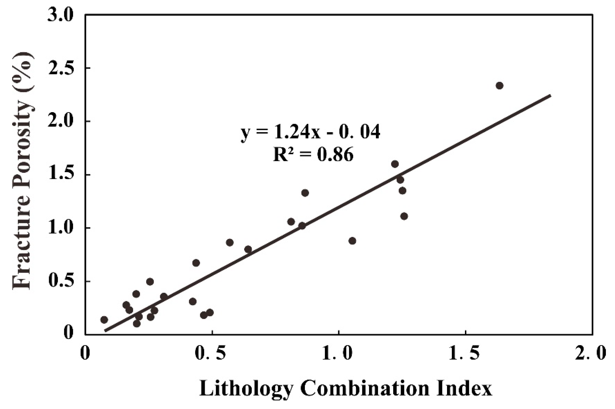
The LCI and fracture porosity present a good linear relationship. The fracture range of the Da’anzhai member extends from 0 to 5%. Thus, the LCI ranges from 0 to 4, according to the corresponding relationship. When simulating a fracture, the fracture porosity can be calculated as follows:
where z1, z2, and z3 denote the shale content at a certain depth, the number of layers, and the shale content in the window, respectively. The constants 1.24 and −0.04 are the parameters simulated by direct correspondence between the LCI and fracture porosity. Other parameters are identical to those described above.
6.2. Fracture Predictions
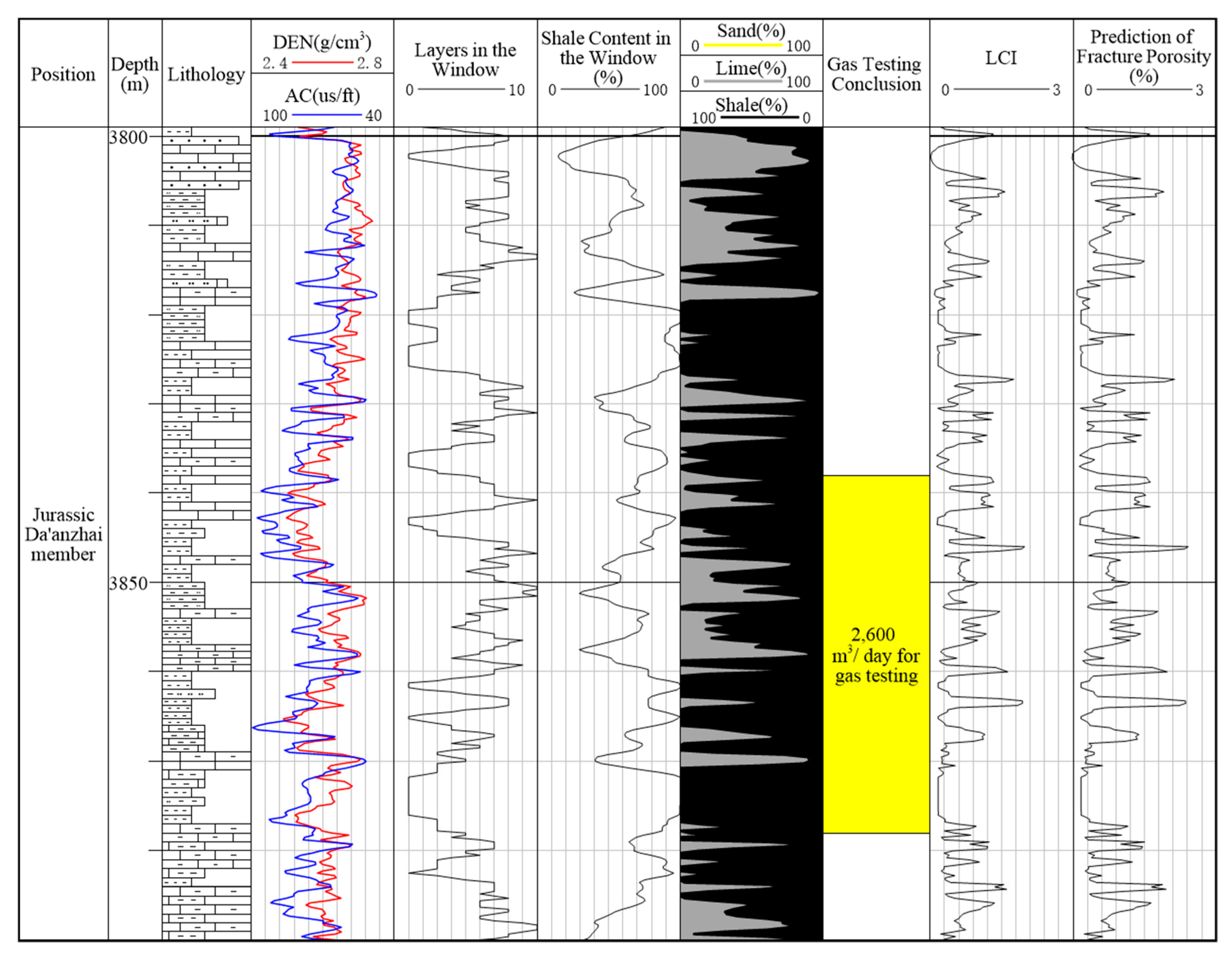
Fracture predictions were made for four wells in Yuanba area, using the methods described in Appendix A (Figure A1, Figure A2, Figure A3 and Figure A4). The prediction results show that the LCI values of the four wells range from 0 to 2.07 after calculation, the simulated fracture porosity ranges from 0 to 2.53%, and the average fracture porosity is 0.63%. The improved results for the gas test and their fracture porosity were higher than the results based on other combinations. There is an elevated development of fractures, due to the lithology combinations of thick-bedded sandstone, sand-shale stone, and thick-bedded shale.
7. Discussions
This method can be used for other areas, and even the formation of other lithologies, such as carbonate rocks or tight sandstone formations. The process, however, must be altered such that the simulated parameters are applicable to the exploration area. Initially, the factors affecting fracture development should be identified and quantified. Lithologies, lithology combinations, tectonic stress fields, total organic carbon, and other factors can all be used as factors that affect fracture development. Nevertheless, these factors must be simplified, as well as the elimination of secondary factors to reserve major factors. Prior to machine learning, we must analyze the influence that single factors have on cracks to obtain different relationships. The corresponding relationship transformation is then made to unify the relationships. If necessary, the choice of the lithology window should also be simulated again, according to the fitting reliability, to obtain the proper window. For machine learning, we must select an appropriate machine learning method that can be verified after adjusting the parameters. The method should also be supported by common mathematical and geological theories. Any abnormal data should be removed during verification. The average value should be taken as the final result after several rounds of verification. The constants in the LCI formula were acquired based on the various function parameters via a single-factor analysis. The corresponding factors that affect the weight of each factor, as well as several unknown numbers, were obtained according to the definitive influencing factors. Finally, the relationship after adjustment was modified into the original relationship, in which the fracture porosity is the dependent variable. This relationship should then be tested and compared with measured data. This study employs the comparison data associated with gas tests, where data such as measured fracture data can also be used to fit other wells that have not been analyzed by the model. The fracture porosity of the new area can be fitted by inputting the variable values of the newly fitted area. Horizontal and vertical fracture development of the entire formation and the entire study area can be computed using this method. Therefore, the fracture development of the whole area can be visually presented by data, which provides a new angle of evaluation for oil and gas exploration.
8. Conclusions
- (1)
- From a lithology combination perspective and the machine learning concept, we established a quantitative characterization model for the LCI and fracture development. The LCI quantifies the complex comprehensive influence that multiple factors have on fracture development, using several formulae to fit the composite function relationship with the fractures and some factors, which yields a quantitative characterization of the fractures. We established the quantitative characterization model of LCI and fracture development by defining this index, such that we can quantitatively predict fracture development.
- (2)
- After determining the LCI formula for a specific area, inputting the values of the various factors that affect the fractures in this area can simulate fracture development in the entire stratum. This method has been used to predict fractures in the Da’anzhai member of the Yuanba area, whose results show that the method is reliable. This method is also applicable in other regions, but the regional parameters must be adapted according to the actual conditions of the region.
Supplementary Materials
Zhengchen Zhang developed the program in the “Adjust” and “choose” section that is available on https://github.com/zhzhch88/Zhengchen-Zhang/tree/LCI free of charge. The instructions are shown in the web link.
Author Contributions
Data collection, data analysis and paper writing, Z.Z.; preliminary idea and technical guidance, P.L.; discussion and proofreading, Y.Y. and K.L.; data provided, J.H.; project supervision, H.Z. All authors have read and agreed to the published version of the manuscript.
Funding
This study was supported by National Science and Technology Major Project (2017ZX05036-004-004) and (2017ZX05005-003-003).
Acknowledgments
Z.Z. would like to thank Sinopec Exploration Company for the providing the project and financial support.
Conflicts of Interest
The authors declare no conflict of interest regarding this manuscript.
Appendix A
Figure A1.
The prediction of fracture in Yuanba 101 well.

Figure A2.
The prediction of fracture in Yuanlu 31 well.

Figure A3.
The prediction of fracture in Yuanba 11 well.
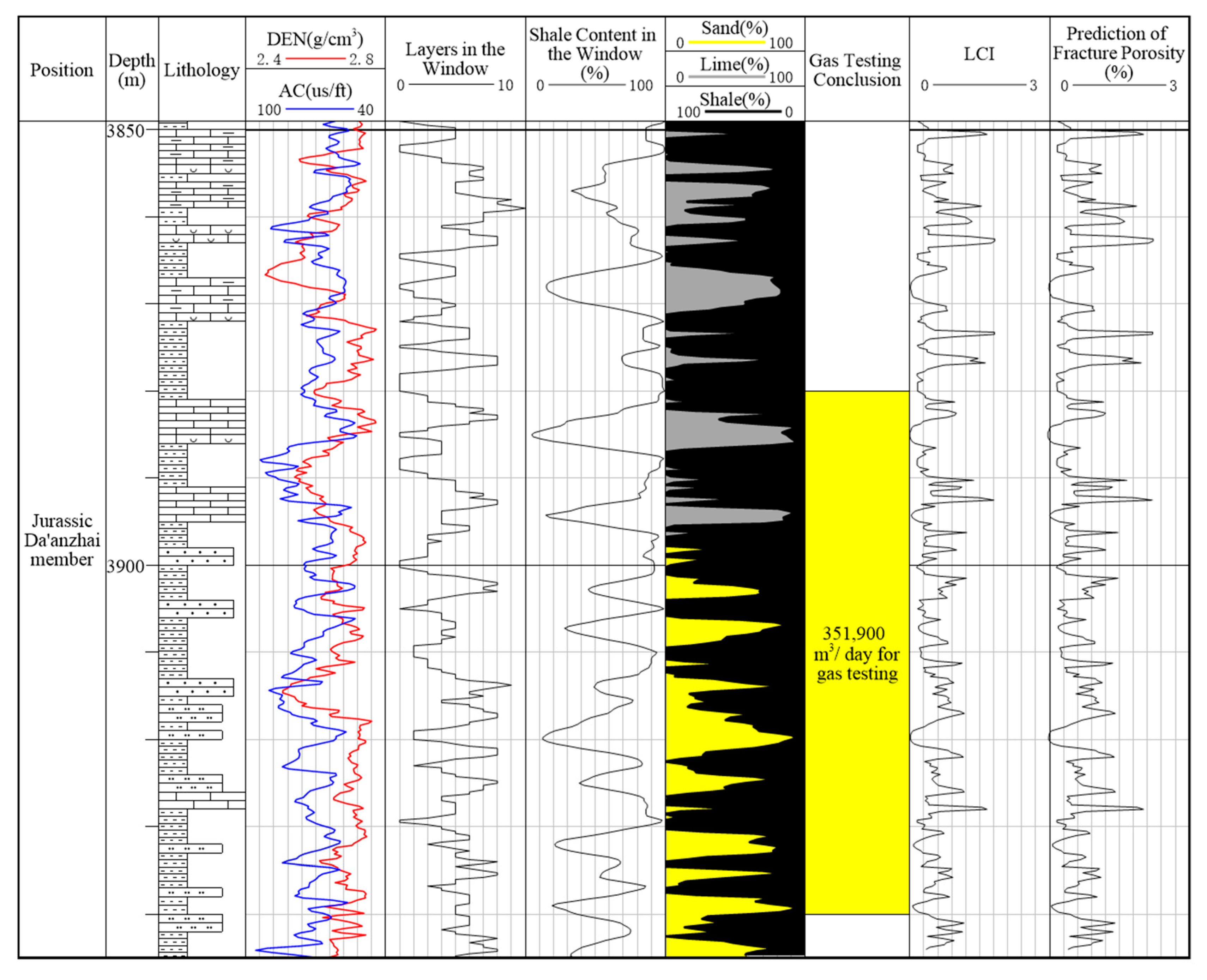
Figure A4.
The prediction of fracture in Yuanba 9 well.
References
- Engelder, T. Loading paths to joint propagation during a tectonic cycle: An example from the Appalachian Plateau, U.S.A. J. Struct. Geol. 1985, 7, 459–476. [Google Scholar] [CrossRef]
- Gale, J.F.W.; Laubach, S.E.; Olson, J.E. Natural fractures in shale: A review and new observations. Aapg Bull. 2014, 98, 2165–2216. [Google Scholar] [CrossRef]
- Gale, J.F.W.; Elliott, S.J.; Li, J.Z. Natural fracture characterization in the Wolfcamp Formation at the Hydraulic Fracture Test Site (HFTS), Midland basin, Texas. In Proceedings of the Unconventional Resources Technology Conference, Denver, CO, USA, 22–24 July 2019. [Google Scholar] [CrossRef]
- Laubach, S.E.; Lander, R.H.; Criscenti, L.J. The role of chemistry in fracture pattern development and opportunities to advance interpretations of geological materials. Rev. Geophys. 2019, 57, 1065–1111. [Google Scholar] [CrossRef] [Green Version]
- Huang, Q.; Angelier, J. Fracture spacing and its relation to bed thickness. Geol. Mag. 1989, 126, 355. [Google Scholar] [CrossRef]
- Ellis, M.A.; Laubach, S.E.; Eichhubl, P. Fracture development and diagenesis of Torridon Group Applecross Formation, near an Teallach, NW Scotland: Millennia of brittle deformation resilience? J. Geol. Soc. Lond. 2012, 169, 297–310. [Google Scholar] [CrossRef]
- Zeng, L.; Li, X. Fractures in sandstone reservoirs with ultra-low permeability: A case study of the Upper Triassic Yanchang Formation in the Odos Basin, China. Aapg. Bull. 2009, 93, 461–477. [Google Scholar] [CrossRef]
- Gale, J.F.W.; Lander, R.H.; Reed, R.M. Modeling fracture porosity evolution in dolostone. J. Struct. Geol. 2010, 32, 1201–1211. [Google Scholar] [CrossRef]
- Rickman, R.; Mullen, M.J.; Petre, J.E. A Practical Use of Shale Petrophysics for Stimulation Design Optimization: All Shale Plays Are Not Clones of the Barnett Shale. In Proceedings of the SPE Annual Technical Conference and Exhibition, Denver, CO, USA, 21–24 September 2008. [Google Scholar] [CrossRef] [Green Version]
- Wang, R.; Hu, Z.; Liu, J. Comparative analysis of characteristics and controlling factors of fractures in marine and continental shales: A case study of the Lower Cambrian in Cenggong area, northern Guizhou Province. Oil Gas. Geol. 2018. (In Chinese) [Google Scholar] [CrossRef]
- Wang, X.; Zhao, M.; Xiang, B. Carboniferous source rocks in the Ludong-Wucaiwan area, Junggar Basin, NW China. Pet. Explor. Dev. 2010, 37, 523–530. [Google Scholar] [CrossRef]
- Zhu, G.; Gu, L.; Su, J. Sedimentary association of alternated mudstones and tight sandstones in China’s oil and gas bearing basins and its natural gas accumulation. J. Asian Earth Sci. 2012, 50. [Google Scholar] [CrossRef]
- Yurewicz, D.A.; Bohacs, K.M.; Kendall, J. 2005. Controls on gas and water distribution, Mesaverde basin-centered gas play, Piceance basin, Colorado. Search Discov. 2005, 105–136. [Google Scholar] [CrossRef]
- Alpaydin, E. Introduction to Machine Learning; MIT Press: Cambridge, MA, USA, 2004. [Google Scholar] [CrossRef]
- Mayer-Schonberger, V.; Cukier, K. Big Data: A Revolution That Will Transform How We Live, Work, and Think; Houghton Mifflin Harcourt Publishing Company: New York, NY, USA, 2013. [Google Scholar] [CrossRef]
- Mulder, E.F.J.D.; Cheng, Q.; Agterberg, F. New and game-changing developments in geochemical exploration. Episodes 2016, 39, 70–71. [Google Scholar] [CrossRef] [Green Version]
- Ross, Z.E.; Men-Andrin, M.; Egill, H. 2018. P-wave arrival picking and first-motion polarity determination with deep learning. J. Geophys. Res. Solid Earth 2018. [Google Scholar] [CrossRef]
- Ouenes, A.; Richardson, S.; Weiss, W.W. Fractured Reservoir Characterization and Performance Forecasting Using Geomechanics and Artificial Intelligence. In Proceedings of the SPE Annual Technical Conference and Exhibition, Dallas, TX, USA, 22–25 October 1995. [Google Scholar] [CrossRef]
- Ouenes, A. Practical application of fuzzy logic and neural networks to fractured reservoir characterization. Comput. Geosci. 2000, 26, 953–962. [Google Scholar] [CrossRef]
- Barman, I.; Ouenes, A.; Wang, M. Fractured Reservoir Characterization Using Streamline-Based Inverse Modeling and Artificial Intelligence Tools. In Proceedings of the SPE Annual Technical Conference and Exhibition, Dallas, TX, USA, 1–4 October 2000. [Google Scholar] [CrossRef]
- Ozkaya, S.I. Using Probabilistic Decision Trees to Detect Fracture Corridors from Dynamic Data in Mature Oil Fields. Spe Reserv. Eval. Eng. 2008. [Google Scholar] [CrossRef]
- Lu, B. Shale Gas. Reservoir Evaluation of Da’anzhai Member in Ziliujing Formation of Lower Jurassic in Eastern Sichuan Basin; Chengdu University of Technology: Chengdu, China, 2015. (In Chinese) [Google Scholar]
- Wang, Y.; Tong, M.; Sun, Y. Reservoir characteristics of Da’anzhai shell limestone tight oil in Sichuan Basin. Acta Pet. Sin. 2019, 40, 42–55. (In Chinese) [Google Scholar]
- Zhou, X.; Liang, B. Characteristics and recognition of Lower Jurassic shell limestone in Yuanba Area of Sichuan Basin. J. Xi Pet. Univ. 2017, 32, 35–43. (In Chinese) [Google Scholar]
- Yan, X. The Sedimentary Facies Study of Lower Jurassic Da’anzhai Member in Fuling Area, Eastern Sichuan Basin; Chengdu University of Technology: Chengdu, China, 2015. (In Chinese) [Google Scholar]
- Zhou, G.; Xu, S.; Ran, X. Pore structure characteristics and control factors of shale in the Da’anzhai formation centrale of Sichuan Basin. J. Northwest. Univ. 2018, 48, 718–728. (In Chinese) [Google Scholar]
- Curtis, J.B. Fractured shale-gas systems. Aapg Bull. 2002, 86, 1921–1938. [Google Scholar] [CrossRef]
- Curtis, M.E.; Sondergeld, C.H.; Ambrose, R.J. Microstructural investigation of gas shales in two and three dimensions using nanometerscale resolution imaging. Aapg Bull. 2012, 96, 665–677. [Google Scholar] [CrossRef]
- Sun, W.; Li, W.; Dong, Z. A new approach to the characterization of shale pore structure. Lithol. Reserv. 2017, 29, 125–130. [Google Scholar] [CrossRef]
- Yuan, Y.; Rezaee, R.; Al-Khdheeawi, A.E. Impact of Composition on Pore Structure Properties in Shale: Implications for Micro-/Mesopore Volume and Surface Area Prediction. Energy Fuels 2019, 33, 9619–9628. [Google Scholar] [CrossRef]
- Yuan, Y.; Rezaee, R. Comparative Porosity and Pore Structure Assessment in Shales: Measurement Techniques, Influencing Factors and Implications for Reservoir Characterization. Energies 2019, 12, 2094. [Google Scholar] [CrossRef] [Green Version]
- Zheng, R.; He, L.; Liang, X. Formation condition of shale gas (oil) in the Lower Jurassic Da’anzhai member in the eastern Sichuan Basin. Nat. Gas. Ind. 2013, 33, 30–40. (In Chinese) [Google Scholar]
- Martin, J. A Geomechanical Approach to Evaluate Brittleness Using Well Logs: Mississippian Limestone, Northern Oklahoma. Master’s Thesis, The University of Texas at Arlington, Arlington, TX, USA, 2015. [Google Scholar]
- Zhao, L.; Wei, W.; Li, Y. The Application of the Multi-Mineral Model in a Block of Southern China. In Proceedings of the 75th EAGE Conference & Exhibition Incorporating SPE EUROPEC, London, UK, 13 June 2013. [Google Scholar] [CrossRef]
- Feng, R.; Wu, Y.; Tao, S. Sedimentary microfacies characteristics and their control on reservoirs in Da’anzhai Member, Lower Jurassic, Sichuan Basin. Pet. Geol. Exp. 2015, 37, 320–327. (In Chinese) [Google Scholar]
- Tan, M. Features and Model of Mixed Siliciclastic-Carbonate Sediments of Da’anzhai Member in Lower Jurassic Ziliujing Formation, Huilong Area, Sichuan Basin; Chengdu University of Technology: Chengdu, China, 2017. (In Chinese) [Google Scholar]
- Yuan, Y.; Rezaee, R.; Verrall, M. Pore characterization and clay bound water assessment in shale with a combination of NMR and low-pressure nitrogen gas adsorption. Int. J. Coal Geol. 2018, S0166516218302702. [Google Scholar] [CrossRef]
- Yuan, Y.; Rezaee, R. Fractal analysis of the pore structure for clay bound water and potential gas storage in shales based on NMR and N2 gas adsorption. J. Pet. Sci. Eng. 2019. [Google Scholar] [CrossRef]
- Loucks, R.G.; Reed, R.M.; Ruppel, S.C. Spectrum of pore types and networks in mudrocks and a descriptive classification for matrix-related mudrock pores. AAPG Bull. 2012, 96, 1071–1098. [Google Scholar] [CrossRef] [Green Version]
- Vapnik, V.N.; Drucker, H.; Burges, J.C. Support. Vector Regression Machines. Advances in Neural Information Processing Systems 9; MIT Press: Cambridge, MA, USA, 1996; pp. 155–161. [Google Scholar] [CrossRef]
- Cherkassky, V.; Mulier, F. Statistical Learning Theory. Learning from Data: Concepts, Theory, and Methods, 2nd ed.; John Wiley & Sons: Hoboken, NJ, USA, 2006; Volume 41, p. 3185. [Google Scholar] [CrossRef] [Green Version]
- Hsieh, W.W. Machine Learning Methods in the Environmental Sciences: Neural Networks and Kernels; Cambridge University Press: Cambridge, UK, 2009; pp. 157–169. [Google Scholar] [CrossRef] [Green Version]
- Li, S.; Yang, F. Classification of Gas-Rich Lithofacies in Continental Shale Formation Based on bi-Langmuir Model and SVM Methods. In Proceedings of the Society of Exploration Geophysicists SEG Technical Program Expanded Abstracts, Dallas, TX, USA, 16–21 October 2016; pp. 3518–3522. [Google Scholar] [CrossRef]
- Aryafar, A.; Moeini, H. Application of continuous restricted Boltzmann machine to detect multivariate anomalies from stream sediment geochemical data, Korit, East of Iran. J. Min. Environ. 2017, 8, 673–682. [Google Scholar] [CrossRef]
- Carranza, E.J.M.; Laborte, A.G. Random forest predictive modeling of mineral prospectivity with small number of prospects and data with missing values in Abra (Philippines). Comput. Geosci. 2015, 74, 60–70. [Google Scholar] [CrossRef]
- Tan, M.; Song, X.; Yang, X. Support-vector-regression machine technology for total organic carbon content prediction from wireline logs in organic shale: A comparative study. J. Nat. Gas. Sci. Eng. 2015, 26, 792–802. [Google Scholar] [CrossRef]
- Shi, G. Superiorities of Support Vector Machine in Fracture Prediction and Gassiness Evaluation. Pet. Explor. Dev. 2008, 35, 588–594. [Google Scholar] [CrossRef]
Figure 1.
The same rock content leads to different lithology combinations: (a) single type, (b) multi-layer type, and (c) cross-bed type.
Figure 1.
The same rock content leads to different lithology combinations: (a) single type, (b) multi-layer type, and (c) cross-bed type.
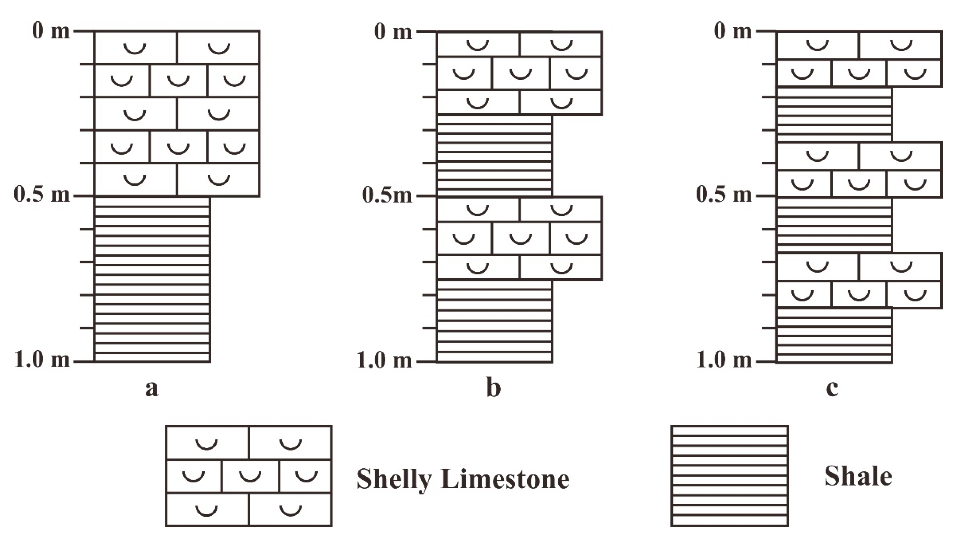
Figure 2.
Fractures (red areas) in mosaic images. (a) Yuanlu 4 well, 3747.18 m, (b) Yuanlu 176 well, 4141.85 m, and (c) Yuanba 122 well, 3560.35 m.
Figure 2.
Fractures (red areas) in mosaic images. (a) Yuanlu 4 well, 3747.18 m, (b) Yuanlu 176 well, 4141.85 m, and (c) Yuanba 122 well, 3560.35 m.

Figure 3.
The relationship between fracture porosity and shale content.

Figure 4.
The relationship between fracture porosity and lime content.
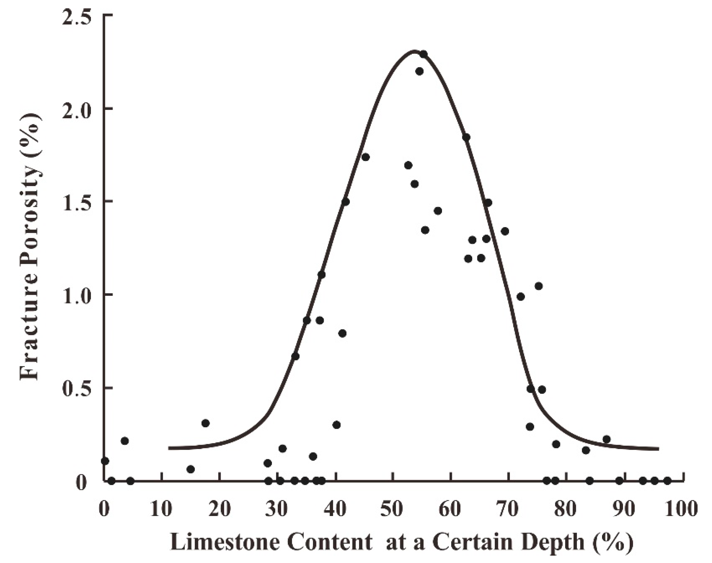
Figure 5.
The results of verification for different levels of windows: (a) 1 m, (b) 2 m, (c) 4 m, and (d) 6 m.
Figure 5.
The results of verification for different levels of windows: (a) 1 m, (b) 2 m, (c) 4 m, and (d) 6 m.

Figure 6.
The relationship between each content and fracture porosity in a window of 2 m.: (a) The relationship between fracture porosity and shale content, (b) The relationship between fracture porosity and lime content.
Figure 6.
The relationship between each content and fracture porosity in a window of 2 m.: (a) The relationship between fracture porosity and shale content, (b) The relationship between fracture porosity and lime content.
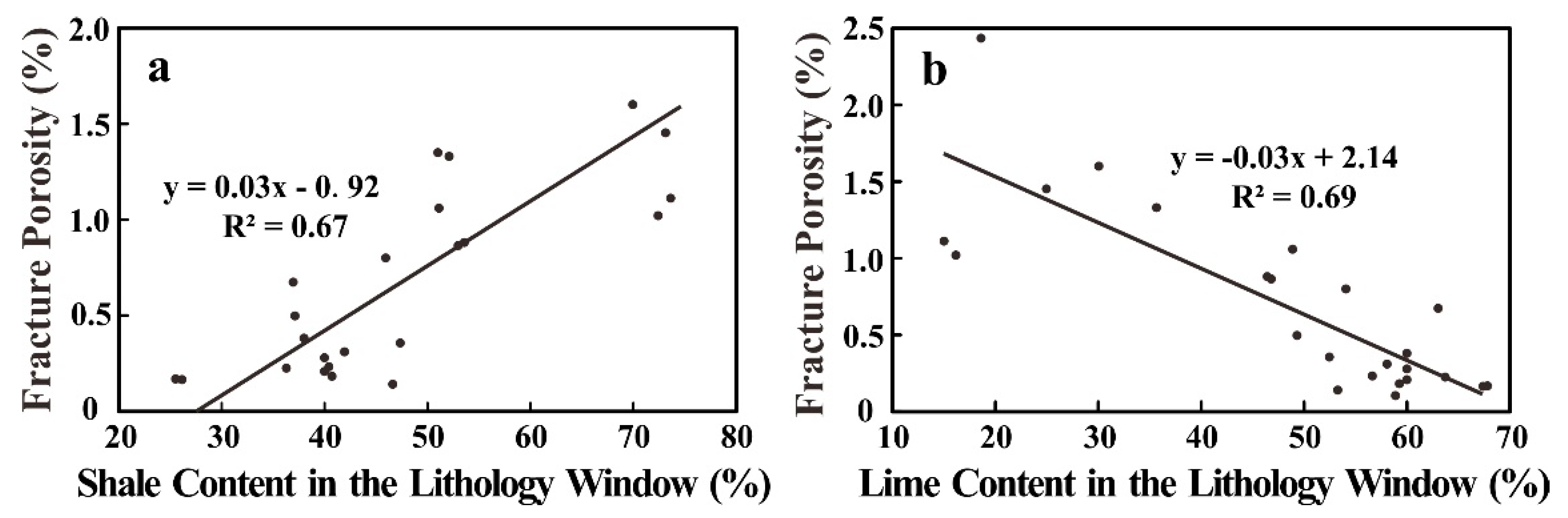
Figure 7.
The comparison of the results obtained from learning repetitions with the test set. Five figures represent five verifications (green represents the true value, and red represents the conjectured value).
Figure 7.
The comparison of the results obtained from learning repetitions with the test set. Five figures represent five verifications (green represents the true value, and red represents the conjectured value).
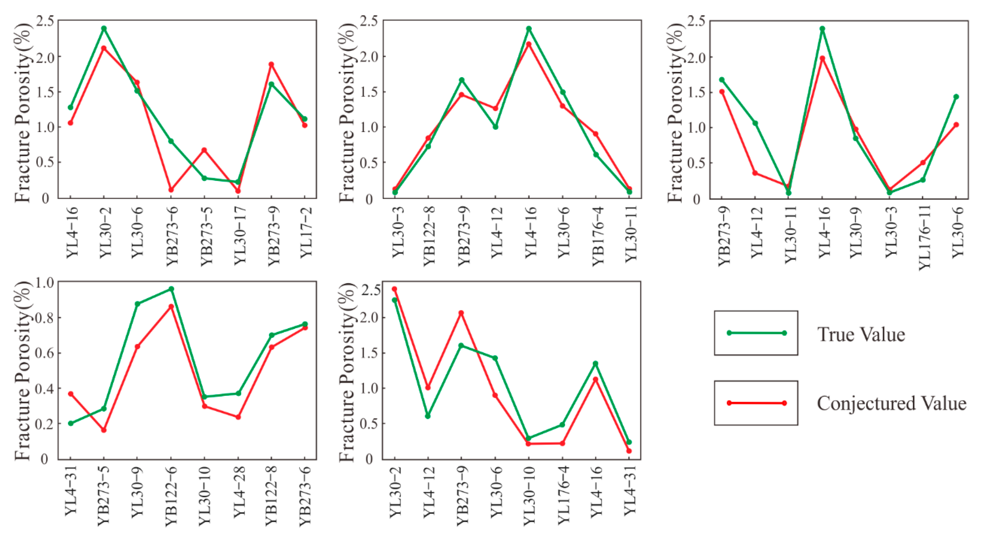
Figure 8.
The relationship between lithology combination index (LCI) and fracture porosity.

Table 1.
The weight of each factor obtained by five machine learning methods and the reliability of each method.
Table 1.
The weight of each factor obtained by five machine learning methods and the reliability of each method.
| Model | Shale Content at a Certain Depth | The Number of Layers | Shale Content in the Window | Reliability |
|---|---|---|---|---|
| Multi-linear regression | 0.19 | 1.12 | 1.53 | 0.48 |
| Decision-making tree | 0.02 | 0.01 | 0.96 | 0.46 |
| Support vector machine | 0.21 | 0.48 | 1.27 | 0.71 |
| K-nearest neighbor prediction | / | / | / | 0.39 |
| Random forest algorithm | 1.94 | 0.33 | 0.46 | 0.39 |
/: no data.
Table 2.
Simulation results and reliability of the support vector machine (SVM) model after parameter adjustment.
Table 2.
Simulation results and reliability of the support vector machine (SVM) model after parameter adjustment.
| Number | Shale Content at a Certain Depth | The Number of Layers | Shale Content in the Window | Reliability |
|---|---|---|---|---|
| The first time | 0.13 | 0.78 | 1.64 | 0.76 |
| The second time | 0.09 | 0.81 | 1.73 | 0.93 |
| The third time | 0.06 | 1.07 | 1.55 | 0.84 |
| The fourth time | 0.12 | 0.70 | 1.52 | 0.76 |
| The fifth time | 0.14 | 0.97 | 1.62 | 0.86 |
| Average value | 0.11 | 0.87 | 1.61 | 0.83 |
© 2020 by the authors. Licensee MDPI, Basel, Switzerland. This article is an open access article distributed under the terms and conditions of the Creative Commons Attribution (CC BY) license (http://creativecommons.org/licenses/by/4.0/).
Share and Cite
MDPI and ACS Style
Zhang, Z.; Li, P.; Yuan, Y.; Liu, K.; Hao, J.; Zou, H. Quantitative Prediction of Fractures in Shale Using the Lithology Combination Index. Minerals 2020, 10, 569. https://doi.org/10.3390/min10060569
AMA Style
Zhang Z, Li P, Yuan Y, Liu K, Hao J, Zou H. Quantitative Prediction of Fractures in Shale Using the Lithology Combination Index. Minerals. 2020; 10(6):569. https://doi.org/10.3390/min10060569
Chicago/Turabian StyleZhang, Zhengchen, Pingping Li, Yujie Yuan, Kouqi Liu, Jingyu Hao, and Huayao Zou. 2020. "Quantitative Prediction of Fractures in Shale Using the Lithology Combination Index" Minerals 10, no. 6: 569. https://doi.org/10.3390/min10060569
Note that from the first issue of 2016, this journal uses article numbers instead of page numbers. See further details here.