Article

Construction and Application of a Knowledge Graph for Gold Deposits in the Jiapigou Gold Metallogenic Belt, Jilin Province, China

1
College of Geoexploration Science and Technology, Jilin University, Changchun 130026, China
2
Geoscience Big Data Analysis and Application Technology Innovation Center, Ministry of Natural Resources, Changchun 130026, China
3
Jilin Branch of China National Geological Exploration Center of Building Materials Industry, Changchun 130033, China
4
College of Earth Sciences, Jilin University, Changchun 130061, China
*
Author to whom correspondence should be addressed.
Minerals 2022, 12(9), 1173; https://doi.org/10.3390/min12091173
Submission received: 23 August 2022 / Revised: 13 September 2022 / Accepted: 13 September 2022 / Published: 17 September 2022

Abstract

:
Over the years, many geological exploration reports and considerable geological data have been accumulated during the prospecting and exploration of the Jiapigou gold metallogenic belt (JGMB). It is very important to fully utilize these geological and mineralogical big data to guide future gold exploration. This work collects the original textual data of different gold deposits in JGMB and constructs a knowledge graph (KG) for deposits based on deep learning (DL) and natural language processing (NLP). Based on the metallogenic geological characteristics of deposits, a visual construction method of a KG for deposits and a calculation of the similarity between deposits are proposed. In this paper, 20 geological entities and 24 relationship categories are considered. By condensing the key KG information, the metallogenic geological conditions and factors controlling the ore in 14 typical deposits in the JGMB are systematically analyzed, and the metallogenic regularity is summarized. By calculating the deposits’ cosine similarities based on the KG, the mineralization types of deposits can be divided into two categories according to the industrial types of ore bodies. The results also show that the KG is a cutting-edge technology that can extract the rich information of ore-forming regularity and prospecting criteria contained in the textual data to help researchers quickly analyze the mineralization information.

Graphical Abstract

1. Introduction

The Jiapigou gold metallogenic belt (JGMB), located in southeastern Huadian, southern Jilin Province, Northeast China, is not only an important gold cluster area in the eastern segment of the northern margin of the North China Craton (NCC), but also the main gold-producing area with proven gold reserves of more than 180 tons [1] in China, in which a dozen gold deposits (Figure 1) and more than 160 gold occurrences have been discovered since 1820. The JGMB has great potential for gold prospecting with the development of gold exploration in the depth of the existing gold deposits, and the new gold deposits have been funded along its southeast extension in recent years. Many studies have been performed on the regional ore-forming geological background, petrology, mineralogy, geochemistry, and genesis of some typical gold deposits and occurrences in the JGMB [1,2,3,4,5]. It can be concluded from previous studies that (1) the gold deposits are of three mineralized types: quartz vein (Banmiaozi deposit, Bajiazi deposit, Jiapigou deposit, and Haigou deposit), altered rock (Songjianghe deposit and Liupiye deposit), and breccia (Toudaoliuhe deposit and Binhugou deposit); (2) the origins of gold deposits belong to the orogenic type [2,6,7,8,9] and the mesothermal one [1,4]; (3) the gold deposits exhibit a multistage gold mineralization processes, with a time span ranging from approximately 230 to 68 Ma; (4) the gold deposits are mainly controlled by the NW-striking Jiapigou fault belt and its related secondary faults; and (5) the gold deposits are closely related to Yanshanian tectono-magmatism [10,11].
These studies further deepen our understanding of the gold mineralization characteristics and gold metallogeny of the JGMB. However, the ages, origin, metallogenic processes, etc. of gold deposits in the JGMB are still debated partly because of the lack of regional comparisons between gold deposits in different spatial locations, of various styles of gold ore mineralization hosted in different country rocks, and with different ore-forming ages. A large number of research papers published in Chinese and English journals, scientific reports on geology and specific reports on ore exploration have been accumulated since the 1960s in JGMB. However, it is difficult to quickly extract some valuable information about ore-forming and ore-prospecting from numerous papers and reports of a dozen or a hundred gold deposits and occurrences with the manual curation method, which is a time-consuming process that requires some experts to read geological papers and reports, and annotate professional terms or sentences that assert some relationship between geological factors. Therefore, how to intelligently read and process from the papers and reports as text files from a dozen or a hundred gold deposits and occurrences and how to quickly extract the necessary information used for investigating the regional gold metallogeny and exploring gold deposits in a gold cluster area are great challenges for geologists and experts in artificial intelligence (AI).
Natural language processing (NLP) and deep learning (DL) are subsets of AI. Automated approaches rely on DL or NLP to rapidly detect terms and sentences of interest containing geological papers and reports. NLP makes it possible for humans to talk with machines, and its goal is to construct systems that can make sense of the written text and automatically perform tasks such as translation, keyword extraction, and topic classification [16]. NLP includes two parts: natural language understanding and natural language generation, which can recognize structured and unstructured textual data.
The concept of a knowledge graph (KG) was proposed by Google in 2012 [17]. NLP and KGs often need to be applied together to give full play to their maximum efficiency. A KG contains entities, concepts, attributes, relations, and other information and can use language understood by both humans and machines to describe the real world in the form of graphs, making the knowledge structure clearer. However, it is single-minded to understand the KG simply as a graph because in the face of massive data, it is usually impossible to display all knowledge structures in the form of a graph on one screen. Therefore, the KG is a semantic network formed by the semantic computing of many texts illustrating knowledge. Its main purpose is to construct a graph according to its relationship with knowledge and search by using the knowledge structure. As AI has developed, KGs have gradually penetrated various fields [18,19,20,21].
Previous scholars have explored the application of NLP and KGs in geological work [22,23,24]. Wang et al. [25] used NLP technology to analyze mineral resources and introduced the workflow of Chinese documents, proving the effectiveness of the designed workflow, and showed the potential of NLP technology in geoscience. Li et al. [26] used the Lala copper mine as an example and studied the method of mining prospecting information in text based on a convolutional neural network (CNN). Holden et al. [27] developed GeoDocA, a geological document analysis system, that can use text mining technology to visually analyze the geological exploration reports. Enkhsaikhan et al. [28] studied the method of understanding ore-forming conditions using the machine reading of text.
The research papers on ore exploration in the JGMB contain a large number of gold deposit-related geological factors and their relations. Identifying these geological factors and relations is of positive significance to rapidly improve the analysis of geological texts. There is a strict corresponding relationship between a deposit and its ore-controlling factors that has the advantage of constructing a KG. However, KG research in the geoscience field is only beginning, and there is a lack of corpora for annotated entities and relations. In this study, the original textual data such as geological exploration reports, published journals and dissertations related to typical deposits in JGMB, are collected. This work carries out research on KGs based on DL and NLP. A visual KG construction method for deposits and a method for calculating the similarities between deposits are proposed. Based on the analysis of texts by AI, rich information about metallogenic regularity, prospecting criteria and deposit genesis can be obtained. Through KG visualization, the relation between geological entities can be displayed. The research shows that this method has important theoretical significance and application value and can rapidly analyze texts and mine potential knowledge.

2. Geological Settings

The JGMB lies between the northern margin of the NCC and the eastern section of the Central Asian Orogenic Belt (CAOB), as shown in Figure 1a,b [12,29,30]. In the study area, the NCC, also known as the Longgang block, is separated from the eastern extension of the CAOB (locally named the Xing’an–Mongolian orogenic belt, a continental margin accretionary belt) by the Jiapigou and Jinyinbie faults with NW strikes, as shown in Figure 1b,c. The strata exposed in the study area are the Neoarchean Jiapigou Group, the Paleoproterozoic Seluohe Group, the early Paleozoic, and the later Paleozoic, Mesozoic, and Cenozoic (Figure 1c). The Neoarchean Jiapigou Group is composed of the Neoarchean Sandaogou Formation, which is exposed in the Longgang block and occurred as inclusions or lenticular bodies in the Neoarchean TTG (trondhjemite, tonalite, and granodiorite) metamorphic complex. The Sandaogou Formation consists of chlorite-hornblende schist, granitic gneiss, chlorite-actinolite, etc., which underwent the metamorphism of low amphibolite to greenschist facies. The Sandaogou Formation hosts most gold deposits in the JGMB such as the Jiapigou deposit and Banmiaozi deposit. The Seluohe Group is distributed in the northern margin of the Longgang block along or around the NW-striking Jinyinbie fault. The Seluohe Group underwent metamorphism of greenschist facies, which is composed mainly of a suite of metavolcanic and metaclastic sedimentary rocks, with rock types of plagioclase amphibolite, amphibole schist, mica chlorite schist, sericite quartz schist, metasandstone, meta-andesite, and tremolite marble.
The LA-ICP-MS zircon U-PB dating data in plagioclase amphibolite range from 2543 to 2527 Ma [31], belonging to the Neoarchean rather than the formerly considered Paleoproterozoic. The Seluohe Group is the ore-hosting strata of the Songjianghe deposit. The early Paleozoic is distributed only in the southwest of the Longgang block and is comprised mainly of detrital sedimentary rocks. The later Paleozoic metavolcanic and metasedimentary rocks are exposed in the Xing’an–Mongolian orogenic belt to the north of the Huifahe fault and Fuerhe fault. Mesozoic volcanic and sedimentary rocks are exposed in the Xing’an–Mongolian orogenic belt to the north of the Huifahe fault or along the Huifahe fault, and the rock assemblage of Mesozoic volcanic rocks is mainly andesite and dacite of the calc-alkaline series. Cenozoic basalts are distributed in the Changbai Mountains and along the faults of Huifahe and Fuerhe. Quaternary deposits are composed mainly of Holocene alluvial and diluvial sediments.
The intrusive activities in the study area can be grouped into five stages: (1) Neoarchean TTG complex, occupying the majority of the Longgang block; (2) Paleozoic diorite and granite intrusions, exposed mainly as batholiths or stocks in the Xing’an–Mongolian orogenic belt to the north of the Fuerhe fault; (3) Triassic monzogranite intrusions, which occurred as stocks in the Xing’an–Mongolian orogenic belt; (4) Jurassic granite intrusions, extensively exposed as batholiths or stocks in the Xing’an–Mongolian orogenic belt, showing a close temporal–spatial relationship with Au mineralization; and (5) Early Cretaceous granite, distributed as only small stocks in the central part of the Longgang block and along the Huifahe fault. Gold deposits in the JMGB are controlled mainly by the NW-striking Jiapigou shear zone and its related faults such as the Jiapigou fault and Jinyinbie fault (Figure 1c) [4,7,32]. All the gold deposits are confined in a zone 40 km long and 4–10 km wide. The gold deposits from the south to the north of the JMGB are Songjianghe, Liupiye, Bajiazi, Jiapigou, Erdaogou, Sidaocha, Sandaocha, Xiaobeigou, Daxiangou, Laoniugou, Caiqiangzi, Banmiaozi, Damiaozi, and Yuanchaogou. The gold deposits in the JMGB can be divided into two types: gold-bearing quartz veins (abovementioned deposits except for the Songjianghe deposit and Liupiye deposit) and disseminated ores (Songjianghe and Liupiye); between them, the former predominates, accounting for approximately 85% of the gold reserve and production [33]. The gold deposits in the JMGB are derived from mesothermal magmatic–hydrothermal processes, with ages ranging from approximately 240 to 150 Ma [31,34].

3. Related Work

The KG can visually show the relationship between geological characteristics. However, at present, research on geoscience KGs is in its infancy. Both the combination of knowledge systems and the construction of large-scale KGs need in-depth study, especially for the following core issues.

3.1. Named Entity Recognition (NER)

NER refers to the entity with specific significance in the text including the name of the deposit, metallogenic geological bodies, metallogenic structure, and metallogenic characteristics. The main task of NER is to detect named entities from the text and classify them into predefined categories. Traditional entity labeling based on statistics considers the frequency or probability of co-occurrences between words and predicts the optimal segmentation sequence through statistical modeling methods such as support vector machine (SVM) [35], hidden Markov model (MHH) [36], and conditional random field (CRF) [37]. With the integration of DL, many new methods have been developed in recent years such as CNNs [38,39], long short-term memory (LSTM) [40], bidirectional long short-term memory (Bi-LSTM) [41,42], recurrent neural networks (RNNs) [43], autoencoders [44,45], and generative adversarial networks (GANs) [46]. Qiu et al. [47] proposed a neural network approach, namely, attention-based bidirectional long short-term memory (Att-Bi-LSTM) with a CRF layer, and used it to extract informational entities describing geoscience information in reports. This method obtained a 91.47% average F1 score in the NER task. Moreover, TensorFlow, PyTorch, and other development environments provide tools for the application of DL.
Labeled data are the basis of supervised learning with neural networks. The quantity and quality of labeled data directly determine the prediction result quality. Geoscience vocabulary has strong professionalism and is greatly different from daily language. At present, there are no systematic labeled geoscience data. However, traditional entity extraction methods must annotate data manually, which results in massive time and labor consumption.
This study used JGMB text data and adopted the NER method based on Bi-LSTM and CRF [28,48]. The Bi-LSTM-CRF model includes three components: the input layer (character embedding), Bi-LSTM layer, and CRF layer, as shown in Figure 2. LSTM is an RNN with a long short-term memory unit. Bi-LSTM is composed of a forward LSTM and a backward LSTM. Both are often used to model contextual information in NLP tasks. Among them, character embeddings are given to a Bi-LSTM. li represents the word i and its left context, and ri represents the word i and its right context. Concatenating these two vectors yields a representation of the word i in its context, ci [49]. To improve the recognition effect of named entities, each character in sentence X is transformed into a vector composed of character embeddings, which are randomly initialized. These character embeddings are the input of the Bi-LSTM-CRF model, and the output is the corresponding prediction label of each character. This work uses the torch.nn.Embedding statement in PyTorch to train the character vectors. The prediction results of the Bi-LSTM layer are input into the CRF layer, which can improve the legitimacy of these predicted labels by adding some constraints. Using this method, a more robust geoscience system based on knowledge extraction can be obtained with low-resource text [50].

3.2. Relation Extraction

As an important task of information extraction, entity relation extraction refers to extracting predefined entity relations from unstructured text based on entity recognition [51]. The relation of entities is made up of triples 〈e1, R, e2〉, where e1 and e2 are entities and R is a relation.
Classic relation extraction methods are divided into four categories: supervised, semi-supervised, weakly supervised, and unsupervised. Supervised relation extraction is divided into feature-based methods and kernel function-based methods. Alokaili et al. [35] and Choi et al. [52] used SVM as a classifier to study the influence of lexical, syntactic, and semantic features on entity semantic relation extraction. In the face of unlabeled data, supervised methods need to manually annotate the training data, which wastes considerable time. Therefore, Huang et al. [53] and Quan et al. [54] then proposed relation extraction methods based on semi-supervised, weakly supervised, and unsupervised methods to solve this problem. Additionally, Brin [55] used the bootstrapping method to extract the relation between named entities; Wang et al. (2018) [24] studied the method of using weakly supervised learning to improve the accuracy of target detection; Hasegawa et al. [56] proposed an unsupervised relation extraction method between named entities. Mintz et al. [57] applied distant supervision in relation extraction.
In traditional relation extraction, the use of NLP leads to error propagation layer-by-layer and affects the effect of relation extraction. Therefore, distant supervised entity-relation extraction methods based on DL including CNN, RNN, LSTM, and other network structures [58,59,60] have become a research focus due to their ability to alleviate the propagation of labels and feature extraction errors. In recent years, scholars have proposed a variety of improvements based on the above basic methods such as the fusion of piecewise convolutional neural networks (PCNNs) and multi-instance learning [61], the COTYPE model [62], and the residual network proposed by Huang and Wang [63], which all enhance the effect of relation extraction.
In 2014, based on the mechanism of human visual attention, Bahdanau et al. applied the attention model to NLP [64,65]. Moreover, attention models have been applied to machine translation based on neural networks and have achieved good results [66]. With the development of DL, attention mechanisms have been widely used due to their excellent performance. Attention-based bidirectional long short-term memory networks (Att-Bi-LSTM) [67] add an attention layer after the Bi-LSTM structure, which can capture the most important semantic information in a sentence.
In this work, Att-Bi-LSTM was used to recognize the entity relation of KGs for gold deposits. Figure 3 shows the neural network architecture of the Att-Bi-LSTM model. This model contains five components: (1) the input layer inputs the sentence to this model, xi represents each word in the sentence, and T represents the number of words in the sentence; (2) the embedding layer maps each word xi in the sentence to a low dimensional vector ei; (3) the LSTM layer, the Bi-LSTM layer inputs the word vectors of the training set obtained from the embedding layer into the forward and backward LSTM, respectively, to obtain high-level features; (4) the attention layer produces a weight vector, and weights the output of each LSTM step to obtain the sentence-level feature vector; and (5) in the output layer, the softmax activation function is used to obtain the final probability of each classification.

3.3. Entity Alignment

After relation extraction, the objective of obtaining the entity and relation information from unstructured data is achieved. However, in geological KGs, it is common for entities to have multiple words and one meaning. For example, the Jiapigou fault can also be named the Dalazi–Jiapigou fault. Therefore, this knowledge needs to be integrated through entity alignment to improve its quality.
Entity alignment can also be called coreference resolution. The goal of entity alignment is to distinguish whether these entities are the same entity by comparing and calculating the similarity between different entities, in order to solve the problem that one entity corresponds to multiple names. The similarity calculation expresses the similarity degree between entities through mathematical calculation. Traditional similarity calculation methods include the Levenshtein distance [68], Jaccard similarity coefficient [69], cosine similarity [70], term frequency-inverse document frequency (TF-IDF) [71,72], and Jaro-Winkler [73]. Volz et al. (2009) [74] provided a number of similarity metrics to calculate the similarity values of strings, URLs, numeric, and dates. In 2014, Vrandecic and Denny et al. [75] defined some feature templates for alignment and achieved good results.
The computation process of the entity alignment algorithm based on the similarity of string and manually defined features is relatively simple. However, because only character-level features are used to measure the similarity of entity categories, the implicit semantic information cannot be captured, resulting in low alignment accuracy. Subsequently, many graph-based entity alignment methods have been proposed. In 2009, Niu X and Rong S et al. [76] studied the measurement index of word sense disambiguation based on the graph method. The similarity of entities based on KGs uses the representation learning algorithm related to the graph structure, which is divided into network representation learning and KG representation learning. Network representation learning includes LINE, node2vec, and DeepWalk [77,78,79]. KG representation learning includes TransE, TranSparse, TransR, and TransH [80,81,82,83]. Using representation learning, entities in KGs can be vectorized. Compared with the similarity calculation based on the textual level, the entity vector obtained by this method can significantly improve the effect.
In recent years, word embedding, as a method of mining the deep-seated related semantics of words, has attracted great attention [84,85,86]. In particular, when using NLP to calculate the text similarity, the text needs to be vectorized first, so the finer-grained text is represented as word embedding. Different word embedding construction methods have different influences on sentence similarity calculation results [87,88]. In the actual application process, it is necessary to choose the appropriate algorithm according to the text situation. Word embedding is based on the core idea [89] that “words with similar context also have similar semantics”. Characters or words are mapped into a vector space, so that words with similar semantics have similar directions in the vector space. Therefore, the alignment method based on word embedding can learn the deep semantic information of words from the corpus to effectively improve the alignment accuracy. Santos et al. [90] calculated the similarity based on the word vector of place names. The results show that this method is superior to the traditional alignment method based on the edit distance.
In this context, this work takes the geological entities of the JMGB as the research object and carries out joint entity alignment method research. This work considers the similarity between entities from two aspects. One is the edit distance similarity of entity names: the entities used in this paper are all geological domain entities, and the entity names are all string types. If the similarity of entity names is high, the probability that these two entities are the same entity is also high. The second is vector similarity: if two entities with similar semantics have a higher similarity of word vectors, then they are also more likely to be the same entity. Based on the above two cases, the weighted sum of the edit distance similarity and the word vector similarity is taken as the final similarity of the two entities. This method can consider the similarity of entities at both the string and semantic levels. The formula is as follows:
s i m ( a i , b i ) = α s i m l e v ( a i , b i ) + ( 1     α ) s i m w o r ( a i , b i )
where ai and bi are two entities to be aligned; α is the weight coefficient; sim(ai,bi) is the similarity of entities to be aligned; simlev(ai,bi) is the edit distance similarity; and simwor(ai,bi) is the word vector similarity. We set the value of α and selected p as the threshold for whether the entity pair was aligned, that is sim(ai,bi) ≥ p, and two entities were considered the same entity.

3.3.1. Edit Distance Similarity

The Levenshtein distance is a kind of edit distance. This algorithm was proposed by Levenshtein [91]. Entity similarity is calculated according to the Levenshtein distance algorithm, which is called the Levenstein ratio, and the formula is as follows:
s i m l e v ( a i , b i ) = 1 Idist l e n g t h ( a i ) + l e n g t h ( b i )
where Idist is the class edit distance, which refers to the minimum number of edits needed to change string ai into string bi. In this case, the insertion or deletion of a string is edited once, and the replacement of a string is edited twice; length(ai) is the length of string ai; and length(bi) is the length of string bi. We used the Levenshtein toolkit in Python and used the levenshtein.ratio statement to compute the similarity of two entities.

3.3.2. Vector Similarity

The word2vec proposed by Mikolov et al. [92] is widely used in comparing the similarity between words. In this paper, word2vec was used to transform the entities to be aligned into word vectors, and then cosine similarity was used to calculate their similarity, which represents the semantic similarity of entities. The cosine similarity formula is as follows:
s i m w o r ( a i , b i ) = i = 1 n a i × b i i = 1 n a i × i = 1 n b i
Formula (3) shows that the range of cosine similarity values is [0, 1], and the greater the value, the higher the similarity. ai and bi represent the word vector set of the geological entities. In this paper, the gensim toolkit in Python was used to train word vectors by Gensim.models. The Word2Vec statement and the cosine similarity between entities were calculated by the cosine_similarity statement. The alignment entities were obtained by setting the threshold.

3.4. Visualization of KGs

Zhou et al. [93] considered that the geoscience KG is a clear display of all knowledge nodes and their relations in the field of earth science. Therefore, it is an important challenge to construct a geoscience KG by integrating the complex characteristics, computational attributes, and knowledge relations and rules from the nature of the graph structure. At present, typical KGs include DBpedia, YAGO, Wikidata, OpenCyc, and Freebase [94,95]. These resources cover knowledge in different fields, and the content is constantly enriched as human knowledge grows. KGs are usually stored in triples: <concepts, relationships, attributes>. Common graph databases mainly include OrientDB, Infinite Graph, Neo4j, and Titan [96]. In addition to being a visualization tool, Protégé [97] is used for constructing ontologies, relationships, attributes, and instances in the semantic web. As a science mapping tool, CiteSpace [98] is designed to facilitate the detection of emerging trends and abrupt changes in the scientific literature.
Among them, Neo4j is very suitable as the storage database of KG because of its good support for graph data, large amount of data storage, and support of multiple retrieval methods. By using Cypher, developers can query relevant data and display them in the control window, and return the results in the JSON, XML, and table formats. KG is widely used in NLP such as for auxiliary decision-making, semantic search, and intelligent question answering [99,100,101]. Neo4j creates the contents of the database through Cypher statements and supports external data import from CSV. In this work, entities, attributes and their relations to each deposit are classified and sorted into CSV files, and they are imported in batches through the LOAD CSV statement, new nodes are added to the database through the MERGE statement, and the relations between nodes are created through the MATCH statement.
Due to the deposit formation complexity, it is difficult to effectively integrate and analyze massive geological and mineralogical big data. There is still a lack of research on the intelligent mining of origin information and the discovery of metallogenic geological regulation from large geological and mineralogical big data. In this study, visualization technology based on KGs was used to explain and analyze geological textual data, and the node-edge structural model was used to associate the origin and evolution of gold deposits. The research was used to establish KGs for deposits based on Neo4j and then discover the overall formation mode of mineral resources. Visualization based on KGs can facilitate researchers in analyzing the spatial distribution of data and enhancing the interpretation ability of large amounts of geological data.

4. Construction of KG for Ore Deposits

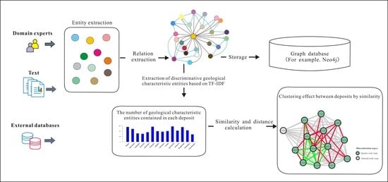
4.1. Basic Ideas and Algorithm Flow

Figure 4 illustrates the framework for KG construction. Through the knowledge acquisition, annotation, and extraction of entities, relations and attributes in the text describing typical gold deposits in the JGMB, a KG for gold deposits with application functions was constructed. The construction process was divided into the following steps. (1) Text on relevant deposits in the JGMB was input, the geological entities of the corresponding deposits were extracted through DL, and an NER dataset of deposits was formed. (2) The relationship network between entities was constructed through relation extraction. (3) The entities were aligned. (4) The entities and relations were stored in Neo4j. The TF-IDF values of these geological entities were extracted based on establishing the KG, and the similarity between different deposits was calculated by cosine similarity.
The core idea of deposit visualization and interpretability based on a KG is to show the relations between deposits through graphs and distinguish the differences between deposits through the similarity of geological characteristics. Based on these design ideas, the proposed method includes three cores: (1) extracting text-based metallogenic information; (2) establishing a KG for the deposit model, and (3) constructing interpretable deposit characteristics. Among them, “constructing interpretable deposit characteristics” aims at the problem that the existing geoscience KG model lacks quantitative interpretation. Based on the geological information extraction of typical deposits in the JGMB, the relations between deposits were constructed, and the similarity between deposits was calculated. Then, quantitative interpretation of the mapping relations between deposits in the metallogenic belt was realized.

4.2. Entity Extraction

Entity extraction is the key input of KG visualization based on DL. At present, there is no mature entity recognition method and no public dataset available for the construction of geoscience KGs. In this work, by collecting the textual data of gold deposits in the JGMB, the corresponding entity extraction was carried out under the guidance of domain experts, and the NER dataset of these deposits was constructed.
Corpus construction. A total of 266 papers and dissertations related to typical gold deposits in JMGB were retrieved and downloaded from the China National Knowledge Infrastructure (CNKI). Among them, 120 were randomly selected for model training and the other 146 were used for model prediction. Since these collected documents were stored in PDF format, the document format needed to be converted to text format data first. The contents of these documents were cleaned, and after removing the drawings and tables, 7014 sentences and 527,449 characters were obtained in the labeled dataset. The unlabeled dataset contained 8802 sentences and 671,489 characters.
Entity category. An entity in the KG refers to the general name of various geological characteristics related to ore deposits. Based on the metallogenic geological body, metallogenic structure, and mineralization characteristics, a total of 20 categories of entities were extracted, as follows in Figure 5.
Basic deposit information was extracted: (1) location such as Dunhua City or Huadian City; and (2) the name of the deposit such as the Songjianghe gold deposit and Liupiye gold deposit.
Metallogenic geological bodies refer to geological bodies that are closely related to the deposits in time, space, and origin and include the following seven entities: (1) group such as the Jiapigou Group and Longgang Group; (2) formation such as the Laoniugou Formation and Xinkaihe Formation; (3) metamorphic rocks such as amphibolite and marble; (4) plutons such as the Huangniling pluton and Wudaoliuhe pluton; (5) intrusive rocks such as granodiorite and adamellite; (6) extrusive rocks such as basalt and rhyolite; and (7) sedimentary rocks such as dolomite and siltstone.
Metallogenic structure refers to the structure that controls the spatial position, shape, scale, occurrence, and internal structure of geological bodies. The metallogenic structure includes the following four entities: (1) geotectonic locations such as the northeastern margin of the NCC and the Xingmeng orogenic belt; (2) regional faults such as the Huifahe fault and Ji’an–Songjiang fault; (3) secondary faults such as the Jiapigou fault and Jinyinbie fault; and (4) fault characteristics such as brittle fault, brittle–ductile fault, and ductile fault.
Mineralization characteristics refer to those that can directly indicate the locations of ore bodies and have special significance for prospecting prediction. The mineralization characteristics include the following seven entities: (1) metallogenic stages such as the milky-quartz stage and quartz-pyrite stage; (2) deposit types such as altered rock-type and quartz vein-type; (3) geological time scales such as Cretaceous and Jurassic; (4) minerals such as pyrite and hematite; (5) dykes such as diorite porphyrite and syenite porphyry; (6) wall rock alterations such as chloritization and pyritization; and (7) ore body shapes such as veins, lenticular veins, and thin veins.
Data annotation. A total of 527,449 characters in 7014 sentences were annotated as a corpus, and the corresponding domain dictionary was generated. After manual annotation and verification, an NER dataset of ore deposits in the JGMB was formed. The annotation rules were set as follows: (1) entity boundary detection, for example, correctly identifying the Seluohe Group rather than Seluohe; and (2) determining the category of the entity, for example, pyrite is a mineral entity rather than a rock entity. In this paper, the BIO annotation method was used. B represents the beginning of an entity, I represents the inside of an entity, and O represents a nonentity. These data are divided into the training dataset, verification dataset, and test dataset at a ratio of 8:1:1, as shown in Table 1.
Experiment. The essence of NER is a sequence labeling problem, that is, classifying each word in the sequence. In this paper, accuracy (ACC), precision (P), recall (R), and F1 [102] were used for the NER evaluation metrics. The configuration of the experimental environment is shown in Table 2. The hyperparametric settings of model training are shown in Table 3.
Evaluation. We selected the Bi-LSTM-CRF model and compared it with the HMM, CRF, and Bi-LSTM models to compare the accuracy of different methods on the geological NER task. As shown in Table 4, the accuracy of HMM was low. CRF was better than Bi-LSTM, but slightly lower than Bi-LSTM-CRF. The experimental results showed that the Bi-LSTM-CRF model had a better entity recognition effect than other models, which can meet the requirements of the construction of the deposit KG.

4.3. Relation Extraction

Discrete nodes are obtained after entity extraction, so it is necessary to determine the relationship between entities to form a network knowledge system. The Att-Bi-LSTM model was used to ensure the accuracy of relation extraction. By default, this method knows the relationship categories contained in all texts. In this case, relation extraction is a problem of text classification. A sentence and two entities contained in the sentence are the inputs, and the category of relation is the output.
Dataset. Currently, there is a lack of public datasets in the field of geology. In this paper, 7014 sentences in the dataset for constructing the NER task in Section 4.2 were used for the relation extraction experiments. The approach taken in this paper was to identify the entities contained in each sentence according to the geological entity dictionary. Through the permutation and combination of entities in sentences, the possible relations are found, and then the relation dataset is constructed. The label categories in the dataset include sentences, entities, and relations. A sentence may contain more than two geological entities. To solve this situation, sentences containing multiple entities are exhaustive until all possible situations are traversed. For example, the sentence “the types of wall rock alteration of the Songjiang gold deposit include pyritization, chloritization, etc.” includes two cases, namely, <Songjiang gold deposit, wall rock alteration, pyritization> and <Songjiang gold deposit, wall rock alteration, chloritization>, which need to be repeated twice. The dataset constructed in this paper contained a total of 80,011 triples, of which 60,000, 10,000, and 10,011 were randomly selected as the training dataset, validation dataset, and test dataset, respectively. Based on the output, relations were defined under the guidance of domain experts. In terms of the definition of the relation type, this paper divided the entity-relation based on the results of DL into two categories: (1) the relationship between ore deposit entities and their geological characteristic entities indicates that geological characteristics play a role in the ore deposits, and the relationship points from the deposit name to the geological characteristic entities such as wall_rock_alteration, metallogenic_stage and secondary_fault; (2) the relationship between the geological characteristic entities such as contains, associated_with and occurs_in. Figure 5 shows the KG for the deposit model based on the algorithm in this paper. Finally, 24 predefined relations and 1 other relation are constructed, as shown in Table 5.
Word embedding. According to the characteristics of the Chinese language, the Jieba toolkit in Python was used to segment sentences to improve the performance of the model. Due to the large number of proper nouns in the geological field, to improve the accuracy of word segmentation, this paper used the trained Bi-LSTM-CRF model to identify the entities in the prediction dataset in the corpus, added these entities to the domain dictionary, and built a dictionary of stopping words to reduce the word segmentation errors.
Word vectors were trained using the continuous bag of words (CBOW) model in word2vec. The CBOW model parameters were set as follows: the sliding window size was 5, the number of training iterations was 5, and the dimensions of the word vector were 50, 100, and 200. Under the supervision of the domain dictionary, all 15,816 sentences in the corpus were segmented and trained to obtain 13,645 word vectors.
Model test. In this paper, the Att-Bi-LSTM model proposed by Zhou et al. (2016) [67], the CNN model proposed by Nguyen et al. (2015) [103], and the RNN model proposed by Zhang et al. (2015) [104] were used for relation extraction. The effect of different word vector dimensions on the training accuracy was verified. The three models used the same hyperparameters, as shown in Table 6. Among them, the heights of the filters used in the CNN were 3, 4, and 5.
Experimental. As seen in Table 7, the ACC, P, R, and F1 scores of the Att-Bi-LSTM model were slightly improved compared with those of the other two models. In contrast, this method could better extract the relationship information between geological entities. Experimental results demonstrated that for the dataset used in this paper, the larger the word vector dimension, the better the training effect. When the word vector dimension was 200, the F1 score of the Att-Bi-LSTM model could reach 91.01%.

4.4. Knowledge Fusion

Data cleaning. AI can maximize the exploration of entities and relations in texts to save labor costs. In this paper, the trained Bi-LSTM-CRF and Att-Bi-LSTM models were used to extract entities and relations from the predicted dataset, respectively. After integrating with the training dataset, the triples for constructing the KG were formed. As shown in Table 8, there are two main problems. First, relatively few relations are effectively annotated. More than 90% of the relations in the dataset were labeled Other, meaning that the relations between entities in these sentences were not predefined. Second, the relation types were not balanced. Common relations have more labeled sentences, while some uncommon relations only have a few labeled sentences.
Therefore, the triples predicted by the model had redundant or even wrong information, and the relations should be further cleaned. At this stage, the following processes were carried out: (1) the same triplets were combined, 15,356 were integrated into 7295 non-repeated triples, and the occurrence times of each triplet were recorded; and (2) according to predefined entity categories and relation categories, we used Neo4j to establish nodes and relations between nodes, and exported them using the Export CSV statement. The version of the Neo4j Community Edition used in this work was 4.2.5. This step can remove these incorrect triples. For example, the semantic relation of triples <Jiapigou gold deposit, dyke, rhyolite> was not in the predefined semantic relationship. After this step, 5168 valid triples remain after cleaning.
Entity alignment. After data cleaning, entities from different sources need to be aligned to ensure the reliability of the KG. The entity alignment method used in this paper included five components. (1) In the face of a large number of entities in the corpus, if all entities are considered as candidate entities and the similarity is compared one by one, the efficiency of the entity alignment will be affected. To improve efficiency, this paper classified entities according to their categories and aligned entities of the same category to establish a candidate set. (2) Word vectors that can express the semantic information of geological entities are generated according to the corpus. The experiments in Section 4.3 have proven that when the dimension of the word vector is set to 200, it can express more semantic information. Therefore, the dimension of the word vector used for entity alignment was also set to 200. (3) According to the generated word vector, the semantic similarity of different entities was calculated. (4) According to the edit distance of the entity name, the similarity of different entities is calculated. (5) The joint entity alignment results were calculated and evaluated according to vector similarity and edit distance similarity.
Comparison of model architectures. Since there were no labeled data, to verify the effectiveness of the proposed entity alignment method, we annotated the entity alignment candidate set. If two entities pointed to one entity, we labelled it as 1. Otherwise, it was labeled 0, and a total of 28,824 annotated data were obtained. The entity alignment methods based on edit distance and word vector proposed in this paper were all unsupervised algorithms. We conducted experiments and compared the effects of these methods on the same set.
The experimental results of the ACC, P, R, and F1 scores of each entity alignment method are shown in Table 9. Table 9 shows that the joint entity alignment method used in this paper achieved the best effect by setting the threshold as 0.67. The experimental results showed that the algorithm worked best when α was set to 0.1, as shown in Figure 6. The method can also be ranked according to the similarity score, which is convenient for experts to further screen, save time, and improve accuracy. The principle of entity alignment used in this work is that if A is aligned with B and B is aligned with C, then the A and C entities can be considered as aligned regardless of whether the similarity score between A and C exceeds the threshold. Finally, the knowledge base of the KG was verified manually, and then the KG was constructed by Neo4j. There were 350 nodes and 2181 edges in the KG.

4.5. The Application of the KG

Due to the spatiotemporal nature of geoscience data, almost all entities can be visually displayed on the KG. Therefore, constructing the expression form of the KG for deposits based on the “entity-relation” can be used to indicate the complex coupling relationship between the geological characteristics related to gold deposits in the metallogenic belt. As shown in Figure 5, A1 and A2 are two nodes representing the fault structure, and the edge between them represents the comparative relationship between a secondary fault and the fault characteristics in a specific state. The fault characteristics of the secondary fault are constantly changing over time; for example, the Jiapigou fault may have three different fracture properties: brittle fault, ductile fault, and brittle–ductile fault. Therefore, there is a complex correlation between seemingly independent geological entities.
Extracting key geological entities. In the JGMB, two deposits with the same origin usually have highly similar geological characteristics. Two deposits of different origins may have different geological characteristics. These differences between deposits can be distinguished by KGs. In this paper, the idea of TF-IDF was analogized, and a key geological entity extraction method based on KGs for deposits was proposed.
TF-IDF is a statistical method [105]. TF-IDF is often used to assess how important a word is to a document. The more important the word, the more likely it is to be the keyword of the document. TF-IDF is often used in keyword extraction. In this work, the concept of TF-IDF was introduced into the importance identification of geological entities, where TF refers to the frequency of a geological entity appearing in all deposits, and IDF indicates the general importance of a geological entity to all deposits in the dataset.
By multiplying TF and IDF, the TF-IDF of all geological entities of each deposit can be obtained. The higher the importance that a geological entity is to the deposit, the greater its TF-IDF value, and the better discriminant ability of the entity for a given deposit. The formula is as follows:
T F × I D F ( i , j ) = T F i j × I D F i = n i j k n k j × log ( | D | 1 + | D i | )
where n i j is the number of occurrences of geological entity i in deposit j, and k n k j is the total number of occurrences of all geological entities in deposit j. | D | is the total number of deposits, and | D i | is the number of deposits containing geological entity i. This method identifies the importance of each geological entity to all deposits and specific deposits by calculating the frequency of the occurrence of each geological entity in the KG. The entity of geological characteristics is the text type. Textual entities can represent the characteristics as a collection of characteristic words and then count their TF-IDF values.
Similarity and distance between deposits based on cosine similarity. An important problem in the KG for deposits is, given two deposits, how to assess whether they are similar and their degree of similarity. This paper introduces the idea of cosine similarity and proposes a calculation method of cosine similarity between deposits based on the TF-IDF value of geological entities. This similarity representation is close to the method of human understanding, and it is easy to add other external human knowledge with strong scalability. The core idea is to use the same geological entities and their TF-IDF values of different deposits in the KG to represent the similarity between deposits. Theoretically, the greater the same geological entities between the two deposits and the greater the TF-IDF value of the geological entities, the higher the similarity between the two deposits.
The steps to calculate the cosine similarity of ore deposits are as follows: (1) the geological entities of each ore deposit are counted; (2) geological entities are mapped into TF-IDF vectors; and (3) the similarity of ore deposits is compared pairwise by a nested loop. In this work, the sklearn toolkit in Python was used to calculate TF-IDF and cosine similarity, which were completed by the TfidfVectorizer statement and cosine_similarity statement, respectively.
Figure 7 illustrates the method by taking some geological entities of deposit A and deposit B as examples. The nodes in Figure 7 represent the two deposits and their geological entities, and the values on the edge represent the TF-IDF values of deposits with different geological entities. The similarity between deposit A and deposit B depends on the number of common geological entities and their TF-IDF values. After calculation, the cosine similarity between these two deposits was approximately 0.47. Gephi software [106] was used to visualize the distance of the similarity matrix. The greater the similarity, the closer the distance between deposits. The visualization of clustering results among typical gold deposits in the JGMB can be obtained.

5. Application of the KG in the JGMB

5.1. Visualization of the KG

Regional magmatic rocks and dykes. There is a strong magmatic activity in the JGMB, and magmatic rocks of different ages and types are exposed including Archean TTG and phanerozoic granites and dykes. The exposed rocks in the study area include mainly granodiorite, granite, syenite, monzonite, granite porphyry, diabase, lamprophyre, and many Au-bearing quartz veins. Figure 8 clearly shows the relationship between the deposits and magmatic rocks in the study area. In terms of relationships, dykes are closely related to gold deposits and are an important magmatic rock condition for gold mineralization, as shown in Figure 9. These results show that magmatic evolution is closely related to regional tectonism and mineralization [2,3,107].
Regional metamorphic rocks, extrusive rocks, sedimentary rocks. The metamorphic rocks exposed in the study area mainly include mylonite, gneiss, schist, slate, and granulite; the extrusive rocks mainly include andesite, basalt, and rhyolite; and the sedimentary rocks mainly include limestone, mudstone, and glutenite. The relationship between gold deposits and the outcropping rocks of each stratum is shown in Figure 10.
Regional structures. The regional structure of the JGMB includes folds and faults, as shown in Figure 11. Among them, the fold structures are the Banmiaozi anticline, Hongqiling syncline, Bajiazi anticline, etc. The regional faults include the Huifahe and Ji’an-Songjiang faults. Among them, the Huifahe fault activity is the most intense. The distribution direction of Mesozoic and Cenozoic faulted basins, sedimentary formations, and late Yanshanian granites in the area are controlled by this fault [2].
Three parallel faults are successively distributed from NE to SW: the Fuerhe, Jinyinbie, and Jiapigou faults; these faults are part of the secondary Huifahe fault. Among them, the Jiapigou fault controls the spatial distribution of deposits in this metallogenic belt.
The analysis of metallogenic-tectonic settings is an important way to distinguish the types of deposits. As shown in Figure 1c and Figure 11, from the ore-controlling structural conditions, each deposit in the western section of the JGMB is adjacent to the Huifahe fault. The Songjiang gold deposit, located in the eastern section of the JGMB, is controlled by the Jinyinbie fault and has the characteristics of ductile activity. The gold deposits in the metallogenic belt are generally superimposed on brittle–ductile deformation and brittle deformation based on early ductile deformation, and the ore bodies are located mainly in the late superimposed brittle fault system.

5.2. Extraction of Key Geological Characteristic Entities

For two similar deposits, the coincidence rate of geological entities may be very high. Therefore, this paper explored whether the characteristics of different deposits could be accurately distinguished by geological entities and their relations. This section uses all of the entities in the KG to calculate the TF-IDF values of the geological entities of each deposit. Table 10 lists the geological entities of the top 10 TF-IDF values of each deposit and arranges them from high to low according to the TF-IDF values.
Although the valuable information contained in the text is often related to high-frequency content words [108], some low-frequency words are also important [109]. TF-IDF is a method to extract low-frequency words that contain important information, and to evaluate the importance of a word to a document. In other words, when a geological entity occurs many times in one deposit, but rarely in others, it has some discriminative power. These geological entities can be called key geological entities.
The TF-IDF values of geological entities will change with the size of the dataset. To quantify this difference, this work took the complete dataset of 14 deposits and all of their geological entities as a benchmark, and changed the size of the dataset by reducing a certain number of typical deposits and their geological entities. The mean square error (MSE) index was used to measure this bias.
M S E = 1 m i = 1 m ( x i y i ) 2
where m is the total number of geological entities; xi is the TF-IDF value of each geological entity in the complete dataset; and yi is the TF-IDF value of the corresponding geological entity after changing the dataset. The blue line in Figure 12 is the result of the quantification test using the MSE index. The data in the figure show that when the dataset contained 13 deposits, the MSE index was 6.668 × 10⁻⁷, and the MSE deviation from the complete dataset was relatively minimal. In contrast, when the dataset contained five deposits, the MSE index was 432 × 10−7. The overall trend was that the relative change in the MSE index was greater with the decrease in ore deposits. To ensure the accuracy of the experiment, we obtained the above experimental results by randomly reducing the range of the deposits and repeating the experiment several times to take the average.

5.3. Similarity and Distance between Deposits

The principles of ore deposit type identification are as follows: (1) If the cosine similarity between two deposits is greater than the threshold value, they are of similar type; (2) if the cosine similarity between deposit A and deposit B is greater than the threshold, and the cosine similarity between deposit B and deposit C is also greater than the threshold, it is considered that the types of deposit A, deposit B, and deposit C are similar; and (3) if the cosine similarity between deposit A and any deposit in the dataset is less than the threshold, it is considered that this deposit is not similar to other deposits.
The Jaccard coefficient and cosine similarity were used to compare the similarity recognition accuracy of different methods for deposits. The experimental results are shown in Figure 13. The cosine similarity calculation results are as follows. When all geological entities were used, 13 deposits were correctly identified when the threshold value was set as 0.6. Only the Liupiye gold deposit, as an altered rock-type gold deposit, was connected to other quartz vein-type gold deposits with cosine similarities greater than 0.6, which is not consistent with the known results, so the overall accuracy was 92.86%. When the ten geological entities with the highest TF-IDF value were used, the recognition accuracy was also 92.86%. After removing the geological entities with the highest ten TF-IDF values of each deposit, the accuracy of cosine similarity between deposits was reduced to 42.86%.
When all geological entities of each deposit were used, the recognition accuracy of the Jaccard coefficient was 85.71%. The Damiaozi gold deposit and Sidaocha gold deposit, as quartz vein-type gold deposits, have no connection with other quartz vein-type gold deposits with a similarity greater than 0.6. When using the ten geological entities with the highest TF-IDF value of each deposit, the recognition accuracy increased to 92.86%. After removing the geological entities with the highest ten TF-IDF values of each deposit, the accuracy of the Jaccard similarity between deposits decreased to 35.71%.
In conclusion, the cosine similarity is more accurate than the Jaccard coefficient in measuring the similarity between ore deposits. When the ten key geological entities with the highest TF-IDF value of each deposit were used, the accuracy of the similarity recognition results between deposits was higher. This is because the Jaccard coefficient does not account for the number of occurrences of geological entities in different deposits, nor does it consider the problem that key geological entities may bring more information. The vector space model accounts for the two points, so the cosine similarity has a better effect. The geological entity with a higher TF-IDF value is more inclined to be the main identification feature of the deposit, which has a greater impact on the similarity of the deposit. However, the geological entity with a low TF-IDF value has weak pertinence for the deposit and is difficult to use as the main deposit identification feature.
The TF-IDF values listed in Table 10 are the highest TF-IDF values for each deposit. Taking the Yuanchaogou gold deposit as an example, pyrite, galena, quartz veins, and gold-bearing quartz veins describe the important metallogenic characteristics of this deposit. The known data show that natural gold is distributed mainly in the microcracks of pyrite. The quartz pyrite stage is the main mineralization stage of the Yuanchaogou gold deposit, and the Au-bearing symbiotic association is natural gold, pyrite, chalcopyrite, and galena. Therefore, the analysis based on the TF-IDF values can better evaluate the most significant geological characteristics of each deposit. The number of geological entities in each deposit is shown in Figure 14.
To verify the effectiveness of the similarity calculation method between deposits based on the KG, the similarity of the typical deposits in the JGMB was calculated, and the types of these deposits were analyzed. The cosine similarity between deposits was calculated according to the TF-IDF value of the geological entities. Figure 15 shows the calculated clustering effect of typical deposits. In this figure, the nodes represent different deposits, while the edges represent the relationships between deposits. The figure shows that the similarity between the Songjianghe gold deposit and other deposits was low, and the distance was large. The Jiapigou gold deposit and 12 other gold deposits were closely adjacent, and there were many connections with similarities greater than 0.6 between them. In the cluster diagram showing the deposit distance, the similarity between the Jiapigou, Erdaogou, Xiaobeigou, Bajiazi, Laoniugou, Sidaocha and Sandaocha gold deposits was greater than 0.7. By calculating the similarity and distance, the deposits could be divided into two categories: the Songjianghe gold deposit was classified into one category, and the other 13 deposits were classified into another category.
To verify the accuracy of the proposed method for ore deposit type identification, the cosine similarity, Jaccard similarity coefficient, TransE, and the proposed method were compared. In the experiment, we used all of the geological entities of each deposit in the KG, and the similarity recognition accuracy of each method is shown in Figure 16. For the cosine similarity, we first converted the deposit names into 200-dimensional vectors according to the Word2Vec results in Section 4.3, and then calculated the similarity between them. The Jaccard similarity coefficient determines the similarity by calculating the ratio of the intersection and union of geological entities between two ore deposits. TransE, on the other hand, vectorizes geological entities and relationships in the KG into 200-dimensional vectors, and then calculates the cosine similarity between vectors. The experimental results showed that the proposed method based on the KG could accurately classify the deposits by distinguishing the differences in geological characteristics and then infer the origin of the exploration object in the research area by using the typical deposits of known types.

5.4. Visualization of the Regional Metallogenic Model Based on the KG

In prospecting prediction, due to different geological environments, there are also significant differences in metallogenic ore bodies, metallogenic structures, and metallogenic characteristics between deposits. The geological model for prospecting prediction is based on the existing mineral exploration, which fully expresses all of the known and inferred geological characteristics of the deposits and ore bodies in the exploration area and can effectively guide the deployment of prospecting engineering [110]. It is generally summarized in the form of drawings, words, and tables. Based on previous work, this paper explored the construction method of a metallogenic model based on KGs for gold deposits.
Taking the Songjianghe gold deposit as an example, 106 geological entities related to this deposit can be visualized through Neo4j. To facilitate a clear display, the geological entities of the top 69 TF-IDF values were selected to construct a visual metallogenic model of the Songjiang gold deposit based on the KG (Figure 17). The figure shows that the hierarchical information between geological features can be clearly expressed.
The ore-searching clues of the Songjianghe gold deposit based on KG are as follows: this deposit is located between the northeastern margin of the NCC and the Xingmeng orogenic belt and is controlled by the Ji’an-Songjiang, Huiquanzhan, Jiapigou, Jinyinbie and Fuerhe faults. Among them, the Jinyinbie fault has the highest TF-IDF value, making it the main rock- and ore-controlling structure in the mining area. The structural traces retained in this deposit are mainly ductile deformation and brittle–ductile deformation, and the fold structure in the area is mainly the Langchaihe anticline. The industrial type of ore bodies is altered rock-type. The host rock is mainly the Seluohe Group, and the lithology includes mainly gneiss and mylonite. Sulfide assemblages in ores include mainly pyrite, galena, chalcopyrite, and sphalerite. Wall rock alterations include silicification, sericitization, mylonitization, carbonation, chloritization, and potash feldspathization. The metallogenic stages are divided into the milky-quartz stage, quartz-pyrite stage, polymetallic sulfide stage, and quartz-calcite stage. Among them, the quartz-pyrite stage and polymetallic sulfide stage are the main enrichment and mineralization stages of gold.
Comparison of similar geological entities between different deposits. The Songjianghe, Jiapigou, and Liupiye gold deposits were selected for comparison, and the main similarities and differences between these three deposits were analyzed (Figure 18). According to the comparison of geological entities based on the KG, the mineralization characteristics of these three deposits are similar in general, but show some differences in the details. These were arranged based on the TF-IDF values, from large to small. The comparison of the main ore-controlling factors and metallogenic geological conditions of these three deposits is shown in Table 11.
The origin of ore deposits and prospecting criteria. The study of the KG for the deposits showed that the metallogenic geological conditions of the main gold deposits in the JGMB were similar, which revealed that these gold deposits were the products of the same gold mineralization and were related to the ductile shear zone. The difference in the spatial position and occurrence of each ore body was mainly caused by the secondary faults tracking different trends in the process of the rising and migration of the ore-forming fluid. There is a great possibility of altered rock-type ore bodies in the deep part of Jiapigou and other quartz vein-type gold deposits. The geological model for the prospecting prediction of the typical deposits in the JGMB based on KG is shown in Figure 19. Based on the analysis of the mineralization characteristics and ore-controlling conditions of each deposit, the geological characteristics of most typical deposits can be used as regional prospecting criteria. As shown in Table 12.

6. Discussion

6.1. Benefits

The KG of deposits based on DL and NLP can reveal the relationship between the earth system and the origin of ore deposits, automatically extract geological characteristic entities, discover metallogenic regularity, and help researchers quickly analyze mineralization information. Based on the lack of quantitative interpretation and analysis based on the KG in the existing research, this paper proposed a visualization and interpretation method based on the KG, and the excellent effect of this method was shown through experiments. The work of this paper had two main advantages. First, the similarity between KG models for each deposit was quantified. Second, a more comprehensive visual interpretation system was constructed for the metallogenic KG model for deposits. In this work, the geological entities of strata, structures, magmatic rocks, metamorphic rocks, and wall rock alterations in the study area were collected. According to these basic data and KGs, the origin of the exploration object can be determined by a comparison with those deposits whose types are known.

6.2. Limitations

The entities and relationship types extracted in this work were relatively limited. To use the KG for deposits in a wider range, we need to strengthen the construction of the geological dictionary and model database. If we want to study the relationship between regional magmatic evolution and mineralization, we also need to increase the construction of the KG model based on geochemical data.

6.3. Compared with the Previous Work

At present, the construction and application of deposit KGs are only starting, and the construction method of KGs is not mature. This work was based on the classification method of the KG for the deposits, considered the relationship between geological entities, and calculated the similarities of the deposits based on geological facts. The construction of the KG for typical deposits in the JGMB was systematically studied. This paper discusses the feasibility and importance of the KG in the study of gold mineralization prediction, solves the problem of screening prospecting criteria, and expands the methods of prospecting prediction.

6.4. Future Work

In the future, it is also necessary to increase the ability of cross-language geological characteristic entities and the relationship extraction of KGs. The prospecting criteria of geophysics, geochemistry, and remote sensing geology have been established to express the relationship more accurately between deposits. The comprehensive and systematic geoscience KG has wide application prospects. It can not only deepen the existing big data geoscience analysis, but also expand the prospecting space, help to find different types of gold deposits, and expand the target minerals from gold to silver, copper, tungsten, and other minerals. By studying ore-controlling factors, prospecting criteria, and metallogenic information, various metallogenic models can be summarized to further clarify the prospecting direction and guide the prediction of the target area. Then, this information can be extended to the construction of the KG of the Laoling metallogenic belt and Yanbian Mesozoic tectonomagmatic rock belt around the JGMB.

7. Conclusions

In this work, through the knowledge acquisition, annotation, and extraction of entities and the relationships and attributes in the texts of typical gold deposits in the JGMB, a KG for gold deposits was constructed. Based on the calculation of the TF-IDF index of the geological characteristic entities of each deposit in the KG, the similarities and distances between different deposits were calculated. In this work, the accuracy of NER model was 91%, the accuracy of relationship extraction model was 92%, the accuracy of entity alignment model was 92%, and the accuracy of deposit type recognition based on the KG was 92%. The results show that the method proposed in this work can distinguish the differences in the geological characteristics of different gold deposits and then accurately classify the types of deposits through cosine similarity. Based on the analysis of the mineralization characteristics and metallogenic geological conditions of the deposits in the JGMB, the geological characteristics of most typical deposits can be used as prospecting criteria. Brittle and brittle–ductile faults are widely developed in the gold deposit in the western section of the JGMB. The main industrial type of deposits in this area is the quartz vein type. There may be altered rock-type gold deposits in the deep part of the known deposits.

Author Contributions

Conceptualization, Y.P. and S.C.; Methodology, Y.P.; Software, Y.P.; Validation, J.C.S., C.M. and H.C.; Formal analysis, Y.G.; Investigation, X.L.; Data curation, R.L.; Writing—original draft preparation, Y.P.; Writing—review and editing, S.C.; Visualization, Y.P.; Supervision, S.C. All authors have read and agreed to the published version of the manuscript.

Funding

This research was supported by the Science Advances Innovation Project of Jilin University (Grant No. 419080600070), the Jilin Province Higher Education Research Project (Grant No. JGJX2022B5), the Strategic Research Project of Science and Technology Commission of the Ministry of Education (Grant No. 20210602), and the College Students’ Innovative Entrepreneurial Training Plan Program (Grant No. S202210183421).

Data Availability Statement

Not applicable.

Acknowledgments

We are very thankful to all of the editors and reviewers who have helped us improve and publish this paper.

Conflicts of Interest

The authors declare no conflict of interest.

References

  1. Han, J.L.; Sun, J.G.; Liu, Y.; Zhang, X.T.; He, Y.P.; Yang, F.; Chu, X.L.; Wang, L.L.; Wang, S.; Zhang, X.W.; et al. Genesis and age of the Toudaoliuhe breccia-type gold deposit in the Jiapigou mining district of Jilin Province, China: Constraints from fluid inclusions, H-O-S-Pb isotopes, and sulfide Rb-Sr dating. Ore Geol. Rev. 2020, 118, 103356. [Google Scholar] [CrossRef]
  2. Miao, L.C.; Qiu, Y.M.; Fan, W.M.; Zhang, F.Q.; Zhai, M.G. Geology, geochronology, and tectonic setting of the Jiapigou gold deposits, southern Jilin Province, China. Ore Geol. Rev. 2005, 26, 137–165. [Google Scholar] [CrossRef]
  3. Deng, J.; Yang, L.Q.; Gao, B.F.; Sun, Z.S.; Guo, C.Y.; Wang, Q.F.; Wang, J.P. Fluid Evolution and Metallogenic Dynamics during Tectonic Regime Transition: Example from the Jiapigou Gold Belt in Northeast China. Resour. Geol. 2009, 59, 140–152. [Google Scholar] [CrossRef]
  4. Zeng, Q.D.; Wang, Z.C.; He, H.Y.; Wang, Y.B.; Zhang, S.; Liu, J.M. Multiple isotope composition (S, Pb, H, O, He, and Ar) and genetic implications for gold deposits in the Jiapigou gold belt, Northeast China. Miner. Deposita 2014, 49, 145–164. [Google Scholar] [CrossRef]
  5. Zhang, X.T. Research on Geology, Geochemistry and Metallogenesis of the Gold Deposits of the Jiapigou Ore Field in the Continental Margin of Northeast China. Ph.D. Thesis, Jilin University, Changchun, China, 2018. [Google Scholar]
  6. Yang, L.Y.; Yang, L.Q.; Yuan, W.M.; Zhang, C.; Zhao, K.; Yu, H.J. Origin and evolution of ore fluid for orogenic gold traced by D-O isotopes: A case from the Jiapigou gold belt, China. Acta Petrol. Sin. 2013, 29, 4025–4035, (In Chinese with English Abstract). [Google Scholar]
  7. Deng, J.; Yuan, W.M.; Carranza, E.J.M.; Yang, L.Q.; Wang, C.M.; Yang, L.Y.; Hao, N.N. Geochronology and thermochronometry of the Jiapigou gold belt, northeastern China: New evidence for multiple episodes of mineralization. J. Asian Earth Sci. 2014, 89, 10–27. [Google Scholar] [CrossRef]
  8. Goldfarb, R.J.; Groves, D.I. Orogenic gold: Common or evolving fluid and metal sources through time. Lithos 2015, 233, 2–26. [Google Scholar] [CrossRef]
  9. Li, L.; Sun, J.G.; Men, L.J.; Chai, P. Origin and evolution of the ore-forming fluids of the Erdaogou and Xiaobeigou gold deposits, Jiapigou gold province, NE China. J. Asian Earth Sci. 2016, 129, 170–190. [Google Scholar] [CrossRef]
  10. Mao, J.W.; Zhang, Z.H.; Wang, Y.T.; Jia, Y.F.; Kerrich, R. Nitrogen isotope and content record of Mesozoic orogenic gold deposits surrounding the North China craton. Sci. China Ser. D 2003, 46, 231–245. [Google Scholar] [CrossRef]
  11. Dai, J.Z.; Wang, K.Y.; Cheng, X.M. Geochemical features of ore-forming fluids in the Jiapigou gold belt, Jilin province. Acta Petrol. Sin. 2007, 23, 2198–2206. [Google Scholar]
  12. Yu, J.J.; Wang, F.; Xu, W.L.; Gao, F.H.; Tang, J. Late Permian tectonic evolution at the southeastern margin of the Songnen-Zhangguangcai Range Massif, NE China: Constraints from geochronology and geochemistry of granitoids. Gondwana Res. 2013, 24, 635–647. [Google Scholar] [CrossRef]
  13. Wu, F.Y.; Zhao, G.C.; Sun, D.Y.; Wilde, S.A.; Yang, J.H. The Hulan Group: Its role in the evolution of the Central Asian Orogenic Belt of NE China. J. Asian Earth Sci. 2007, 30, 542–556. [Google Scholar] [CrossRef]
  14. Li, C.D.; Zhang, F.Q.; Miao, L.C.; Jie, H.Q.; Hua, Y.Q.; Xu, Y.W. Reconsideration of the Seluohe Group in Seluohe area, Jilin Province. J. Jilin Univ. Earth Sci. Ed. 2007, 37, 841–847, (In Chinese with English Abstract). [Google Scholar]
  15. Zeng, Q.D.; Wang, Z.C.; Zhang, S.; Wang, Y.B.; Yang, Y.H.; Liu, J.M. The ore-forming epoch of the Jiapigou gold belt, NE China: Evidences from the zircon LA–ICP–MS U–Pb dating of the intrusive rocks. Acta Geol. Sin. 2014, 88 (Suppl. S2), 1029–1030, (In Chinese with English Edition). [Google Scholar] [CrossRef]
  16. Sarker, I.H.; Hoque, M.M.; Uddin, M.K.; Alsanoosy, T. Mobile Data Science and Intelligent Apps: Concepts, AI-Based Modeling and Research Directions. Mobile Netw. Appl. 2021, 26, 285–303. [Google Scholar] [CrossRef]
  17. Singhai, A. Introducing the Knowledge Graph: Things, Not Strings. Available online: https://blog.google/products/search/introducing-knowledge-graph-things-not/ (accessed on 16 May 2012).
  18. Ma, X.G.; Ma, C.; Wang, C.B. A new structure for representing and tracking version information in a deep time knowledge graph. Comput. Geosci. 2020, 145, 104620. [Google Scholar] [CrossRef]
  19. Wang, C.S.; Hazen, R.M.; Cheng, Q.M.; Stephenson, M.H.; Zhou, C.H.; Fox, P.; Shen, S.Z.; Oberhansli, R.; Hou, Z.Q.; Ma, X.G.; et al. The Deep-Time Digital Earth program: Data-driven discovery in geosciences. Natl. Sci. Rev. 2021, 8, nwab027. [Google Scholar] [CrossRef]
  20. Cheng, B.J.; Zhang, J.; Liu, H.; Cai, M.L.; Wang, Y. Research on Medical Knowledge Graph for Stroke. J. Healthc. Eng. 2021, 2021, 5531327. [Google Scholar] [CrossRef]
  21. Yu, C.M.; Wang, F.; Liu, Y.H.; An, L. Research on knowledge graph alignment model based on deep learning. Expert Syst. Appl. 2021, 186, 115768. [Google Scholar] [CrossRef]
  22. Zhu, Y.Q.; Zhou, W.W.; Xu, Y.; Liu, J.; Tan, Y.J. Intelligent Learning for Knowledge Graph towards Geological Data. Sci. Program. 2017, 2017, 5072427. [Google Scholar] [CrossRef]
  23. Qiu, Q.J.; Xie, Z.; Wu, L.; Tao, L.F. Automatic spatiotemporal and semantic information extraction from unstructured geoscience reports using text mining techniques. Earth Sci. Inform. 2020, 13, 1393–1410. [Google Scholar] [CrossRef]
  24. Wang, C.B.; Ma, X.G.; Chen, J.G.; Chen, J.W. Information extraction and knowledge graph construction from geoscience literature. Comput. Geosci. 2018, 112, 112–120. [Google Scholar] [CrossRef]
  25. Wang, C.B.; Ma, X.G.; Chen, J.G. Ontology-driven data integration and visualization for exploring regional geologic time and paleontological information. Comput. Geosci. 2018, 115, 12–19. [Google Scholar] [CrossRef]
  26. Li, S.; Chen, J.P.; Xiang, J. Prospecting Information Extraction by Text Mining Based on Convolutional Neural Networks—A case study of the Lala Copper Deposit, China. IEEE Access 2018, 6, 52286–52297. [Google Scholar]
  27. Holden, E.J.; Liu, W.; Horrocks, T.; Wang, R.; Wedge, D.; Duuring, P.; Beardsmore, T. GeoDocA–Fast analysis of geological content in mineral exploration reports: A text mining approach. Ore Geol. Rev. 2019, 111, 102919. [Google Scholar] [CrossRef]
  28. Enkhsaikhan, M.; Holden, E.J.; Duuring, P.; Liu, W. Understanding ore-forming conditions using machine reading of text. Ore Geol. Rev. 2021, 135, 104200. [Google Scholar] [CrossRef]
  29. Wang, Z.W.; Pei, F.P.; Xu, W.L.; Cao, H.H.; Wang, Z.J.; Zhang, Y. Tectonic evolution of the eastern Central Asian Orogenic Belt: Evidence from zircon U-Pb-Hf isotopes and geochemistry of early Paleozoic rocks in Yanbian region, NE China. Gondwana Res. 2016, 38, 334–350. [Google Scholar] [CrossRef]
  30. Wu, F.Y.; Sun, D.Y.; Ge, W.C.; Zhang, Y.B.; Grant, M.L.; Wilde, S.A.; Jahn, B.M. Geochronology of the Phanerozoic granitoids in northeastern China. J. Asian Earth Sci. 2011, 41, 1–30. [Google Scholar] [CrossRef]
  31. Zhang, X.T.; Sun, J.G.; Yu, Z.T.; Song, Q.H. LA-ICP-MS zircon U-Pb and sericite Ar-40/Ar-39 ages of the Songjianghe gold deposit in southeastern Jilin Province, Northeast China, and their geological significance. Can. J. Earth Sci. 2019, 56, 607–628. [Google Scholar] [CrossRef]
  32. Han, J.L.; Deng, J.; Zhang, Y.; Sun, J.G.; Wang, Q.F.; Zhang, Y.M.; Zhang, X.T.; Liu, Y.; Zhao, C.T.; Yang, F.; et al. Au mineralization-related magmatism in the giant Jiapigou mining district of Northeast China. Ore Geol. Rev. 2022, 141, 104638. [Google Scholar] [CrossRef]
  33. Huang, Z.X.; Yuan, W.M.; Wang, C.M.; Liu, X.W.; Xu, X.T.; Yang, L.Y. Metallogenic epoch of the Jiapigou gold belt, Jilin Province, China: Constrains from rare earth element, fluid inclusion geochemistry and geochronology. J. Earth Syst. Sci. 2012, 121, 1401–1420. [Google Scholar] [CrossRef]
  34. Zhang, X.T.; Sun, J.G.; Han, J.L.; Feng, Y.Y. Genesis and ore-forming process of the Benqu mesothermal gold deposit in the Jiapigou ore cluster, NE China: Constraints from geology, geochronology, fluid inclusions, and whole-rock and isotope geochemistry. Ore Geol. Rev. 2021, 130, 103956. [Google Scholar] [CrossRef]
  35. Alokaili, A.; Menai, M.E. SVM ensembles for named entity disambiguation. Computing 2020, 102, 1051–1076. [Google Scholar] [CrossRef]
  36. Bikel, D.M.; Schwartz, R.; Weischedel, R.M. An algorithm that learns what’s in a name. Mach. Learn 1999, 34, 211–231. [Google Scholar] [CrossRef]
  37. Lu, J.L.; Kato, M.P.; Yamamoto, T.; Tanaka, K. Entity Identification on Microblogs by CRF Model with Adaptive Dependency. IEICE Trans. Inf. Syst. 2016, E99d, 2295–2305. [Google Scholar] [CrossRef]
  38. He, C.H.; Zhang, C.; Hu, S.Z.; Tan, Z.; Zhu, H.M.; Ge, B. Chinese News Text Classification Algorithm Based on Online Knowledge Extension and Convolutional Neural Network. In Proceedings of the 2019 16th International Computer Conference on Wavelet Active Media Technology and Information Processing, Chengdu, China, 14–15 December 2019; pp. 204–211. [Google Scholar]
  39. Qin, Y.; Shen, G.W.; Zhao, W.B.; Chen, Y.P.; Yu, M.; Jin, X. A network security entity recognition method based on feature template and CNN-BiLSTM-CRF. Front. Inf. Technol. Electron. Eng. 2019, 20, 872–884. [Google Scholar] [CrossRef]
  40. Hochreiter, S.; Schmidhuber, J. Long short-term memory. Neural. Comput. 1997, 9, 1735–1780. [Google Scholar] [CrossRef]
  41. Yang, G.; Xu, H.Z. A Residual BiLSTM Model for Named Entity Recognition. IEEE Access 2020, 8, 227710–227718. [Google Scholar] [CrossRef]
  42. Tian, G.; Wang, Q.B.; Zhao, Y.; Guo, L.T.; Sun, Z.L.; Lv, L.Y. Smart Contract Classification With a Bi-LSTM Based Approach. IEEE Access 2020, 8, 43806–43816. [Google Scholar] [CrossRef]
  43. Levine, S.; Pastor, P.; Krizhevsky, A.; Quillen, D. Learning Hand-Eye Coordination for Robotic Grasping with Large-Scale Data Collection. Int. J. Robot. Res. 2017, 1, 173–184. [Google Scholar]
  44. Majumdar, A. Graph structured autoencoder. Neural Netw. 2018, 106, 271–280. [Google Scholar] [CrossRef] [PubMed]
  45. Yu, T.Z.; Guo, C.X.; Wang, L.F.; Xiang, S.M.; Pan, C.H. Self-Paced AutoEncoder. IEEE Signal Process. Lett. 2018, 25, 1054–1058. [Google Scholar] [CrossRef]
  46. Lei, J.P.; Ouyang, D.T.; Liu, Y. Adversarial Knowledge Representation Learning Without External Model. IEEE Access 2019, 7, 3512–3524. [Google Scholar] [CrossRef]
  47. Qiu, Q.J.; Xie, Z.; Wu, L.; Tao, L.F.; Li, W.J. BiLSTM-CRF for geological named entity recognition from the geoscience literature. Earth Sci. Inform. 2019, 12, 565–579. [Google Scholar] [CrossRef]
  48. Chen, Y.; Zhou, C.J.; Li, T.X.; Wu, H.; Zhao, X.; Ye, K.; Liao, J. Named entity recognition from Chinese adverse drug event reports with lexical feature based BiLSTM-CRF and tri-training. J. Biomed. Inform. 2019, 96, 103252. [Google Scholar] [CrossRef] [PubMed]
  49. Lample, G.; Ballesteros, M.; Subramanian, S.; Kawakami, K.; Dyer, C. Neural Architectures for Named Entity Recognition. In Proceedings of the 2016 Conference of the North American Chapter of the Association for Computational Linguistics: Human Language Technologies, San Diego, CA, USA, 12–14 June 2016; pp. 260–270. [Google Scholar]
  50. Enkhsaikhan, M.; Liu, W.; Holden, E.J.; Duuring, P. Auto-labelling entities in low-resource text: A geological case study. Knowl. Inf. Syst. 2021, 63, 695–715. [Google Scholar] [CrossRef]
  51. Gao, X.; Tan, R.; Li, G.H. Research on text mining of material science based on natural language processing. In IOP Conference Series: Materials Science and Engineering; IOP Publishing: Bristol, UK, 2020; p. 768072094. [Google Scholar]
  52. Choi, Y.; Ryu, P.M.; Kim, H.; Lee, C. Extracting Events from Web Documents for Social Media Monitoring Using Structured SVM. IEICE Trans. Inf. Syst. 2013, E96d, 1410–1414. [Google Scholar] [CrossRef]
  53. Huang, W.; Shao, Z.F.; Luo, M.Y.; Zhang, P.; Zha, Y.F. A novel multi-loss-based deep adversarial network for handling challenging cases in semi-supervised image semantic segmentation. Pattern Recogn. Lett. 2021, 146, 208–214. [Google Scholar] [CrossRef]
  54. Quan, C.Q.; Wang, M.; Ren, F.J. An Unsupervised Text Mining Method for Relation Extraction from Biomedical Literature. PLoS ONE 2014, 9, e102039. [Google Scholar] [CrossRef]
  55. Brin, S. Extracting Patterns and Relations from the World Wide Web; Springer: Berlin/Heidelberg, Germany, 1999; Volume 1590, pp. 172–183. [Google Scholar]
  56. Hasegawa, T.; Sekine, S.; Grishman, R. Discovering relations among named entities from large corpora. In Proceedings of the 42nd Annual Meeting on Association for Computational Linguistics, Barcelona, Spain, 21–26 July 2004; pp. 415–422. [Google Scholar]
  57. Mintz, M.; Bills, S.; Snow, R.; Jurafsky, D. Distant supervision for relation extraction without labeled data. In Proceedings of the 47th Annual Meeting of the Association for Computational Linguistics and the 4th International Joint Conference on Natural Language Processing of the AFNLP, Singapore, 2–7 August 2009; pp. 1003–1011. [Google Scholar]
  58. Zheng, S.C.; Hao, Y.X.; Lu, D.Y.; Bao, H.Y.; Xu, J.M.; Hao, H.W.; Xu, B. Joint entity and relation extraction based on a hybrid neural network. Neurocomputing 2017, 257, 59–66. [Google Scholar] [CrossRef]
  59. Li, P.F.; Mao, K.Z. Knowledge-oriented convolutional neural network for causal relation extraction from natural language texts. Expert Syst. Appl. 2019, 115, 512–523. [Google Scholar] [CrossRef]
  60. Ru, C.S.; Tang, J.T.; Li, S.S.; Xie, S.X.; Wang, T. Using semantic similarity to reduce wrong labels in distant supervision for relation extraction. Inform. Process. Manag. 2018, 54, 593–608. [Google Scholar] [CrossRef]
  61. Zeng, D.J.; Liu, K.; Chen, Y.; Zhao, J. Distant supervision for relation extraction via piecewise convolutional neural networks. In Proceedings of the 2015 Conference on Empirical Methods in Natural Language Processing, Lisbon, Portugal, 17–21 September 2015; pp. 1753–1762. [Google Scholar]
  62. Ren, X.; Wu, Z.Q.; He, W.Q.; Qu, M.; Voss, C.R.; Ji, H.; Abdelzaher, T.F.; Han, J.W. CoType: Joint Extraction of Typed Entities and Relations with Knowledge Bases. In Proceedings of the 26th International Conference on World Wide Web (Www’17), Perth, Australia, 3–7 April 2017; pp. 1015–1024. [Google Scholar]
  63. Huang, Y.Y.; Wang, W.Y. Deep residual learning for weakly-supervised relation extraction. In Proceedings of the 2017 Conference on Empirical Methods in Natural Language Processing, Copenhagen, Denmark, 27 July 2017. [Google Scholar]
  64. Hermann, K.M.; Kocisky, T.; Grefenstette, E.; Espeholt, L.; Kay, W.; Suleyman, M.; Blunsom, P. Teaching Machines to Read and Comprehend. Adv. Neural Inf. Process. Syst. 2015, 28, 1693–1701. [Google Scholar]
  65. Chorowski, J.; Bahdanau, D.; Serdyuk, D.; Cho, K.; Bengio, Y. Attention-Based Models for Speech Recognition. Adv. Neural Inf. Process. Syst. 2015, 28, 577–585. [Google Scholar]
  66. Bahdanau, D.; Cho, K.; Bengio, Y. Neural machine translation by jointly learning to align and translate. In Proceedings of the 54th Annual Meeting of the Association for Computational Linguistics, Berlin, Germany, 7–12 August 2016. [Google Scholar]
  67. Zhou, P.; Shi, W.; Tian, J.; Qi, Z.Y.; Xu, B. Attention-Based Bidirectional Long Short-Term Memory Networks for Relation Classification. In Proceedings of the 54th Annual Meeting of the Association for Computational Linguistics, Berlin, Germany, 7–12 August 2016; pp. 207–212. [Google Scholar]
  68. Zgank, A.; Kacic, Z. Predicting the Acoustic Confusability between Words for a Speech Recognition System using Levenshtein Distance. Elektron Elektrotech. 2012, 18, 81–84. [Google Scholar] [CrossRef]
  69. Yan, Z.Q.; Wu, Q.; Ren, M.; Liu, J.Q.; Liu, S.W.; Qiu, S. Locally private Jaccard similarity estimation. Concurr. Comput. Pract. Exp. 2019, 31, e4889. [Google Scholar] [CrossRef]
  70. Ye, J. Improved cosine similarity measures of simplified neutrosophic sets for medical diagnoses. Artif. Intell. Med. 2015, 63, 171–179. [Google Scholar] [CrossRef] [Green Version]
  71. Hong, T.P.; Lin, C.W.; Yang, K.T.; Wang, S.L. Using TF-IDF to hide sensitive itemsets. Appl. Intell. 2013, 38, 502–510. [Google Scholar] [CrossRef]
  72. Alammary, A.S. Arabic Questions Classification Using Modified TF-IDF. IEEE Access 2021, 9, 95109–95122. [Google Scholar] [CrossRef]
  73. Larabi-Marie-Sainte, S.; Alnamlah, B.S.; Alkassim, N.F.; Alshathry, S.Y. A new framework for Arabic recitation using speech recognition and the Jaro Winkler algorithm. Kuwait J. Sci. 2022, 49. [Google Scholar] [CrossRef]
  74. Volz, J.; Bizer, C.; Gaedke, M.; Kobilarov, G. Discovering and Maintaining Links on the Web of Data. Lect. Notes Comput. Sci. 2009, 5823, 650–665. [Google Scholar]
  75. Vrandecic, D.; Krotzsch, M. Wikidata: A Free Collaborative Knowledgebase. Commun. ACM 2014, 57, 78–85. [Google Scholar] [CrossRef]
  76. Niu, X.; Rong, S.; Wang, H.F.; Yu, Y. An effective rule miner for instance matching in a web of data. In Proceedings of the 21st ACM International Conference on Information and Knowledge Management, Maui, HI, USA, 29 October 2012; pp. 1085–1094. [Google Scholar]
  77. Zhang, D.K.; Yin, J.; Zhu, X.Q.; Zhang, C.Q. Network Representation Learning: A Survey. IEEE Trans. Big Data 2020, 6, 3–28. [Google Scholar] [CrossRef]
  78. Grover, A.; Leskovec, J. node2vec: Scalable Feature Learning for Networks. In Proceedings of the 22nd Acm Sigkdd International Conference on Knowledge Discovery and Data Mining, Kdd’16, San Francisco, CA, USA, 13 August 2016; pp. 855–864. [Google Scholar]
  79. Li, G.H.; Luo, J.W.; Wang, D.C.; Liang, C.; Xiao, Q.; Ding, P.J.; Chen, H.L. Potential circRNA-disease association prediction using DeepWalk and network consistency projection. J. Biomed. Inform. 2020, 112, 103624. [Google Scholar] [CrossRef] [PubMed]
  80. Bordes, A.; Usunier, N.; Garcia Duran, A.; Weston, J.; Yakhnenko, O. Translating embeddings for modeling multi-relational data. In Proceedings of the 26th International Conference on Neural Information Processing Systems, Red Hook, NY, USA, 5–10 December 2013; pp. 2787–2795. [Google Scholar]
  81. Ji, G.L.; Liu, K.; He, S.Z.; Zhao, J. Knowledge graph completion with adaptive sparse transfer matrix. In Proceedings of the 30th Association for the Advancement of Artificial Intelligence Conference on Artificial Intelligence, Phoenix, AZ, USA, 12–17 February 2016; pp. 985–991. [Google Scholar]
  82. Lin, Y.K.; Liu, Z.Y.; Sun, M.S.; Liu, Y.; Zhu, X. Learning entity and relation embeddings for knowledge graph completion. In Proceedings of the Twenty-Ninth AAAI Conference on Artificial Intelligence, Austin, TX, USA, 25–30 January 2015; pp. 2181–2187. [Google Scholar]
  83. Zhu, J.Z.; Jia, Y.T.; Xu, J.; Qiao, J.Z.; Cheng, X.Q. Modeling the Correlations of Relations for Knowledge Graph Embedding. J. Comput. Sci. Technol. 2018, 33, 323–334. [Google Scholar] [CrossRef]
  84. Li, S.Y.; Pan, R.; Luo, H.Y.; Liu, X.; Zhao, G.S. Adaptive cross-contextual word embedding for word polysemy with unsupervised topic modeling. Knowl.-Based. Syst. 2021, 218, 106827. [Google Scholar] [CrossRef]
  85. Wang, B.L.; Sun, Y.Y.; Chu, Y.H.; Yang, Z.H.; Lin, H.F. Global-locality preserving projection for word embedding. Int. J. Mach. Learn. Cybern. 2022, 13, 2943–2956. [Google Scholar] [CrossRef]
  86. Pan, F.Y.; Li, S.K.; Ao, X.; He, Q. Relation Reconstructive Binarization of word embeddings. Front. Comput. Sci. 2022, 16, 162307. [Google Scholar] [CrossRef]
  87. Wang, X.Z.; Zhang, H.; Liu, Y. Sentence Vector Model Based on Implicit Word Vector Expression. IEEE Access 2018, 6, 17455–17463. [Google Scholar] [CrossRef]
  88. Basirat, A.; Nivre, J. Real-valued syntactic word vectors. J. Exp. Theor. Artif. Intell. 2020, 32, 557–579. [Google Scholar] [CrossRef]
  89. Rumelhart, D.E.; Hinton, G.E.; Williams, R.J. Learning internal representations by error propagation. Read. Cogn. Sci. 1988, 323, 318–362. [Google Scholar]
  90. Santos, R.; Murrieta-Flores, P.; Calado, P.; Martins, B. Toponym matching through deep neural networks. Int. J. Geogr. Inf. Sci. 2018, 32, 324–348. [Google Scholar] [CrossRef]
  91. Levenshtein, V.I. Binary codes capable of correcting deletions, insertions, and reversals. Sov. Phys. Dokl. 1966, 10, 707–710. [Google Scholar]
  92. Mikolov, T.; Sutskever, I.; Chen, K.; Corrado, G.; Dean, J. Distributed representations of words and phrases and their compositionality. In Proceedings of the 26th International Conference on Neural Information Processing Systems, Lake Tahoe, NV, USA, 5–10 December 2013; pp. 3111–3119. [Google Scholar]
  93. Zhou, C.H.; Wang, H.; Wang, C.S.; Hou, Z.Q.; Zheng, Z.M.; Shen, S.Z.; Cheng, Q.M.; Feng, Z.Q.; Wang, X.B.; Lv, H.R.; et al. Prospects for the research on geoscience knowledge graph in the Big Data Era. Sci. China Earth Sci. 2021, 64, 1105–1114. [Google Scholar] [CrossRef]
  94. Pillai, S.G.; Soon, L.K.; Haw, S.C. Comparing DBpedia, Wikidata, and YAGO for Web Information Retrieval. Lect. Note Netw. Syst. 2019, 67, 525–535. [Google Scholar]
  95. Farber, M.; Bartscherer, F.; Menne, C.; Rettinger, A. Linked Data Quality of DBpedia, Freebase, OpenCyc, Wikidata, and YAGO. Semant. Web 2018, 9, 77–129. [Google Scholar] [CrossRef]
  96. Das, A.; Mitra, A.; Bhagat, S.N.; Paul, S. Issues and Concepts of Graph Database and a Comparative Analysis on list of Graph Database tools. In Proceedings of the 2020 International Conference on Computer Communication and Informatics (ICCCI), Coimbatore, India, 22–24 January 2020; pp. 353–358. [Google Scholar]
  97. Vigo, M.; Matentzoglu, N.; Jay, C.; Stevens, R. Comparing ontology authoring workflows with Protege: In the laboratory, in the tutorial and in the ‘wild’. J. Web Semant. 2019, 57, 100473. [Google Scholar] [CrossRef]
  98. Chen, C.M.; Hu, Z.G.; Liu, S.B.; Tseng, H. Emerging trends in regenerative medicine: A scientometric analysis in CiteSpace. Expert Opin. Biol. Ther. 2012, 12, 593–608. [Google Scholar] [CrossRef]
  99. Gong, F.; Wang, M.; Wang, H.F.; Wang, S.; Liu, M.Y. SMR: Medical Knowledge Graph Embedding for Safe Medicine Recommendation. Big Data Res. 2021, 23, 100174. [Google Scholar] [CrossRef]
  100. Dong, X.; Gabrilovich, E.; Heitz, G.; Horn, W.; Lao, N.; Murphy, K.; Strohmann, T.; Sun, S.; Zhang, W. Knowledge vault: A web-scale approach to probabilistic knowledge fusion. In Proceedings of the 20th ACM SIGKDD International Conference on Knowledge Discovery and Data Mining, New York, NY, USA, 24–27 August 2014; pp. 601–610. [Google Scholar]
  101. Hao, Y.C.; Zhang, Y.Z.; Liu, K.; He, S.Z.; Liu, Z.Y.; Wu, H.; Zhao, J. An End-to-End Model for Question Answering over Knowledge Base with Cross-Attention Combining Global Knowledge. In Proceedings of the 55th Annual Meeting of the Association for Computational Linguistics (Acl 2017), Vancouver, BC, Canada, 30 July–4 August 2017; pp. 221–231. [Google Scholar]
  102. Gajendran, S.; Manjula, D.; Sugumaran, V. Character level and word level embedding with bidirectional LSTM—Dynamic recurrent neural network for biomedical named entity recognition from literature. J. Biomed. Inform. 2020, 112, 103609. [Google Scholar] [CrossRef]
  103. Nguyen, T.H.; Grishman, R. Relation Extraction: Perspective from Convolutional Neural Networks. In Proceedings of the 1st Workshop on Vector Space Modeling for Natural Language Processing, Denver, CO, USA, 31 May 2015; pp. 39–48. [Google Scholar]
  104. Zhang, D.X.; Wang, D. Relation Classification via Recurrent Neural Network. arXiv 2015, arXiv:1508.01006v1. [Google Scholar]
  105. Wang, Z.H.; Wang, D.; Li, Q. Keyword Extraction from Scientific Research Projects Based on SRP-TF-IDF. Chin. J. Electron. 2021, 30, 652–657. [Google Scholar]
  106. Sun, G.; Lv, H.Z.; Wang, D.Y.; Fan, X.P.; Zuo, Y.; Xiao, Y.F.; Liu, X.; Xiang, W.Q.; Guo, Z.Y. Visualization Analysis for Business Performance of Chinese Listed Companies Based on Gephi. Comput. Mater. Contin. 2020, 63, 959–977. [Google Scholar]
  107. Wutiepu, W.; Yang, Y.C.; Han, S.J.; Guo, Y.F.; Nie, S.J.; Liu, C.; Fan, W.L. Zircon U-Pb age, Hf isotope, and geochemistry of Late Permian to Triassic igneous rocks from the Jiapigou gold ore belt, NE China: Petrogenesis and tectonic implications. Geol. J. 2020, 55, 501–516. [Google Scholar] [CrossRef]
  108. Hovy, E.; Lin, C. Automated text summarization and the SUMMARIST system. In Proceedings of the TIPSTER ‘98, Baltimore, MD, USA, 13–15 October 1998; pp. 197–214. [Google Scholar]
  109. Piantadosi, S.T. Zipf’s word frequency law in natural language: A critical review and future directions. Psychon. B Rev. 2014, 21, 1112–1130. [Google Scholar] [CrossRef] [Green Version]
  110. Ye, T.Z.; Lv, Z.C.; Pang, Z.S.; Zhang, D.H.; Liu, S.Y.; Wang, Q.M.; Liu, J.J.; Cheng, Z.Z.; Li, C.L.; Xiao, K.Y.; et al. Metallogenic Prognosis Theories and Methods in Exploration Areas, 1st ed.; Geological Publishing House: Beijing, China, 2014; pp. 1–703. (In Chinese) [Google Scholar]
Figure 1. (a) Location of NE China with respect to the main tectonic units of China and Russia [9,12,13], ‘A’ and ‘M’ represent the ‘Altaids’ and ‘Manchurides’, respectively. (b) Tectonic units of NE China [9,12,13]. (c) Regional geological map of the JGMB and distribution of major gold deposits [14,15]. Gold deposits: 1. Songjianghe; 2. Liupiye; 3. Bajiazi; 4. Jiapigou; 5. Erdaogou; 6. Sidaocha; 7. Sandaocha; 8. Xiaobeigou; 9. Daxiangou; 10. Laoniugou; 11. Caiqiangzi; 12. Banmiaozi; 13. Damiaozi; 14. Yuanchaogou. Main faults in (a,b): ① Mudanjiang Fault; ② Dunhua–Mishan Fault; ③ Yilan−Yitong Fault; ④ Xar Moron–Changchun Fault; ⑤ Hegenshan–Heihe Fault; ⑥ Tayuan–Xiguitu Fault. Reproduced with permission from Elsevier, Journal of Asian Earth Sciences; published by Elsevier, 2016. Reproduced with permission from Elsevier, Gondwana Research; published by Elsevier, 2013. Reproduced with permission from Elsevier, Journal of Asian Earth Sciences; published by Elsevier, 2007.
Minerals 12 01173 g001
Figure 2. The neural network architectures of Bi-LSTM and CRF [48].
Minerals 12 01173 g002
Figure 3. The bidirectional LSTM model with attention [67].
Minerals 12 01173 g003
Figure 4. The KG construction framework.
Minerals 12 01173 g004
Figure 5. The construction structure of the KG for gold deposits. A1 is the node representing the secondary fault. A2 is the node representing the fault character.
Minerals 12 01173 g005
Figure 6. The performance of the α coefficient on the proposed method.
Minerals 12 01173 g006
Figure 7. The relationship between the deposits and geological entities.
Minerals 12 01173 g007
Figure 8. A subgraph for the plutons, intrusive rocks, and ore deposits.
Minerals 12 01173 g008
Figure 9. A subgraph for the dykes and ore deposits.
Minerals 12 01173 g009
Figure 10. A subgraph for metamorphic rocks, extrusive rocks, sedimentary rocks, and ore deposits.
Minerals 12 01173 g010
Figure 11. A subgraph for the regional fault, secondary fault, fault character, and ore deposits.
Minerals 12 01173 g011
Figure 12. The MSE deviation of the TF-IDF values among different datasets.
Minerals 12 01173 g012
Figure 13. The accuracy of different similarity calculation methods: (a) the recognition accuracy of the cosine similarity using all geological entities with their TF-IDF values; (b) the recognition accuracy of the Jaccard coefficient using all geological entities; (c) the recognition accuracy of the cosine similarity using the geological entities with the top ten TF-IDF values; (d) the recognition accuracy of the Jaccard coefficient using the geological entities with the top ten TF-IDF values; (e) the recognition accuracy of the cosine similarity after removing the geological entities with the top ten TF-IDF values; (f) the recognition accuracy of the cosine similarity after removing the geological entities with the top ten TF-IDF values.
Minerals 12 01173 g013
Figure 14. The distribution of the geological characteristic entities in the KG for each deposit.
Minerals 12 01173 g014
Figure 15. The clustering effect between typical deposits calculated by similarity. Colors of the connecting lines: green indicates similarity values ≥ 0.7, red indicates similarity values from 0.6–0.69, and gray indicates similarity values < 0.6.
Minerals 12 01173 g015
Figure 16. The accuracy comparison between the proposed method and the already studied methods: (a) the proposed method; (b) cosine similarity; (c) Jaccard coefficient; (d) TransE.
Minerals 12 01173 g016
Figure 17. Visualization of the Songjiang gold deposit metallogenic model based on the KG.
Minerals 12 01173 g017
Figure 18. A comparison of the geological entities of the Songjianghe, Liupiye, and Jiapigou gold deposits based on the KG.
Minerals 12 01173 g018
Figure 19. The geological model for the prospecting prediction of typical deposits in the JGMB based on the KG.
Minerals 12 01173 g019
Table 1. Labeling with the domain dictionary with the resolution rules applied.
Entity CategoryBeginning of an EntityInside of an EntityNumber of Entities in
Training Dataset
Number of Entities in
Validation Dataset
Number of
Entities in
Test Dataset
Deposit typeB-deposit_typeI-deposit_type278619
DykeB-dykeI-dyke1326139176
Extrusive rockB_extrusive_rockI-extrusive_rock129186
Fault characterB-fault_characterI-fault_character6725083
FormationB-formationI-formation1963324
Geological time scaleB-geological_time_scaleI-geological_time_scale1600302165
Geotectonic locationB-geotectonic_locationI-geotectonic_location62016366
GroupB-groupI-group3403633
Intrusive rockB-intrusive_rockI-intrusive_rock105023971
LocationB-locationI-location101491113
Metallogenic stageB-metallogenic_stageI-metallogenic_stage120229
Metamorphic rockB-metamorphic_rockI-metamorphic_rock145120090
MineralB-mineralI-mineral2705191482
Name of the depositB-depositI-deposit2296185340
Orebody shapeB-orebody_shapeI-orebody_shape104044228
PlutonB-plutonI-pluton11284
Regional faultB-regional_faultI-regional_fault1102722
Secondary faultB-secondary_faultI-secondary_fault2644517
Sedimentary rockB-sedimentaryI-sedimentary1051813
Wall rock alterationB-wall_rock_alterationI-wall_rock_alteration79748136
Table 2. The configuration of the experimental environment.
Operating SystemWindows 10
CPUIntel Core i9-10900F @ 2.80 GHz
GPUNvidia GeForce RTX 3080 (10 GB)
Python3.6
Pytorch1.7.0
Table 3. The model parameters.
HyperparametersValue
Batch size128
Learning rate0.001
Epochs250
Character embedding dimension100
The number of hidden units128
Dropout rate0.5
OptimizerAdam
Table 4. The test results of the entity extraction models.
ModelACC (%)P (%)R (%)F1 (%)
MHH95.3266.2680.1772.55
CRF99.1694.6293.2593.93
Bi-LSTM99.0991.7094.6593.15
Bi-LSTM-CRF99.2797.0196.8396.92
Note: The best results are highlighted in bold.
Table 5. The relation types for the geological KG.
Relation CategoryNumber of Triples
Training DatasetValidation DatasetTest Dataset
associated_with2343
belongs_to86817
contains5658697
controls931510
deposit_type6089
dyke5578190
extrusive_rock313
fault_character2764856
formation861011
formed_in2443542
geologic_time_scale4226453
geotectonic_location1201615
Group1312222
intrusive_rock1773739
located_in461112
metallogenic_stage45119
metamorphic_rock3025355
Mineral58410197
occurs_in5439485
orebody_shape1182217
Other55,05792069195
pluton2445
regional_fault2662
secondary_fault1532421
wall_rock_alteration2594435
Table 6. The model parameters.
HyperparametersValue
Batch size32
Learning rate0.001
Epochs100
Word embedding dimension50, 100, 200
Size of hidden state256
Size of position embedding50
Dropout_rate0.5
Optimizeradadelta
Table 7. The test results of the relation extraction models.
Word Embedding DimensionModelACC (%)P (%)R (%)F1 (%)
50CNN97.9588.9682.2185.46
10098.1987.1888.8187.99
20098.2787.1590.3088.70
50Bi-LSTM + Pooling98.2586.8290.9288.82
10098.4089.8489.0589.44
20098.3687.1692.0489.53
50Att-Bi-LSTM98.5990.0690.1790.12
10098.4888.2192.1690.15
20098.6790.7391.2991.01
Note: The best results are highlighted in bold.
Table 8. The data statistics of the geological KG in the JGMB.
NameLabeled DatasetUnlabeled DatasetTotal
Number of entities20,18725,51445,701
Number of relations80,011101,049181,060
Number of predefined relations6553880315,356
Number of sentences7014880215,816
Number of characters527,449671,4891,198,938
Table 9. The performance of the models.
ModelThresholdACC (%)P (%)R (%)F1 (%)
Edit distance0.67093.1495.1597.5396.32
Word vector0.96585.9492.1892.5392.36
The proposed method0.67093.2195.0397.7296.36
Note: The best results are highlighted in bold, and the threshold is the optimization threshold of each method.
Table 10. The TF-IDF values of the top 10 geological characteristic entities.
NumberTF-IDFDepositGeological Characteristics Entities
10.632SongjiangheSeluohe Group, Jurassic, Permian, ductile fault, Jinyinbie fault, Proterozoic, Dunhua City, schist, Triassic, brittle–ductile fault
20.446BanmiaoziDiorite, Zhenzhumen Formation, Diaoyutai Formation, fault breccia, Jiapigou block, diabase, marble, granite, Jiapigou fault, Huadian City
30.432LaoniugouJiapigou block, gneiss, Laoniugou Formation, Archean, granulite, amphibolite, Sandaogou Formation, granite, diorite, quartzite
40.431LiupiyeGranite, brittle–ductile fault, Archean, diorite, diabase, Jiapigou block, gabbro, Jurassic, Mesozoic, Biotite
50.403YuanchaogouPyrite, quartz vein, galena, Au-bearing quartz vein, sphalerite, Huadian City, Jiapigou block, Laoniugou Formation, lamprophyre, chalcopyrite
60.399DamiaoziGranite, Jiapigou fault, Huadian City, Jiapigou block, ductile fault, Sandaogou Formation, granodiorite, Archean, lamprophyre, breccia
70.393DaxiangouArchean, Jiapigou granite-greenstone belt, lenticular, ductile fault, diorite, granite porphyry, brittle fault, Jiapigou block, Daxiangou syncline, vein
80.390XiaobeigouGneiss, Jiapigou block, granite, quartz vein-type, quartz vein, Archean, ductile fault, quartz, Jiapigou fault, Jiapigou Group
90.385ErdaogouDiorite, quartz vein, gneiss, quartz, Archean, Jiapigou block, zircon, quartz vein-type, granodiorite, granite
100.370JiapigouArchean, Mesozoic, granite, ductile fault, Jiapigou block, Jiapigou fault, quartz vein, Huadian City, quartz, gneiss
110.353CaiqiangziSchist, mylonite, Jiapigou fault, compressional structure, Huadian City, diabase, Archean, granite, silicification, granodiorite
120.351BajiaziGranite porphyry, pyrite, quartz, diorite, zircon, Triassic, quartz vein, granite aplite, quartz vein-type, Biotite
130.344SidaochaQuartz vein, Archean, Au-bearing quartz vein, quartz vein-type, granite porphyry, gneiss, Jiapigou fault, diorite, amphibolite, Sandaogou Formation
140.313SandaochaBrittle fault, granite porphyry, quartz vein, diorite, quartz vein-type, quartz, ductile fault, Archean, pyrite, Jiapigou fault
Table 11. A comparison of the main geological characteristics of the Jiapigou, Liupiye, and Songjianghe gold deposits.
DepositJiapigouLiupiyeSongjianghe
Country rocksGneiss, hornblende, mylonite, TTGsGneiss, mylonite, TTGsMylonite, gneiss, hornblende, TTGs
Intrusive rocks
and dykes
Granite, quartz vein, diorite, granite porphyry, granite pegmatite, granodiorite, Au-bearing quartz veinGranite, diorite, diabase dyke, gabbro, granodiorite, granodiorite, granite porphyry, Au-bearing quartz veinGranite porphyry, diorite, granite, granodiorite
StructuresJiapigou fault, Huiquanzhan fault, Jinyinbie fault, Xing’antun circular structureJiapigou fault, Xing’antun circular structureJinyinbie fault, Jiapigou fault, Langcaihe anticline
Mineralization typesQuartz vein-typeAltered rock-typeAltered rock-type
Metal mineralsPyrite, sphalerite, galena, chalcopyrite, magnetitePyrite, chalcopyrite, galenaPyrite, molybdenite, chalcopyrite, sphalerite
Ore body shapesVein, stratiform-like, lenticularVeinVein
Wall rock alterationsSilicification, sericitization, chloritization, potassium, pyritizationPyritization, clayization, carbonatization, sericitization, potassium, mylonitizationSilicification, sericitization, mylonitization, carbonatization, chloritization, epidotization, potassium, pyritization, boilerization
Main metallogenic stagesQuartz-pyrite stage, polymetallic sulfide stageQuartz-pyrite stage, polymetallic sulfide stageQuartz-pyrite stage, polymetallic sulfide stage
Table 12. Regional prospecting criteria of the JGMB.
Regional Prospecting Criteria
Country rocksTTGs, amphibolite, gneiss, Mesozoic granite.
Wall rock alterationsSilicification, carbonation, sericitization, chloritization, pyritization
DykesSyenite porphyry, lamprophyre, diabase, diorite, diorite porphyrite
MineralsNatural gold, pyrrhotite, pyrite, chalcopyrite, galena, sphalerite
StrataJiapigou Group, Seluohe Group
StructuresJiapigou fault, Jinyinbie fault
Ore body shapeVein
Publisher’s Note: MDPI stays neutral with regard to jurisdictional claims in published maps and institutional affiliations.

