Article

Comparative Study of Random Forest and Support Vector Machine Algorithms in Mineral Prospectivity Mapping with Limited Training Data

1
Norman B. Keevil Institute of Mining Engineering, Faculty of Applied Science, University of British Columbia, 517-6350 Stores Road, Vancouver, BC V6T 1Z4, Canada
2
APEX Geoscience Ltd., Vancouver, BC V6C 2V6, Canada
3
Seabridge Gold Inc., Toronto, ON M5A 1E1, Canada
*
Author to whom correspondence should be addressed.
Minerals 2023, 13(8), 1073; https://doi.org/10.3390/min13081073
Submission received: 30 June 2023 / Revised: 8 August 2023 / Accepted: 9 August 2023 / Published: 13 August 2023
(This article belongs to the Special Issue Feature Papers in Mineral Exploration Methods and Applications 2022)

Abstract

:
This paper employs two data-driven methods, Random Forest (RF) and Support Vector Machines (SVM), to develop mineral prospectivity models for an epithermal Au deposit. Four distinct models are presented for comparison: one employing RF and three using SVM with different kernel functions—namely linear, Radial Basis Function (RBF), and polynomial. The analysis leverages a compact training dataset, encompassing just 20 deposits, with deposit and non-deposit locations chosen from known mineral occurrences. Fourteen predictor maps are constructed based on the available data and the exploration model. The findings indicate that RF is more stable and robust than SVM, regardless of the kernel function implemented. While all SVM models outperformed the RF model in terms of classification capability on the training dataset achieving an accuracy exceeding 89% versus 78% for the RF model, the success rate curves suggest superior predictive abilities of RF over SVM models. This implies that the SVM models may be overfitting the training data due to the limited quantity of training deposits.

1. Introduction

Mineral prospectivity mapping is an essential tool that delineates and prioritizes areas with the potential for exploring undiscovered mineral deposits of the desired type [1,2]. A mineral prospectivity model (MPM) is a sophisticated integration function that correlates various layers of spatial evidence derived from geoscience spatial datasets with the presence of the targeted mineral deposit. The input geological features, referred to as predictor or evidential maps, serve as spatial proxies for the mineralization processes. MPM can be primarily classified into two approaches: knowledge-driven and data-driven. The knowledge-driven approach necessitates the expertise of a geoscientist to define the model parameters. In contrast, the data-driven approach leverages the spatial relationship between the geospatial features and known mineral deposits (the training set) to estimate the model parameters. Data-driven methods encompass weights of evidence [3,4], logistic regression [2,5], neural networks [6], Support Vector Machine (SVM) [7,8,9], and Random Forest (RF) [10,11,12,13]. Each method carries its advantages and drawbacks, and their suitability varies with the geological environment and the specific training data set at hand. Among the numerous numerical models traditionally used in MPM, several studies demonstrate that machine learning methods, also known as artificial intelligence (e.g., artificial neural network (ANN), SVM, RF), outperform statistical techniques (e.g., discriminant analysis, logistic regression), particularly when the relationship between the targeted deposits and input features is non-linear or when the input datasets exhibit different statistical distributions [3,6,8,14,15]. These machine learning algorithms exhibit great potential in identifying and modeling the complex non-linear relationships between the mineral occurrences and the evidential features. Kernel methods, such as SVM, and tree ensembles, such as RF, have recently emerged as powerful algorithms for various geoscience applications [16,17,18,19]. In essence, mineral prospectivity mapping is a process that categorizes each grid cell within a region as either “prospective” or “non-prospective”. Recent research suggests that RF outperforms other machine learning algorithms, including SVM [14,20]. However, these comparative studies have only utilized one kernel function (radial basis function, RBF) despite other kernel functions yielding high-accuracy results [7,8,15]. Building on our prior investigations of using the RF algorithm in mineral prospectivity mapping [13], this study aims to compare the performance of the RF model with that of the SVM models employing three distinct kernel functions. Each model is trained and the parameters are optimized utilizing a relatively small training dataset comprising less than 20 mineral occurrences. In this paper, we provide a nuanced understanding of the efficiency of these machine learning models in MPM, especially when training data are limited.

2. Machine Learning Algorithms

2.1. Random Forest

The Random Forest algorithm, initially introduced by Ho [21] in 1995 and later extended by Breiman [22] in 2001, is a robust method applicable to classification and regression problems, as illustrated in Figure 1. The algorithm utilizes a technique known as “bagging”, or bootstrap aggregating, to generate an ensemble of classification or regression trees (referred to as n t r e e ).
In the bagging process, each tree is trained on approximately two-thirds of the training samples, and the remaining one-third, referred to as out-of-bag (OOB) samples, is used to evaluate the model’s performance. This process provides multiple benefits: it lends stability and robustness to the RF, improves prediction accuracy, and significantly reduces the variance of the model [22]. Furthermore, the OOB error is an unbiased estimate of the generalization error, converging as the number of trees increases. This mechanism makes RF resistant to the overfitting problem plaguing machine learning models [22].
To ensure the purity of each tree, binary splitting is employed where each parent node is divided into two purer child nodes. The optimal split is determined from a random subset of features ( m t r y ) at each node. This approach introduces a degree of randomness that fosters diversity and minimizes correlation between individual trees, enhancing the model’s predictive power.
The homogeneity of the target variable in that node defines the purity of a node here. In this study, the Gini Index serves as the impurity function which is used to ascertain the optimal split threshold that maximizes the purity of the resulting tree. The Gini Index measures the total variance across the K classes; a smaller Gini Index suggests that the node is pure.
The final output of the RF model is obtained by taking an average of the predictions for regression problems or by determining the majority vote for classification problems from all the trees in the ensemble. This results in a highly accurate prediction or classification, as it considers the collective wisdom of multiple decision trees rather than relying on the decision of a single tree.
The diagram explaining the workflow of the RF algorithm illustrates these steps: beginning with the training dataset, moving on to the bagging process with randomly selected features, then to the creation of multiple decision trees and calculation of the Gini Index for determining optimal splits, followed by the computation of OOB error, and finally, the generation of the output through averaging or majority voting.

2.2. Support Vector Machine

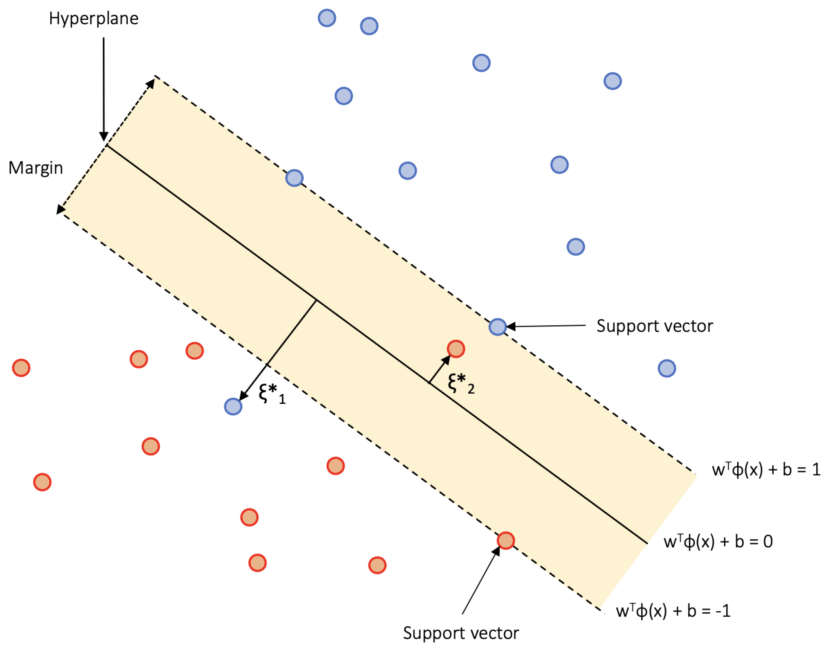
Support Vector Machine is a powerful supervised learning algorithm proposed by Cortes and Vapnik [23] in 1995. The core principle behind the SVM algorithm is to transform the input features into a higher-dimensional space using a process known as the kernel trick. Within this transformed space, the algorithm seeks to linearly separate the data classes using a high-dimensional surface, commonly referred to as a hyperplane, as illustrated in Figure 2.
Fundamentally, the SVM algorithm tackles a convex optimization problem, which can be effectively solved using the method of Lagrange multipliers. The mathematical complexity of this problem is considerably reduced by introducing the kernel notation. Kernel functions are instrumental in transforming the input data into the required higher-dimensional space, with the choice of kernel influencing the accuracy of the SVM model. Commonly employed kernel functions in SVM applications include
K l i n e a r ( x i , x j ) = γ x i x j ,
K p o l y n o m i a l ( x i , x j ) = ( γ x i x j + r ) d , γ > 0 ,
K R B F ( x i , x j ) = e x p ( γ x i x j 2 ) , γ > 0 ,
where K l i n e a r is the linear kernel, K p o l y n o m i a l is the polynomial kernel, and K R B F is the Radial Basis Function kernel.
In the context of the polynomial kernel, parameter γ acts as an inner product coefficient, d represents the degree of the polynomial, and r is a free parameter trading off the influence of higher-order versus lower-order terms.
For the RBF kernel, parameter γ determines the width of the RBF, controlling the degree of influence of a single training example, with lower values meaning far points influence the fit, and high values meaning close points influence the fit.
The SVM algorithm leverages these kernel functions to construct an optimal hyperplane that maximizes the margin between the classes in the feature space, thereby achieving superior classification performance. This technique is particularly beneficial when dealing with non-linear and high-dimensional data, enabling the SVM algorithm to handle a wide range of complex classification problems.

3. Study Area

3.1. Geologic Setting

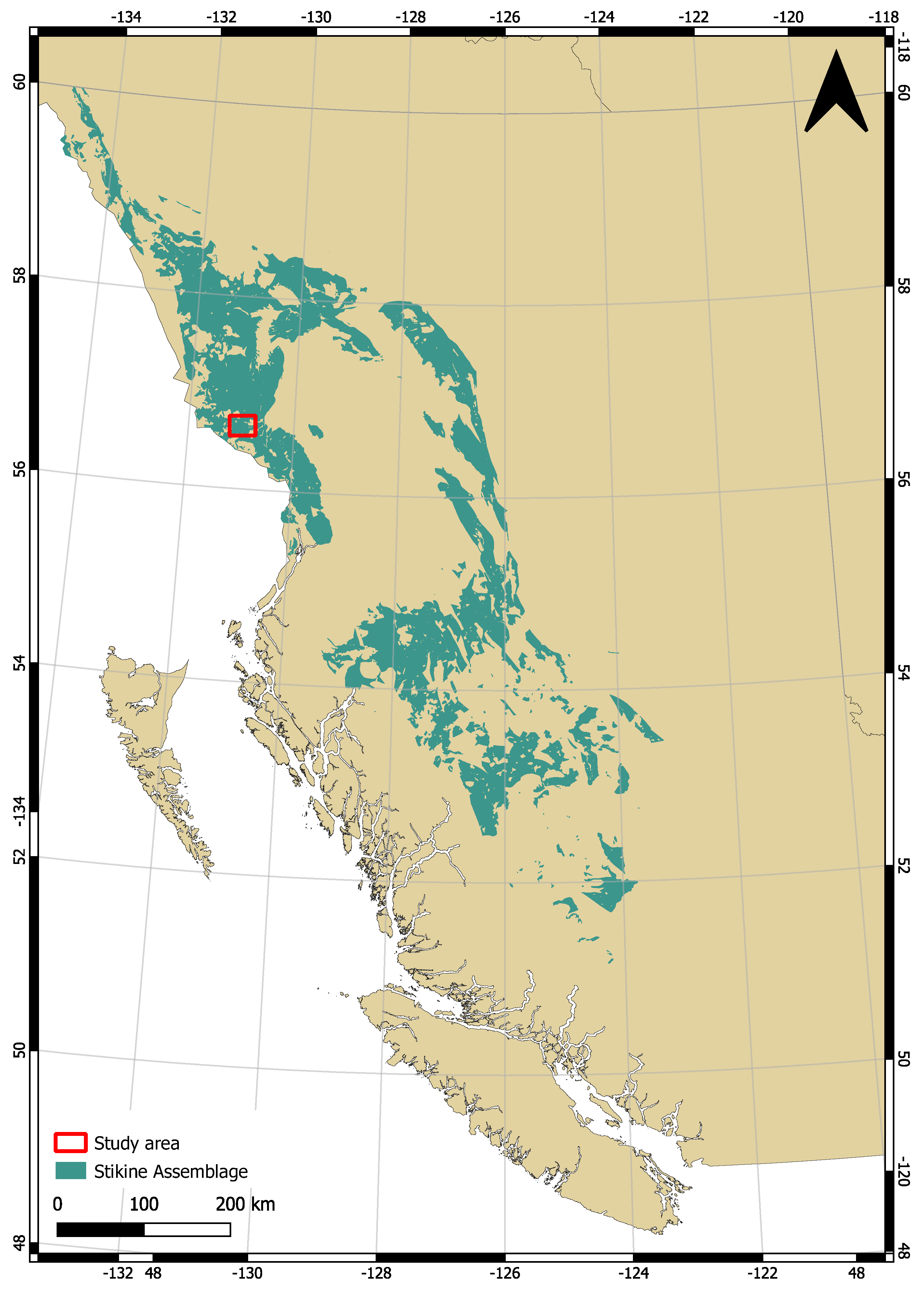
The area under study situated within the Stikine Terrane encompasses three distinct geological units, as illustrated in Figure 3. The most ancient of these formations is the Stikine Assemblage comprising deformed and metamorphosed marine sedimentary rocks, clastic sedimentary formations, and volcanic material, all dating back to the Upper Paleozoic epoch [24]. These primordial rocks lay the foundational geological context for the region.
Much of the study area is characterized by the substantial presence of variably deformed oceanic island arc complexes associated with the Triassic Stuhini and Jurassic Hazelton groups. The Stuhini Group predominantly comprises folded marine volcanic and sedimentary arc-related strata. These have undergone a certain level of alteration and low-grade metamorphism, marking significant geological transformations [24].
The Hazelton Group, on the other hand, consists of Early to Middle Jurassic subaerial and submarine volcanic and sedimentary rocks. This group is distinguished from the Stuhini Group by a discernible regional angular unconformity [24]. Patches of Quaternary basalts and localized volcanic activity have been recorded in the study area’s northern, southern, and northeastern regions.
The region also hosts mineralized Mesozoic plutonic bodies, the formation of which is correlated with significant regional metallogenic events. The Late Triassic Stikine Plutonic Suite, which spans 236–221 Ma, is associated with the emplacement of a mineralized pluton in the Cordillera [24,25]. The Texas Creek Plutonic Suite comprises two distinct magmatic events, each associated with a different style of mineralization. The first event occurred during the Early Jurassic, between 195 and 187 Ma, while the second was synchronous with the upper volcanic sequence of the Hazelton Group [24,25,26]. Older intrusions are linked to porphyry and gold-vein mineralizations, whereas younger intrusions are associated with exhalative mineralization [24].
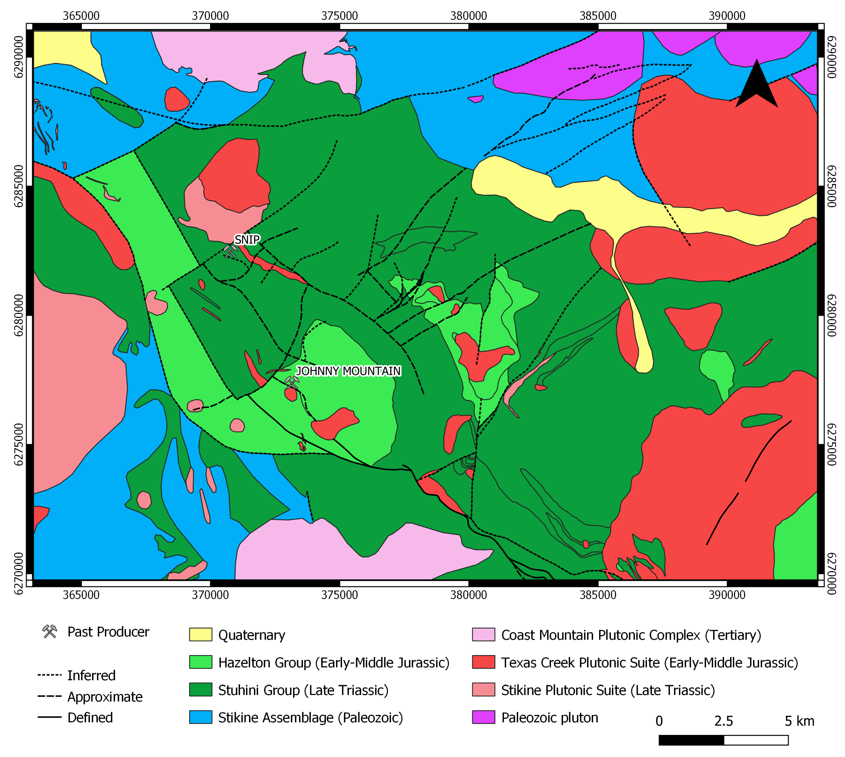
In terms of mineralogy, local deposits such as the Snip, Johnny Mountain (Stonehouse), or Inel deposits primarily contain vein-hosted gold, manifesting either as shear-veins or sulfide–quartz dilatant veins. As shown in Figure 4, mineralization within all three deposits occurs concurrently and co-locally with Early Jurassic porphyritic intrusions of the Texas Creek Plutonic Suite [27]. This spatial and temporal association of mineralized structures and intrusions establishes the occurrence of an Early Jurassic intrusion-related deformational and hydrothermal event within an extensional subvolcanic environment [27].

3.2. Conceptual Exploration Model

To delineate and prioritize areas prospective for epithermal Au deposits, we employed a mineral system approach described by McCuaig et al. [28]. This process involved defining the exploration criteria based on three critical factors:
  • The existence of potential Au source rocks.
  • The presence of a favorable geological setting (also referred to as traps).
  • The existence of clear pathways for the mineralization process.
Also, a total of seven spatial proxies were used to represent the defined exploration criteria, each corresponding to a vital element of the exploration model (Table 1).

4. Methodology

4.1. Data Preparation

4.1.1. Training Dataset

To create a robust and effective training dataset, we utilized the known mineral occurrences depository (MINFILE) maintained by the BC Geological Survey [29]. These locations, categorized as either deposit (mineral occurrence) or non-deposit, were classified as “prospective” and “non-prospective”, respectively. A binary system was employed, attributing a value of 1 to deposit locations and a value of 0 to non-deposit locations.
We carefully selected 18 mineral occurrences within our study area to function as training deposit locations (refer to Appendix A). Our selection criteria were as follows:
  • Au must be listed as the primary commodity;
  • The occurrence must be categorized as an epithermal deposit (i.e., vein type);
  • The occurrence must be an advanced exploration project (i.e., prospects and past producers).
The selection of non-deposit locations was dictated by their geographic distance from deposit locations and the absence of Au as a top three commodity. Point pattern analysis enabled us to define an optimal distance parameter of 2000 m, demonstrating a 78% probability of discovering a neighboring deposit (Figure 5) [13]. Following this selection process, we were left with 19 non-deposit occurrences (refer to Appendix B). It is worth noting that the study area behaves like a vast epithermal–porphyry system. This means that deposit and non-deposit locations might exhibit similar geospatial signatures, posing a challenge for distinct classification.
However, our training dataset maintained balance (i.e., the count of non-deposit locations closely mirrors that of deposit locations). This allowed us the avoidance of further reduction in or alteration of non-prospective mineral occurrences from our non-deposit training dataset with additional filters.

4.1.2. Input Dataset

The methodology of this study harnesses both privately sourced and publicly accessible datasets. These encompass geological, geophysical, and remote sensing data. Our geological information was culled from the 1:50,000 scale geological maps provided by the British Columbia Geological Survey [30,31].
Geophysical data, particularly magnetic survey data, were acquired from the Canadian Aeromagnetic Database [32]. We leveraged the ASTER Level 1 Precision Terrain Corrected Registered At-Sensor Radiance (L1T) data [33] for remote sensing data due to their accurate and reliable representation of the study area.
In addition to public data, we incorporated geochemical data (i.e., soil samples) provided by Seabridge Gold Inc. These samples are the result of surveys conducted by private companies spanning 30 years from 1981 to 2011. These disparate datasets, when combined, offer a comprehensive view of the study area and enhance the precision of our machine learning models.

4.1.3. Evidential Features

To encapsulate the exploration criteria for epithermal Au deposits within the Iskut property, we utilized our input dataset to derive predictor maps. These maps, as outlined in our exploration model, represent critical components in our search for prospective Au deposits. Following the methodology proposed by Carranza [34] in 2009, we determined a cell size unit of 50 m × 50 m for our predictor maps and MPM. This pixel size was specifically chosen to correspond appropriately to the spatial resolution of the dataset in use and to ensure that only one deposit is captured within a single pixel. A detailed discussion on predictor maps, including aspects such as distance to intrusions, distance to faults, favorable host rock, Au geochemical anomaly, principal components, magnetic first vertical derivative, argillic alteration, iron oxides alteration, phyllic alteration, propylitic alteration, and silica alteration which are used in this benchmark study can be found in Lachaud et al. [13].
In the study area, Mesozoic intrusive bodies serve as potential sources of Au, with mineralized veins often linked to a brittle–ductile deformation. As a result, we generated maps at 500 m intervals showing distance to Mesozoic intrusions (i.e., Stikine Plutonic Suite and Texas Creek Plutonic Suite) and distance to structural features (i.e., fault trace and fold axis trace). In terms of geology, we assigned a “favorable” host rock category to units such as the Stuhini Group and the Hazelton Group, which host deposits in the area. In contrast, all other units were classified as “non-favorable” host rock.
Magnetic surveys can play a crucial role in uncovering concealed structural features. We employed the first vertical derivative of the magnetic survey to emphasize near-surface structures.
Geochemical data, providing insights into rock types, alteration minerals, and anomalous concentrations, are of immense value in mineral exploration. We used the following elements to produce predictor maps: Ag, Au, As, Ba, Co, Cu, Fe, Mn, Mo, Pb, Sb, Zn. To standardize the data, we used a centered log-ratio (clr) transformation [35], followed by a principal components analysis (PCA) on the adjusted dataset. Geological processes, including differentiation, alteration, mineralization, and weathering, can be characterized by distinct principal components [36]. The clr-transformed Au values and the first and second principal components (representing potential metal associations and enrichment or depletion, respectively) were interpolated over the study area using the Inverse Distance Weighted (IDW) algorithm. Considering our study’s exploratory and benchmark nature, the IDW was chosen for its relative simplicity and the satisfactory results it has been found to provide in similar geospatial applications. By employing a straightforward weighted average, this method met the requirements of our study without the need for additional assumptions associated with more advanced techniques such as kriging.
We employed ASTER data to map prevalent alteration minerals and hydrothermal alteration. We generated five maps using band ratios and relative absorption band depth methods, allowing the mapping of argillic, iron oxides, phyllic, propylitic, and silica alterations.

4.2. Model Training

To develop the most effective models for predicting the location of Au mineral deposits, we employed a comprehensive parameter tuning process for both RF and SVM models.
The Random Forest model parameters include the number of decision trees (k) and the number of variables (m) randomly sampled at each split node. Although RF shows relative insensitivity to the number of trees in the forest, we conducted a detailed analysis to ascertain an optimal number, finally settling on k = 1000 . As the number of trees in the forest increases, the model’s generalization error tends to stabilize [14,20], thus reducing the likelihood of overfitting. We varied m between 2 and 14, covering a spectrum of model configurations for our evaluation process.
The Support Vector Machine models offer a more intricate set of parameters, as we utilized three kernel functions: l i n e a r , p o l y n o m i a l , and R a d i a l B a s i s F u n c t i o n ( R B F ) , each with its unique set of tunable parameters.
With its simplicity, the linear kernel offers fewer chances for overfitting and serves as an excellent starting point for tuning. The polynomial kernel has additional parameters, including the degree of the polynomial (d), a scaling factor ( γ ), and a bias term ( c o e f 0 ). The degree parameter dictates the complexity of the decision boundary, with higher values potentially leading to overfitting, making its tuning crucial. γ and c o e f 0 control the shape and position of the decision boundary, offering an extra layer of precision to the model.
The RBF kernel, with parameters C (regularization parameter) and γ (kernel coefficient), adds flexibility to our models. The C parameter mediates the trade-off between achieving the correct classification of training examples and maximizing the decision function’s margin. Simultaneously, the gamma parameter defines the influence extent of a single training example.
We defined a search grid for each SVM parameter to navigate the parameter space efficiently. The grid served as a systematic framework for tweaking the parameters and discovering the optimal configurations. The best parameters for each kernel were then selected based on their performance, as detailed in Table 2.

4.3. Model Evaluation

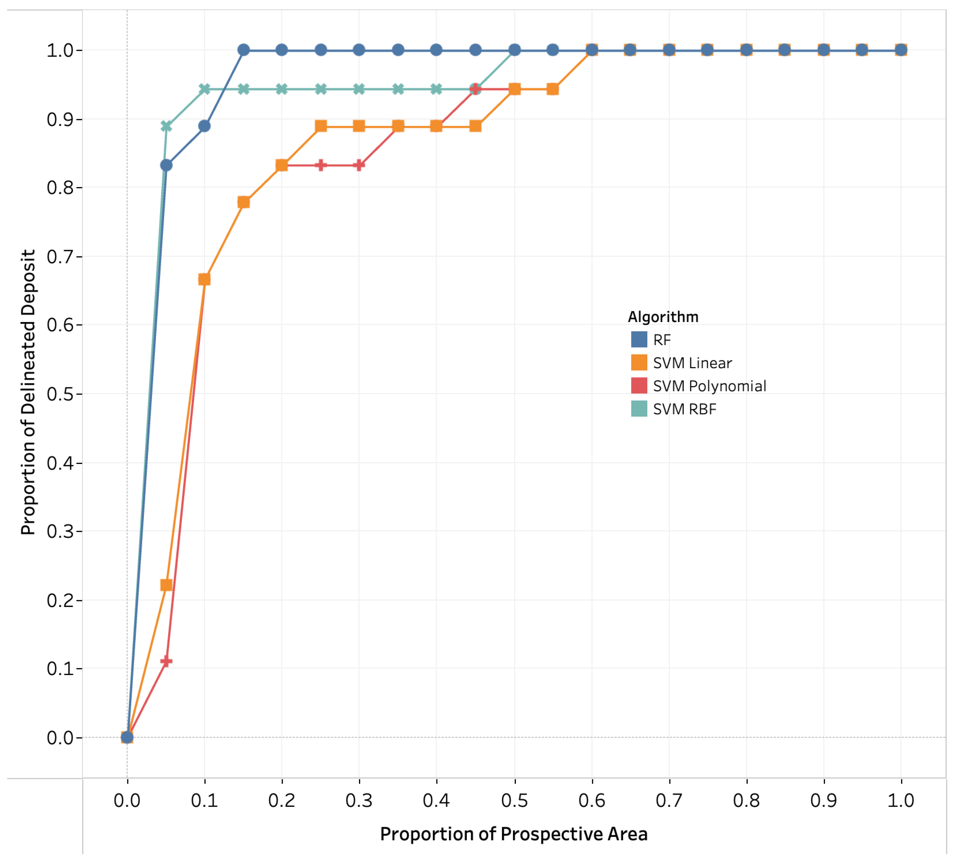
There are two methods to evaluate the importance of evidential features in a model: distant approximations (wrappers) and integrated approximation (embedded). RF has an embedded method for calculating the significance of features by calculating each evidential feature’s decrease in mean square error (MSE). In contrast, SVM is a “black box” technique and does not provide information about the role of features in predictive modeling. The importance of evidential features in the RF model was scaled between 0 and 100. Each prediction is represented by a floating value between 0 and 1, which denotes the probability of an Au mineral deposit occurrence. Predictions with a value higher than 0.5 are classified as prospective, whereas values below 0.5 are classified as non-prospective. Using that classification scheme, we calculated a series of statistical indices to assess the predictive accuracy of the MPM: overall accuracy, kappa index, sensitivity, and specificity. The Receiver Operating Characteristic (ROC) curve is a graphic representation of the performance of a binary classification system. The curve is generated by plotting sensitivity (also known as true positive rate, TPR) against false positive rate (FPR, given by 1-specificity) at varying thresholds [37]. The threshold determines the discrimination rule for the predictive results; cells with a value higher or lower than the threshold are classified as “deposit” or “non-deposit”, respectively. The closer the ROC curve is toward the upper left corner, the better the model performs. The overall performance of the resulting mineral prospectivity map can be evaluated with a success rate curve. The success rate curve is computed by reclassifying the predictive map according to different thresholds of an areal percentage of prospective zones and calculating the proportion of deposit locations delineated in those prospective zones [18].

5. Results

5.1. Sensitivity Analysis

The chosen parameters for model training critically influence the robustness and generalization capabilities of machine learning methods, thus shaping the predictive accuracy. We used the Root Mean Square Error (RMSE) to identify the optimal values for various parameters across the different models, validated through 10-fold cross-validation.
Table 3 illustrates the variation in accuracy among the algorithms used in the 10-fold cross-validation, all employing optimized parameters. Among the studied models, the SVM with a Radial Basis Function kernel ( S V M R B F ) achieved the lowest mean RMSE (0.306), while the RF model recorded the highest value (0.388). Remarkably, SVM with a linear kernel ( S V M l i n e a r ) exhibited the most stable prediction, recording the lowest minimum (0.149), maximum (0.504), and standard deviation (0.103) across all folds.
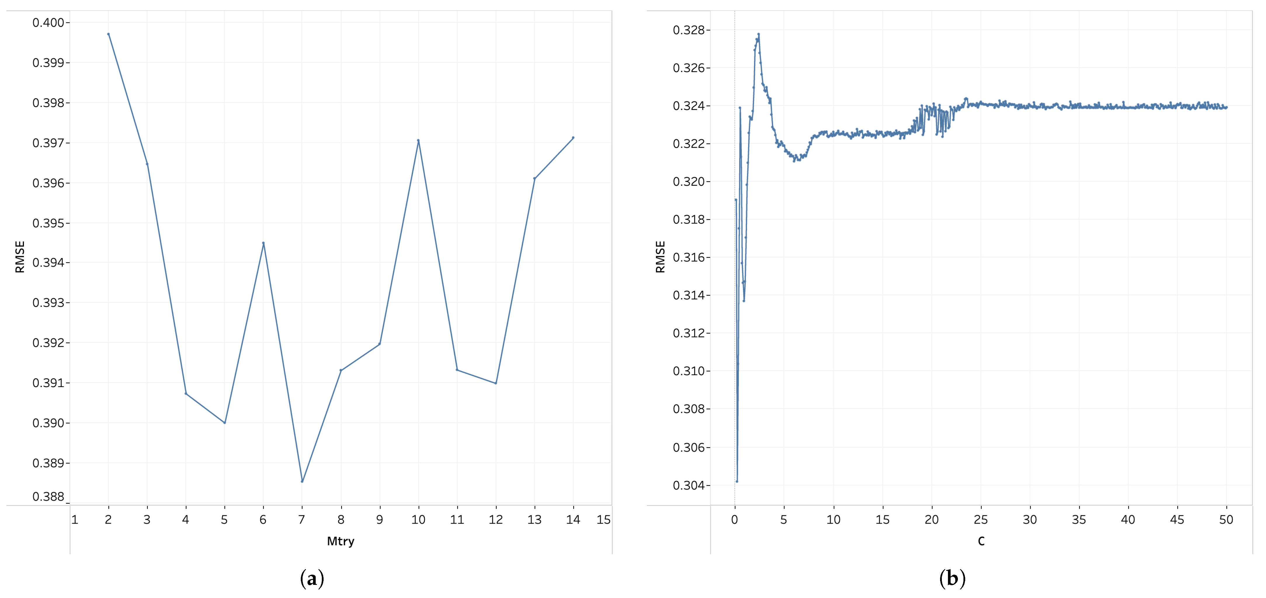
Figure 6 and Figure 7 display the RMSE variation for different parameter values within each model. Given that the RF and S V M l i n e a r have only one parameter (with RF’s second parameter k fixed, as discussed in Section 4.2), their behavior differs from that of S V M R B F and SVM with a polynomial kernel ( S V M p o l y ), which contain two and three parameters, respectively.
The RF’s parameter variation has a negligible impact on the classification results, underscoring its stability and insensitivity to parameter configuration. The S V M l i n e a r shows convergence for C values above 24, suggesting that with a large enough C, the model stabilizes (Figure 6).
In contrast, S V M R B F and S V M p o l y exhibit complex RMSE variations. For S V M R B F , the sigma parameter greatly influences performance, while the cost parameter’s impact is limited. Optimal RMSE values were observed with costs above 1 and sigma values lower than 0.15. Similarly, for S V M p o l y , the scale parameter strongly influences the model’s performance, with the minimum RMSE values attained at a degree d of 1, a cost lower than 2, and a scale lower than 0.35 (Figure 7).
The robustness of the RF model is ascribed to the randomness incorporated in its training data selection, reducing tree correlation and enhancing generalization capabilities [20]. Further, by randomly choosing features for each tree, the model minimizes overfitting [20,22].

5.2. Performance Assessment of the Predictive Models

In the context of overall accuracy, all the SVM models demonstrated superior performance over the Random Forest (RF) model, with accuracies of 89%, 97%, and 89% for the linear kernel ( S V M linear ), Radial Basis Function kernel ( S V M RBF ), and polynomial kernel ( S V M poly ), respectively, as detailed in Table 4. Furthermore, an examination of the ROC probability curves in Figure 8 reveals that the RF model is consistently outperformed by all three SVM variants.
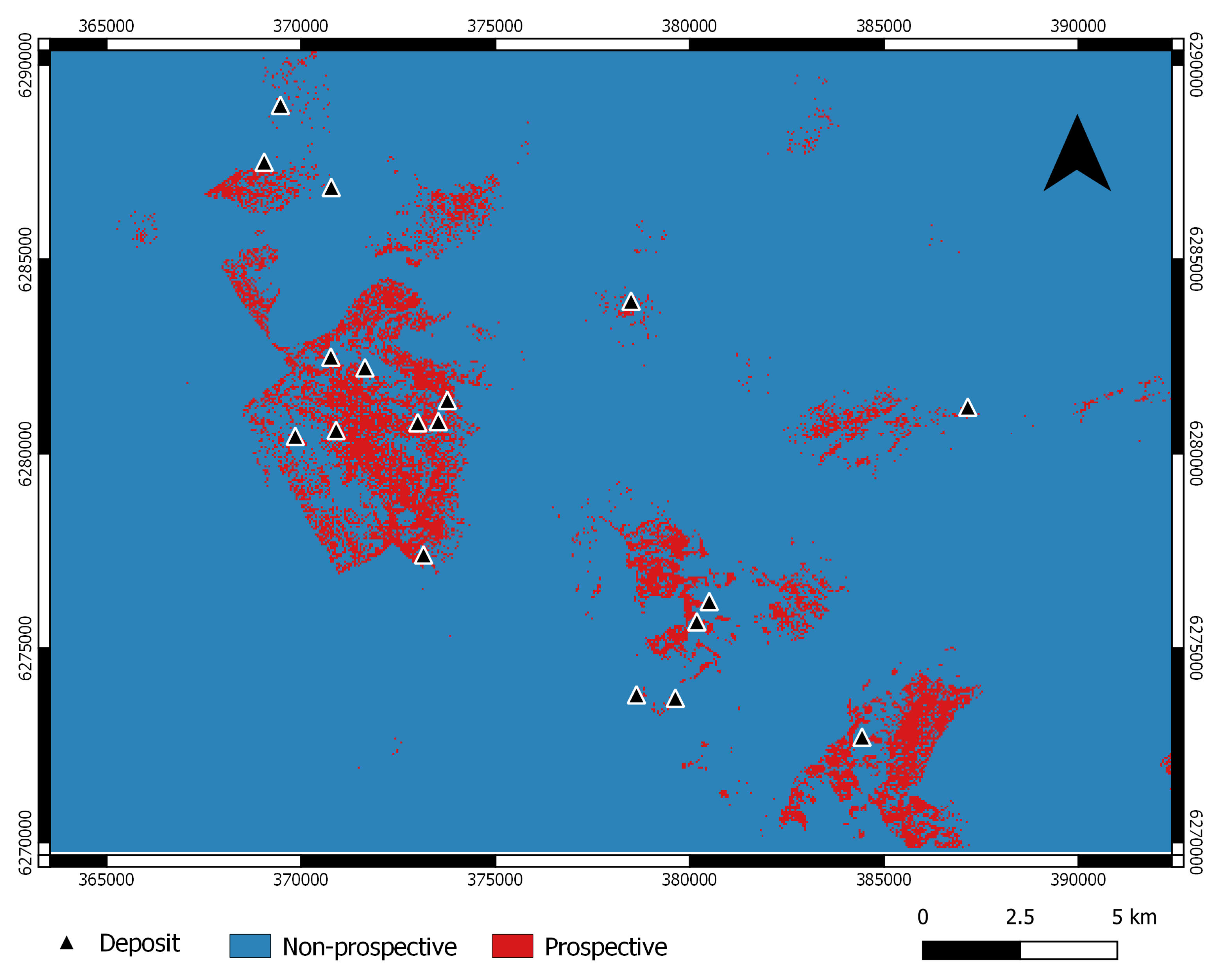
However, despite these superior accuracies, the SVM models fell short in delineating training deposits within a small region (Figure 9), a vital aim of mineral prospectivity mapping.
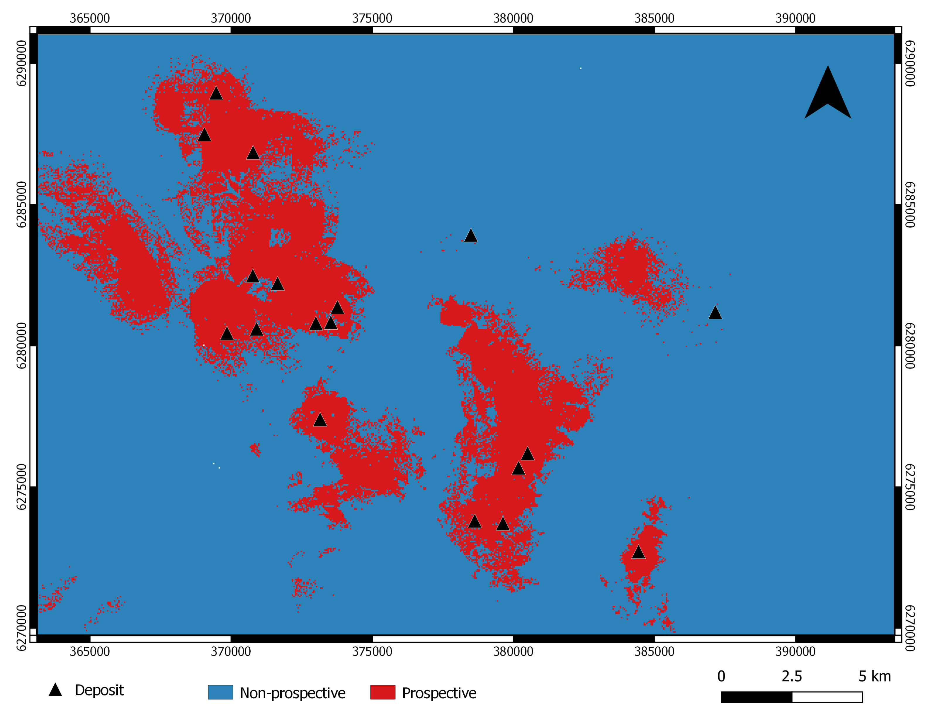
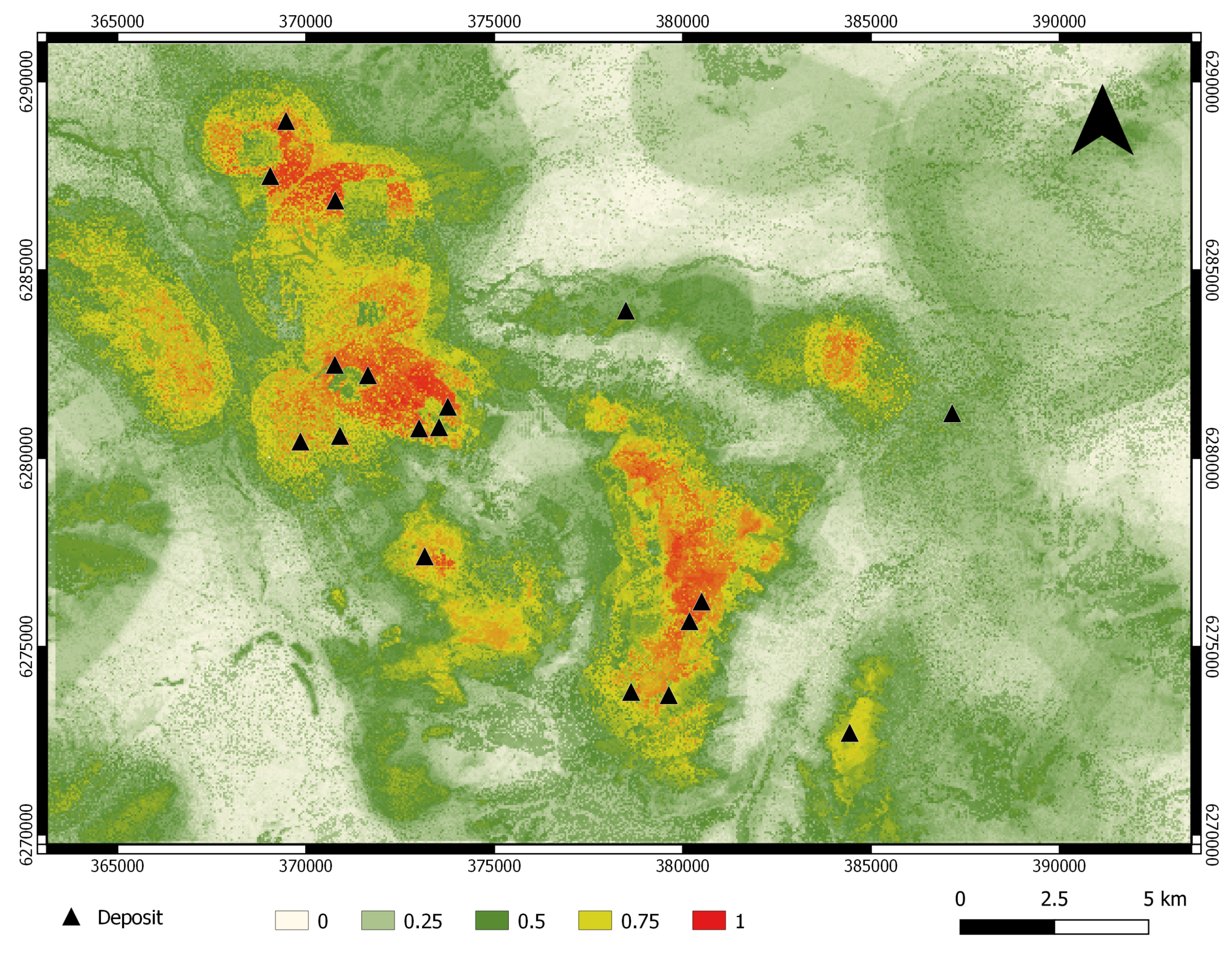
Although the RF model’s accuracy was moderately lower (78%), the RF-generated mineral prospectivity map required only 15% of the total area to delineate all the deposits (Figure 10). This compact area, contrasted with the 50%–60% area required for SVM-generated maps, led us to choose the RF mineral prospectivity map as the final predictive map for epithermal Au deposit potential (Figure 11).
Despite employing a 10-fold cross-validation to mitigate overfitting, the high accuracy indices and optimal ROC curves, but poor success-rate curves (Figure 12), suggest an overfitting issue in the SVM models. The smaller training dataset size compared to the studies by Rodriguez-Galiano et al. [14] and Sun et al. [20] likely exacerbates this issue, underscoring the need for larger training datasets for SVM to mitigate overfitting.

5.3. Feature Relative Importance

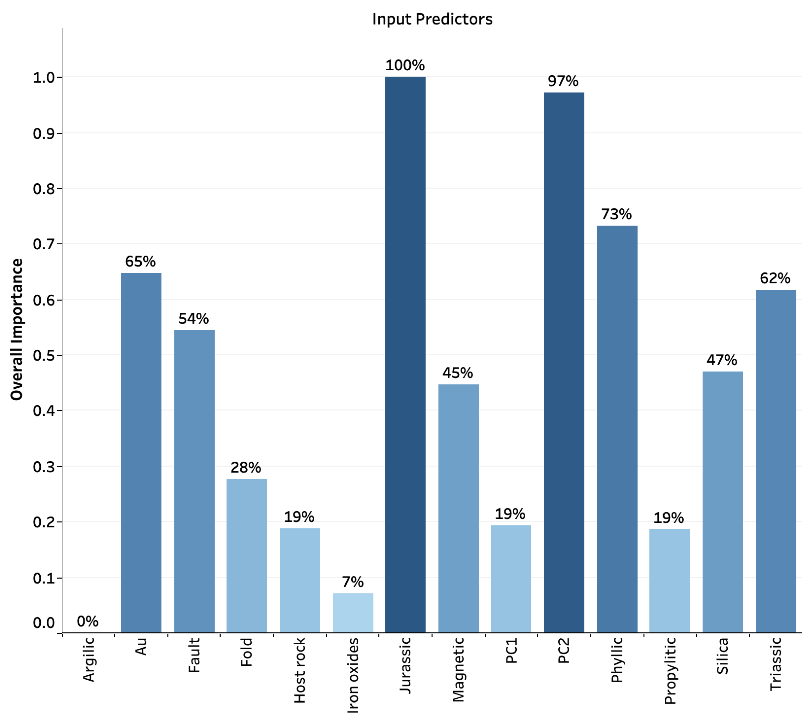
In contrast with SVM, RF has an embedded assessment of input predictor importance, thereby identifying crucial exploration criteria (Figure 13).
The proximity to Jurassic intrusions emerged as the top-ranked feature, surpassing the importance of proximity to Triassic intrusions. Therefore, the primary source of mineralized hydrothermal fluids for our training deposit locations likely originates from the Texas Creek Plutonic Suite (Early to Middle Jurassic) rather than the Stikine Plutonic Suite (Late Triassic).
The critical chemical trap proxies include PC2, Au anomalies, phyllic, and silica alterations, indicating associations with high-temperature, acidic fluids. Thus, it suggests that Au mineralization is linked with quartz veining, implying a potential deep porphyry system presence in the area. The host rocks predictor map and other alteration types, though useful as chemical trap proxies, are of minor importance in the model.
The proximity to the fault predictor map is more influential than the proximity to the fold predictor map. Consequently, for epithermal Au deposit exploration in the region, faulting serves as a superior criterion compared to folding.

6. Conclusions

The comparative analysis of Support Vector Machine (SVM) and Random Forest (RF) for mineral prospectivity mapping of epithermal Au deposits has yielded significant insights from three dimensions: sensitivity to configuration, interpretability, and predictive accuracy of the models. Our study distinguishes itself by operating with a relatively small training dataset (<20 deposits) and adopting a mineral system approach encompassing all key processes—source, transport, trap, and deposition—critical for ore formation. In total, 14 predictor maps were used to represent these processes.
Our sensitivity analysis emphasized the less pronounced sensitivity of RF to variations in parameters than SVM, irrespective of the kernel function employed in the latter. This finding underscores the impressive stability of RF, making it an advantageous choice for mineral prospectivity mapping, especially in cases of smaller datasets.
The interpretability of RF was another key aspect of our study. The model elucidated the relative importance of the input predictors, identifying proximity to Jurassic intrusions as the top-ranked feature, followed by multi-element geochemical anomalies and phyllic alteration. Additionally, the proximity to faults was identified as the sixth most important feature, indicating the importance of geological structures in the mineralization process.
The predictive accuracy of the models unveiled the superior performance of SVM models in terms of training accuracy indices. All SVM models outperformed the RF model in this regard, with accuracies of 89% ( S V M l i n e a r ), 97% ( S V M R B F ), and 89% ( S V M p o l y ). Similarly, the SVM models excelled in the ROC curve analysis. However, the seeming perfection of SVM model accuracy may be indicative of overfitting, possibly due to the limited size of the training dataset.
The RF model, despite its moderate accuracy of 78%, proved more efficient in practical terms, delineating all deposits within just 15% of the total study area. Consequently, it was chosen as the most effective predictive model for this study.

Author Contributions

Conceptualization, A.L., I.M. and M.A.; methodology, A.L. and I.M.; validation, A.L. and I.M.; formal analysis, A.L.; investigation, A.L.; data curation, A.L.; writing—original draft preparation, A.L.; writing, review and editing, A.L., M.A. and I.M.; supervision, I.M. All authors have read and agreed to the published version of the manuscript.

Funding

This research received no external funding.

Data Availability Statement

Original datasets used in this study can be found at the following public online data repositories: https://catalogue.data.gov.bc.ca/dataset/minfile-mineral-occurrence-database (accessed on 30 April 2023), hosted by the Government of British Columbia; https://catalogue.data.gov.bc.ca/dataset/bedrock-geology (accessed on 30 April 2023), hosted by the Government of British Columbia; https://www2.gov.bc.ca/gov/content/industry/mineral-exploration-mining/british-columbia-geological-survey/publications/geofiles (accessed on 30 April 2023), hosted by the Government of British Columbia; http://gdr.agg.nrcan.gc.ca/gdrdap/dap/index-eng.php?db_project_no=10011 (accessed on 30 January 2022), hosted by Natural Resources Canada; https://earthexplorer.usgs.gov (accessed on 30 January 2022), hosted by USGS.

Conflicts of Interest

The funders had no role in the design of the study; in the collection, analyses, or interpretation of data; in the writing of the manuscript, or in the decision to publish the results.

Appendix A

Table A1. Deposit locations from the mineral occurrences depository (MINFILE). The coordinates are in Universal Transverse Mercator (UTM) coordinate system (NAD83/zone 9N).
MINFILE #NAMESTATUSUTM NORTHUTM EAST
104B 077BRONSON SLOPEDeveloped Prospect6,282,211371,642
104B 089SNIP NORTH-EAST ZONEProspect6,286,850370,775
104B 107JOHNNY MOUNTAINPast Producer6,277,401373,149
104B 113INELDeveloped Prospect6,275,679380,178
104B 116TAMI (BLUE RIBBON)Prospect6,272,714384,430
104B 138KHYBER PASSProspect6,273,715379,627
104B 204WARATAH 6Prospect6,283,926378,489
104B 250SNIPPast Producer6,282,486370,764
104B 264C3 (REG)Prospect6,280,600370,900
104B 300BRONSONProspect6,281,374373,763
104B 356GORGEProspect6,287,500369,050
104B 357GREGORProspect6,288,962369,467
104B 537MYSTERYProspect6,281,200387,150
104B 557AKProspect6,276,200380,500
104B 563CE CONTACTProspect6,280,800373,000
104B 567SMCProspect6,280,450369,850
104B 571CEProspect6,280,829373,529
104B 685KHYBER WESTProspect6,273,802378,627

Appendix B

Table A2. The selected non-deposit location from the mineral occurrences depository (MINFILE). The coordinates are in Universal Transverse Mercator (UTM) coordinate system (NAD83/zone 9N).
MINFILE #NAMESTATUSUTM NORTHUTM EAST
104B 005CRAIG RIVERShowing6,276,177366,697
104B 205HANDELShowing6,281,905376,693
104B 206WOLVERINEShowing6,277,250377,150
104B 256WOLVERINE (INEL)Showing6,277,063383,766
104B 268HANGOVER TRENCHShowing6,275,185369,738
104B 272DAN 2Showing6,271,824375,475
104B 292GIM (ZONE 1)Showing6,281,770383,605
104B 305MILLShowing6,272,879363,417
104B 306NORTH CREEKShowing6,275,031368,709
104B 324IAN 4Showing6,286,725379,485
104B 326CAM 9Showing6,279,635391,709
104B 327CAM SOUTHShowing6,279,579392,696
104B 331IAN 8Showing6,286,038383,655
104B 362KIRK MAGNETITEShowing6,276,565389,635
104B 368ELMERShowing6,275,780391,286
104B 377ROCK AND ROLLDeveloped Prospect6,288,261363,286
104B 416IAN 6 SOUTHShowing6,286,900382,200
104B 500KRL-FORRESTShowing6,288,950393,400
104B 536ANDYShowing6,278,300385,825

References

  1. Bonham-Carter, G. Geographic Information Systems for Geoscientists: Modelling with GIS; Number 13; Elsevier: Amsterdam, The Netherlands, 1994. [Google Scholar]
  2. Carranza, E.; Hale, M.; Faassen, C. Selection of coherent deposit-type locations and their application in data-driven mineral prospectivity mapping. Ore Geol. Rev. 2008, 33, 536–558. [Google Scholar] [CrossRef]
  3. Harris, D.; Zurcher, L.; Stanley, M.; Marlow, J.; Pan, G. A comparative analysis of favorability mappings by weights of evidence, probabilistic neural networks, discriminant analysis, and logistic regression. Nat. Resour. Res. 2003, 12, 241–255. [Google Scholar] [CrossRef]
  4. Joly, A.; Porwal, A.; McCuaig, T.C. Exploration targeting for orogenic gold deposits in the Granites-Tanami Orogen: Mineral system analysis, targeting model and prospectivity analysis. Ore Geol. Rev. 2012, 48, 349–383. [Google Scholar] [CrossRef]
  5. Harris, J.; Wilkinson, L.; Heather, K.; Fumerton, S.; Bernier, M.; Ayer, J.; Dahn, R. Application of GIS processing techniques for producing mineral prospectivity maps—A case study: Mesothermal Au in the Swayze Greenstone Belt, Ontario, Canada. Nat. Resour. Res. 2001, 10, 91–124. [Google Scholar] [CrossRef]
  6. Brown, W.M.; Gedeon, T.; Groves, D.; Barnes, R. Artificial neural networks: A new method for mineral prospectivity mapping. Aust. J. Earth Sci. 2000, 47, 757–770. [Google Scholar] [CrossRef]
  7. Abedi, M.; Norouzi, G.H.; Bahroudi, A. Support vector machine for multi-classification of mineral prospectivity areas. Comput. Geosci. 2012, 46, 272–283. [Google Scholar] [CrossRef]
  8. Geranian, H.; Tabatabaei, S.H.; Asadi, H.H.; Carranza, E.J.M. Application of discriminant analysis and support vector machine in mapping gold potential areas for further drilling in the Sari-Gunay gold deposit, NW Iran. Nat. Resour. Res. 2016, 25, 145–159. [Google Scholar] [CrossRef]
  9. Shabankareh, M.; Hezarkhani, A. Application of support vector machines for copper potential mapping in Kerman region, Iran. J. Afr. Earth Sci. 2017, 128, 116–126. [Google Scholar] [CrossRef]
  10. Carranza, E.J.M.; Laborte, A.G. Data-driven predictive mapping of gold prospectivity, Baguio district, Philippines: Application of Random Forests algorithm. Ore Geol. Rev. 2015, 71, 777–787. [Google Scholar] [CrossRef]
  11. Carranza, E.J.M.; Laborte, A.G. Data-driven predictive modeling of mineral prospectivity using random forests: A case study in Catanduanes Island (Philippines). Nat. Resour. Res. 2016, 25, 35–50. [Google Scholar] [CrossRef]
  12. Harris, J.; Grunsky, E.; Behnia, P.; Corrigan, D. Data-and knowledge-driven mineral prospectivity maps for Canada’s North. Ore Geol. Rev. 2015, 71, 788–803. [Google Scholar] [CrossRef]
  13. Lachaud, A.; Marcus, A.; Vučetić, S.; Mišković, I. Study of the Influence of Non-Deposit Locations in Data-Driven Mineral Prospectivity Mapping: A Case Study on the Iskut Project in Northwestern British Columbia, Canada. Minerals 2021, 11, 597. [Google Scholar] [CrossRef]
  14. Rodriguez-Galiano, V.; Sanchez-Castillo, M.; Chica-Olmo, M.; Chica-Rivas, M. Machine learning predictive models for mineral prospectivity: An evaluation of neural networks, random forest, regression trees and support vector machines. Ore Geol. Rev. 2015, 71, 804–818. [Google Scholar] [CrossRef]
  15. Zuo, R.; Carranza, E.J.M. Support vector machine: A tool for mapping mineral prospectivity. Comput. Geosci. 2011, 37, 1967–1975. [Google Scholar]
  16. De Boissieu, F.; Sevin, B.; Cudahy, T.; Mangeas, M.; Chevrel, S.; Ong, C.; Rodger, A.; Maurizot, P.; Laukamp, C.; Lau, I.; et al. Regolith-geology mapping with support vector machine: A case study over weathered Ni-bearing peridotites, New Caledonia. Int. J. Appl. Earth Obs. Geoinf. 2018, 64, 377–385. [Google Scholar] [CrossRef]
  17. Kuhn, S.; Cracknell, M.J.; Reading, A.M. Lithologic mapping using Random Forests applied to geophysical and remote-sensing data: A demonstration study from the Eastern Goldfields of Australia. Geophysics 2018, 83, B183–B193. [Google Scholar] [CrossRef]
  18. Rodriguez-Galiano, V.; Mendes, M.P.; Garcia-Soldado, M.J.; Chica-Olmo, M.; Ribeiro, L. Predictive modeling of groundwater nitrate pollution using Random Forest and multisource variables related to intrinsic and specific vulnerability: A case study in an agricultural setting (Southern Spain). Sci. Total Environ. 2014, 476, 189–206. [Google Scholar] [CrossRef] [PubMed]
  19. Singh, S.K.; Srivastava, P.K.; Gupta, M.; Thakur, J.K.; Mukherjee, S. Appraisal of land use/land cover of mangrove forest ecosystem using support vector machine. Environ. Earth Sci. 2014, 71, 2245–2255. [Google Scholar] [CrossRef]
  20. Sun, T.; Chen, F.; Zhong, L.; Liu, W.; Wang, Y. GIS-based mineral prospectivity mapping using machine learning methods: A case study from Tongling ore district, eastern China. Ore Geol. Rev. 2019, 109, 26–49. [Google Scholar] [CrossRef]
  21. Ho, T.K. Random decision forests. In Proceedings of the 3rd International Conference on Document Analysis and Recognition, Montreal, QC, Canada, 14–16 August 1995; IEEE: Piscataway, NJ, USA, 1995; Volume 1, pp. 278–282. [Google Scholar]
  22. Breiman, L. Random forests. Mach. Learn. 2001, 45, 5–32. [Google Scholar] [CrossRef] [Green Version]
  23. Cortes, C.; Vapnik, V. Support-vector networks. Mach. Learn. 1995, 20, 273–297. [Google Scholar] [CrossRef]
  24. Macdonald, A.J.; Lewis, P.D.; Thompson, J.F.; Nadaraju, G.; Bartsch, R.; Bridge, D.J.; Rhys, D.A.; Roth, T.; Kaip, A.; Godwin, C.I.; et al. Metallogeny of an early to middle Jurassic arc, Iskut river area, northwestern British Columbia. Econ. Geol. 1996, 91, 1098–1114. [Google Scholar] [CrossRef]
  25. Logan, J.M.; Mihalynuk, M.G. Tectonic controls on early Mesozoic paired alkaline porphyry deposit belts (Cu-Au±Ag-Pt-Pd-Mo) within the Canadian Cordillera. Econ. Geol. 2014, 109, 827–858. [Google Scholar] [CrossRef]
  26. Burgoyne, A.; Giroux, G. Mineral Resource Estimate—Bronson Slope Deposit; Technical Report Prepared for Skyline Gold Corporation; Skyline Gold Corporation: Vancouver, BC, Canada, 2008. [Google Scholar]
  27. Rhys, D.A. Geology of the Snip Mine, and Its Relationship to the Magmatic and Deformational History of the Johnny Mountain Area, Northwestern British Columbia. Ph.D. Thesis, University of British Columbia, Vancouver, BC, Canada, 1993. [Google Scholar]
  28. McCuaig, T.C.; Beresford, S.; Hronsky, J. Translating the mineral systems approach into an effective exploration targeting system. Ore Geol. Rev. 2010, 38, 128–138. [Google Scholar] [CrossRef]
  29. MINFILE Mineral Occurrence Database. Available online: https://catalogue.data.gov.bc.ca/dataset/minfile-mineral-occurrence-database (accessed on 30 April 2023).
  30. Bedrock Geology. Available online: https://catalogue.data.gov.bc.ca/dataset/bedrock-geology (accessed on 30 April 2023).
  31. GeoFiles. Available online: https://www2.gov.bc.ca/gov/content/industry/mineral-exploration-mining/british-columbia-geological-survey/publications/geofiles (accessed on 30 April 2023).
  32. Geophysical Data Portal. Available online: http://gdr.agg.nrcan.gc.ca/gdrdap/dap/index-eng.php?db_project_no=10011 (accessed on 30 January 2022).
  33. USGS Earth Explorer. Available online: https://earthexplorer.usgs.gov (accessed on 30 January 2022).
  34. Carranza, E.J.M. Objective selection of suitable unit cell size in data-driven modeling of mineral prospectivity. Comput. Geosci. 2009, 35, 2032–2046. [Google Scholar] [CrossRef]
  35. Aitchison, J. The statistical analysis of compositional data. J. R. Stat. Soc. Ser. B (Methodol.) 1982, 44, 139–160. [Google Scholar] [CrossRef]
  36. Grunsky, E.C. The interpretation of geochemical survey data. Geochem. Explor. Environ. Anal. 2010, 10, 27–74. [Google Scholar] [CrossRef]
  37. Nykänen, V.; Lahti, I.; Niiranen, T.; Korhonen, K. Receiver operating characteristics (ROC) as validation tool for prospectivity models—A magmatic Ni–Cu case study from the Central Lapland Greenstone Belt, Northern Finland. Ore Geol. Rev. 2015, 71, 853–860. [Google Scholar] [CrossRef]
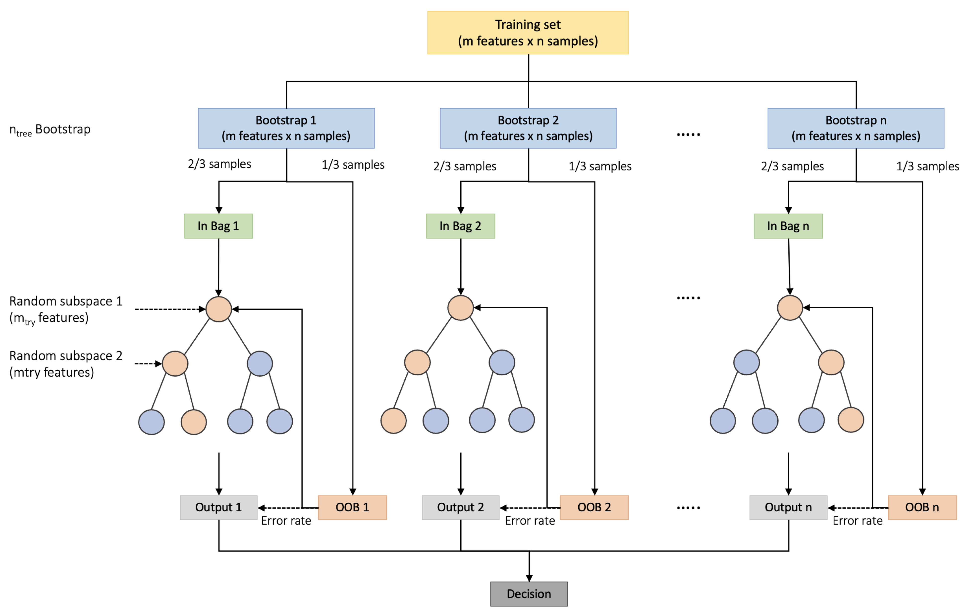
Figure 1. Generalized RF Structure.
Minerals 13 01073 g001
Figure 2. Classification of Data by SVM with Non-separable Features.
Minerals 13 01073 g002
Figure 3. Regional Map Showing the Study Area within Stikine Assemblage and British Columbia.
Minerals 13 01073 g003
Figure 4. Geology of the Study Area [13].
Minerals 13 01073 g004
Figure 5. Locations of Deposit and Non-deposit Training Data Points [13].
Minerals 13 01073 g005
Figure 6. Classification error for different parameters of the RF (a) and SVMlinear (b).
Minerals 13 01073 g006
Figure 7. Classification error for different parameters of the S V M R B F (a) and S V M p o l y with d = 1 (b), d = 2 (c), d = 3 (d), d = 4 (e), and d = 5 (f).
Minerals 13 01073 g007
Figure 8. ROC curves for Tested SVM and RF models.
Minerals 13 01073 g008
Figure 9. SVM Mineral Prospectivity Map Showing the delineated prospective zone using 15% of the Total Study Area as a Threshold.
Minerals 13 01073 g009
Figure 10. RF Mineral Prospectivity Map Showing the delineated prospective zone using 15% of the Total Study Area as a Threshold.
Minerals 13 01073 g010
Figure 11. Final RF Mineral Prospectivity Map Showing Probability of Occurrence of an Epithermal Au Deposit.
Minerals 13 01073 g011
Figure 12. Success rate Curves of the Predictive Map of Au prospectivity for SVM and RF models.
Minerals 13 01073 g012
Figure 13. Importance of Input Predictors.
Minerals 13 01073 g013
Table 1. The exploration criteria proxies.
ProxyExploration CriteriaNote
Distance to the Texas Creek Plutonic SuiteAu sourceThis represents a key spatial proxy for the potential source of Au. Its distance from other geological formations is a critical factor influencing the formation and dispersion of Au deposits.
Favorable host rocks of the Hazelton Group or the Stuhini GroupGeological SettingThese rocks form part of the favorable geological setting necessary for Au deposits. The presence and location of these groups can also influence the concentration and accessibility of Au.
Distance to faultsMineralization PathwayFault lines serve as potential pathways for migrating mineral-rich fluids, making their presence and proximity other key factors in determining prospective zones for Au deposits.
Distance to folds within the folded units of the Stuhini GroupMineralization PathwaySimilar to faults, folds also act as conduits for fluid migration, especially in folded rock units such as those seen in the Stuhini Group.
Presence of multi-element geochemical anomaliesGeological SettingThese anomalies often signify favorable geological conditions for mineral deposits. Identifying these anomalies can lead to discovering areas highly prospective for Au.
Presence of hydrothermal alterationsGeological SettingHydrothermal alterations often occur in close association with ore deposits, particularly Au. Their presence can strongly indicate a favorable geological setting and potential Au mineralization.
Table 2. Search interval of each kernel parameter.
KernelParameterInterval
LinearCost0.1–50, at 0.1 interval
RBF γ 0.1–1, at 0.01 interval
Cost0.1–50, at 0.1 interval
Polynomial γ 0.1–1, at 0.01 interval
d1–5, at 1 interval
Cost0.1–10, at 0.1 interval
Table 3. Statistical results of RMSE calculated for 10-fold cross-validation.
ModelMinMaxMeanSt. Dev.
S V M l i n e a r 0.1490.5040.3570.103
S V M R B F 0.2120.5540.3560.114
S V M p o l y 0.1350.5480.3060.137
R F 0.1740.6020.3880.131
Table 4. Accuracy indices of the SVM and RF models.
SVMlinearSVMRBFSVMpolyRF
Overall Accuracy89%97%89%78%
Kappa78%94%78%56%
Sensitivity89%100%89%73%
Specificity89%94%89%83%
Disclaimer/Publisher’s Note: The statements, opinions and data contained in all publications are solely those of the individual author(s) and contributor(s) and not of MDPI and/or the editor(s). MDPI and/or the editor(s) disclaim responsibility for any injury to people or property resulting from any ideas, methods, instructions or products referred to in the content.