
From Rocks to Pixels: A Protocol for Reproducible Mineral Imaging and its Applications in Machine Learning


1
LabMaTer, Sciences de la Terre, Université du Québec à Chicoutimi, 555 Boulevard de l’Université, Chicoutimi, QC G7H 2B1, Canada
2
Department of Computer Sciences and Mathematics, Université du Québec à Chicoutimi, 555 Boulevard de l’Université, Chicoutimi, QC G7H 2B1, Canada
*
Author to whom correspondence should be addressed.
Minerals 2024, 14(1), 51; https://doi.org/10.3390/min14010051
Submission received: 4 December 2023
/
Revised: 22 December 2023
/
Accepted: 27 December 2023
/
Published: 30 December 2023
(This article belongs to the Special Issue Mineral Exploration in the Glaciated Terrains: Advanced Geochemical and Mineralogical Techniques in the Analysis of Glacial Sediments and Processes)
Abstract
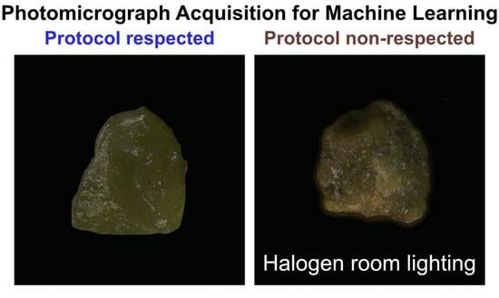
:Identifying minerals is essential for geology, mineral exploration, engineering, and environmental sciences. Recent advances in machine learning have illustrated its potential as a fast, cost-effective, and reliable tool for identifying minerals from photographs or photomicrographs. However, in the recent literature, few studies have been dedicated to image acquisition. Machine learning generally requires reproducible, high-quality data to perform complicated tasks such as mineral identification to avoid common pitfalls. In this paper, we propose a practical image acquisition protocol for optical microscopes. This protocol focuses on ensuring reproducibility and enhancing image quality. To favor reproducibility, we detail dealing with camera errors, using reference color gauges, and establishing experimental parameters such as the external light source and temperature. For image enhancement, we explain the importance of lighting and its impact on machine learning precision, selection of the objective, and white balance calibration. In addition, we trialed the protocol on heavy mineral concentrate from till samples (20 species) with a typical deep learning model and it revealed that minor lighting modification (<5% difference in one channel) significantly increased misclassification rates: kyanite from 6.4% to 24.9% and monazite from 6.5% to 42.9%.
1. Introduction
In many geological studies, knowledge of a sample’s mineralogy is essential throughout a project. During the exploration phase, mineral species and their quantity in glacial sediments provide information on the potential presence of a deposit, such as chalcopyrite in the case of copper deposits or G10 garnets in the case of diamondiferous kimberlites [1,2]. During the exploitation phase of the deposit, mineralogical variation within the deposit can affect performance. For example, phyllosilicates can decrease the efficacy of the crushing process [3]. During the reclamation phase, pollutants may be released depending on the minerals present and the local environmental conditions. In the case of acid mine drainage (AMD), the alteration in sulfides under atmospheric conditions releases pollutants, including arsenic, copper, lead, and zinc [4].
Despite being critical at each phase, mineral identification in sands (especially in heavy mineral concentrates) is an exceptionally time- and resource-consuming process [5]. Identifying millions of submillimeter grains is an arduous and error-prone task. Thus, multiple attempts have been made to pursue automated mineral identification via machine learning [5,6,7,8,9,10]. One promising approach is optical mineral recognition from photomicrographs, as this approach can identify thousands of mineral grains simultaneously, as opposed to current sequential techniques such as the use of a scanning electron microscope (SEM) and identification under an optical microscope by a mineralogist, both of which are costly and long methods. Thanks to the processing speed of this new technique, minerals can be pre-sorted before being sent for further analysis using the two previous methods. It would help to increase analysis capacity.
However, most published AI mineral identification studies rely on their own data sets and use the same photographs for learning and testing the algorithm by randomly dividing the data set items [5,7,11]. The model can therefore be overfit to the specific properties of the images acquired to build the data set and impede the generalization against variability of photographs acquisition. For a more rigorous representation of the algorithm’s true capabilities, tests should be performed on a different set of photographs than that used for learning. In order to improve quality, robustness, and reproducibility, a practical image acquisition protocol is proposed. The theoretical photomicrography acquisition background and acquisition parameters are reviewed, followed by the best practice recommendations. The protocol is applied and tested through a mineral recognition study using machine learning. This protocol will ensure photomicrography quality and reproducibility of mineral identification from an imaging suite.
2. Machine Learning and Optical Identification of Minerals
The number of published papers focused on optical mineral recognition based on machine learning algorithms has increased markedly over the last few years (Figure 1). This heightened interest can be explained by the recent successes of this approach as demonstrated by Maitre et al. [5], Santos et al. [12], and Leroy and Pirard [10], among others. Maitre et al. [5] achieved near 90% grain recognition in a heavy mineral concentrate from till, whereas Santos et al. [12] achieved a success rate of over 80% for determining collotelinite segmentation and coal reflectance. Leroy and Pirard [10] obtained 67% to 90% real-time mineral recognition for particles suspended in water (slurry). Albeit imperfect, these results testify to the enormous potential of machine learning-based optical mineral recognition and quantification.
Mineral photomicrographs acquired with an optical microscope coupled with a machine learning recognition algorithm can provide a fast, low-cost, and reliable means for mineral recognition and quantification. The particles analyzed are larger than those studied via SEM, but they should be sufficient to provide a fast and cost-effective result in most cases. These characteristics will help increase mineral recognition capacity, improve the quantification of mineral abundance, and heighten the reproducibility metrics. The last two benefits are particularly important, as the human eye is not always reliable for quantifying minerals. The inadequate nature of visual identification has been known for decades, and multiple charts have been published for visually estimating mineral percentages to decrease quantification errors [13,14,15]. Visual estimation errors occur mostly because of differences in grain size, shape, and color of the observed grains. Visual estimation bias also comes from the spatial distribution of objects, as observers tend to overestimate object clusters and underestimate distributed objects [16]. A well-calibrated computer-based algorithm does not suffer from these problems and should provide constant results within its bias.
Machine learning mineral recognition, when coupled with optical microscopy, appears to offer an ideal solution. However, this method suffers from inferior attention to the imaging protocol, as highlighted by Pirard and Lebichot [17], and remains inadequately addressed. This lack of a reproducible and accurate image acquisition protocol raises many issues, including segmentation problems and color and textural rendition issues (cleavage, crystallographic form, abrasion, etc.). Changes in lighting and background colors can also alter mineral coloration on the scanned image. Moreover, photographs selected for learning should record identical characteristics as those acquired for mineral identification. Chow and Reyes-Aldasoro [6] applied machine learning mineral recognition using internet-based gemstone photography. They noted that the difference in contrast and saturation caused problems during segmentation, showing the importance of data acquisition for machine learning. As mineral recognition via machine learning is partially based on color, this issue involving contrast and saturation could explain a part of their obtained low accuracy of 46.5% and 69.4% using a random forest and decision tree architecture, respectively, applied to 68 gemstone classes. Jia et al. [9] achieved an excellent average recognition accuracy of 82.23% and 86.54% (ResNET-50 and Vgg16, respectively) for 22 common minerals. They noticed that most misrecognized images originated from inappropriate acquisition conditions that did not show the minerals’ important characteristics. These findings suggest that the refinement of image acquisition protocols can contribute to substantial enhancements in machine learning for mineral identification. Such improvements hold the potential to foster greater robustness in deep learning models, facilitating better generalization across varied acquisition conditions.
Therefore, the photographs used for learning should have identical characteristics (e.g., white balance, color temperature, contrast, saturation) as the photographs of minerals needing to be identified. The qualities of the photographs should be reproducible (precision) and show all key inherent mineral characteristics to ensure proper identification. Moreover, there is growing concern about a reproducibility crisis because of the lack of attention to data acquisition [18,19].
3. Previous Work
The most recent and comprehensive imaging protocol applied to optical mineralogy was performed by Pirard [20]. This protocol was designed specifically for multispectral images, although this technique has much in common with our proposed protocol regarding the acquisition instrument and bias.
Pirard’s protocol has about 350 words in the original article and can be explained as follows:
- Select and keep the same optics and filters throughout the study.
- Set the illumination according to the most reflective mineral to ensure that the images do not saturate.
- Warm up the charge-coupled device (CCD) sensor for up to 90 min.
- Ensure that all images have the same acquisition and processing parameters and avoid file formats with compression.
- Take a black reference image. This image can be obtained by not having any photons hit the camera’s sensor during the acquisition.
- Take a white reference image using a reflectance reference material.
- Acquire a series of images without changing any parameters and apply the image calibration of Equation (1).
Equation (1) was designed for gray-level images, but it can also be applied to color images by correcting the intensity of each channel. This correction allows for altering of the pixel intensity value by considering the thermal noise (or dark current) with the black reference image and the defaults in the optics with the white reference image (e.g., dust and scratches).
This image acquisition protocol is a relevant reference; however, it is relatively simple and short and does not include certain essential parameters to ensure image reproducibility. Indeed, no precaution is given regarding room lighting, and exposure time is not discussed despite its linkage with dark currents and camera noise. Moreover, the warm-up period is arbitrary and does not rely on computation or actual observations.
4. The Theory behind Photomicrographs Acquisition
As photomicrograph acquisition involves many components and related parameters, it is important to study them and describe the relationship between them in order to design an appropriate image acquisition protocol. The three main components are the microscope, camera and image, and the theory associated with each will be presented.
But first, the definitions of the terms used in this study are needed. A camera sensor is composed of physical pixels, which are a group of photodiodes. The number of photodiodes depends on the sensor type. These groups of photodiodes are called camera pixels, and they have a physical size noted . In this paper, we use pixels as the smallest component of an image with coordinates (,. An image thus comprises pixels, and the number of pixels is given by the image size. The pixel value is composed of numbers, often written into brackets, where n is the number of channels of the image’s color space. Channel intensity represents one of the numbers inside the bracket. In a usual 8-bits representation, the intensity for each channel lies between 0 and 255 (). However, many detectors actually have a 12-, 14-, or 16-bit depth per channel. So, if the data can be saved in a RAW format or a variety of proprietary data formats such as the Zeiss CZI, then full bit depth is preserved. In an 8-bit red, green, and blue (RGB) color space, there are three channels: one each for red, green, and blue. The white color is written [255, 255, 255], which is the maximum intensity for the red, green, and blue channels, as white is the sum of all colors. Finally, z-stacking means taking several images along the z-axis to obtain a perfectly focused 3D object over its entire surface.
4.1. Microscope
The microscope is particularly important, as its components play a major role in image acquisition. The important characteristics are its type, objective (or lens), lighting, filters, and software.
4.1.1. Type
Firstly, there are two main types of optical microscope used in geology depending on the sample analysed: grains or thin sections. For thin sections, a petrographic microscope is best because z-stacking will not be an issue. Manufacturers offer a wide range of petrographic microscopes and tools that can be added for more specific applications. If many thin sections are to be analyzed, a slide scanner can be used. An on-axis zoom microscope is ideal for grains if the studied material is not too fine. The latter’s advantage is that it gives a higher depth of field and a larger field of view than the petrographic microscope. This advantage markedly reduces the acquisition time for grain analysis.
Essential options for both microscopes include a computer-controlled motorized stage for seamless sample acquisition without continuous user intervention. For thin sections, an x-and-y-axis-controlled stage is generally adequate, but non-flat-surface sections may require z-stacking for precise mosaic photomicrography. Grain photomicrography necessitates a z-controlled axis. If a motorized stage is not available, photomicrographs can be acquired, stitched, and Z-stacked manually. However, it would take an enormous amount of time. Additional beneficial features comprise a computer-controlled rotating polarizer for capturing polarized images at various angles without grain movement [21], enabling simultaneous image capture without manual intervention. The optimal configuration involves a fully computer-controlled microscope for this innovative technique.
4.1.2. Objective, Lighting, and Filters
Secondly, the objective, lighting, and filters must be taken together. A changeset in one of them influences the others. Their relations are mathematically described through the existence of parameters and equations linking them. These equations use a monochromatic light source instead of a polychromatic one but are still widely used for estimating microscope parameters. The parameters related to the objective are the numerical aperture (), magnification (), and depth of field (). The parameter related to the lighting is its wavelength (). The filters are not properly defined in the following equations but play an important role as they can modify the lighting wavelength, polarization, or intensity.
To compute the minimum spatial resolution () possible for an optical microscope, the Rayleigh criterion is used and can be explained as follows (2). The microscope’s minimal resolution is related to the diffraction itself, and the image of the smallest light point through a microscope will be an airy disk. If two points are side by side, it is possible to distinguish one from another only if the distance between each other is superior or equal to their airy disk radius () [22].
Nevertheless, the optical microscope in this study is paired with a camera that has its own spatial resolution (). This resolution limit is the camera pixel size (. Thus, it is possible to compute the camera spatial resolution mounted on the microscope by multiplying with the magnification of all the microscope optical elements. In most cases, they should have the objective and camera adapter magnification, respectively, and (Equation (3)).
The camera’s spatial resolution needs to be better than that of the microscope since the microscope sets the highest-resolution limit. In the case of 3D object acquisition of mineral grains, and because most microscopes have a short depth of field, multiple stacked images are needed (z-stacking). Therefore, to calculate the total microscope depth of field, we must sum the wave and geometrical depth of field (4).
where is the depth of field, is the wavelength of the light source, representing the refraction index of the medium (air in our case), is the objective numerical aperture (given by the manufacturer), is the objective magnification, and is the camera pixel size (given by the manufacturer).
Equation (4) is from Inoué and Spring [23] and is slightly modified to match our study’s needs. The geometrical depth of field (the last term in the equation) is multiplied by , which is the physical size of a camera pixel. Normally, this parameter is called and represents the smallest distance resolved by a detector placed on the image plane of the microscope [22]. The assumption in this equation is that the camera cannot resolve an object smaller than its pixel size.
By dividing the height of the larger object () by the total depth of field, we can determine the necessary number of z-frames () (Equation (5)). Thin sections may require z-stacking because of their uneven thickness, often . For grains, the size of the coarsest grains can be obtained using sieves or laser diffraction. Adding one frame is needed when the depth of field is larger than the object’s maximum height.
For grain analyses, a low-NA objective is ideal as it requires the fewest z-frames. Therefore, the spatial resolution of the microscope will increase, and the grain size will need to be coarser to maintain an acceptable number of pixels per grain. For thin section analysis, however, it is possible to choose a high-NA objective for more precise measurements, as z-stacking is unnecessary. However, a smaller camera resolution is needed to match the reduced microscope spatial resolution, leading to a greater demand for storage capacity for the same study area (Equation (7)).
It is imperative to choose the objective carefully. In microscopy, numerical aperture is often used to describe the light accumulation and resolution capacity of the objective as opposed to the angular aperture (, used in photography). However, these values are linked by Equation (6) with representing the refraction index ( in air). As numerical aperture and angular aperture are linked proportionally, only the numerical aperture is discussed.
Numerical aperture is proportional to the microscope’s spatial resolution, as a higher numerical aperture results in a higher resolution (Equation (2)). However, the numerical aperture is also directly related to the depth of field, a critical parameter for z-stacking and, thus, grain photomicrography. The depth of field decreases as numerical aperture increases (Equation (4)); therefore, the objective must be carefully chosen based on its numerical aperture. The numerical aperture, via the presented equations, must match the camera’s resolution, the size of the studied object, and the desired depth of field.
4.1.3. Microscope Hardware
Finally, the microscope software plays an important role in limiting the choice of image file extension, color space and routine, or advanced parameterization options. The first two of these issues will be addressed in the image sections, while the last will be covered in the discussion.
4.2. Camera
The central piece of equipment for image acquisition is the camera. Even if the camera is a component of the microscope, it needs its own section as its characteristics greatly influence the image quality and reproducibility, such as the depth of field seen in the prior section (4). The important camera characteristics are its type and manufacture quality, noise, and warm-up period.
Two types of cameras are currently used in optical microscopy: charge-coupled device (CCD) and complementary metal–oxide–semiconductor (CMOS). Camera selection depends on the study’s objectives. A CMOS camera has a good image quality and allows for real-time data acquisition with its high frame rate [10]. Using an intensified CMOS camera allows for measurements at very low illumination with a moderate signal-to-noise ratio (SNR). SNR is the ratio between the mean signal value and its standard deviation. However, using an intensified CMOS camera leads to a lower resolution. CCD cameras have a high signal-to-noise ratio and a greater image uniformity than CMOS. This allows for them to have a better image quality than CMOS; thus, CCD cameras should be used for precision measurements [24]. However, recent articles indicate the quality difference between CMOS and CCD in regard to high-quality imaging is narrowing [25,26].
Cameras are subject to three main noise sources: thermal noise, camera readout noise, and shot noise. Thermal noise, or dark noise, stems from the charge induced by the thermal fluctuation of the camera components. This noise depends on the camera itself, but external factors are also involved. Thermal noise is proportional to exposure time and temperature, which limits the quality of the longest exposures. This noise can be markedly reduced by cooling the camera. The camera readout noise is produced through its own architecture and components; this noise is inherent to each camera and does not depend on external factors. Finally, shot noise expresses the probability that a random photon hits the camera’s photosensitive sensor. Thus, for each acquisition with the same lighting, exposure time, and camera, different amounts of photons will hit the sensor. Moreover, the resulting images differ slightly from each other [27].
Lastly, cameras are subject to thermal noise and their use generates heat, as is the case with computer processors, so they require a certain warm-up period to reach a stable temperature and error [20]. This parameter will be decisive for image acquisition, as it maximizes noise but ensures reproducibility by having the same amount of noise for each image.
4.3. Image
The final stage of acquisition is the image itself, but many parameters are linked to it. Important characteristics of the image are the exposure and computer parameters: image format, color space, and volume.
Exposure defines the time during which the camera accumulates light on its photodiodes. Exposure is therefore closely linked to illumination intensity, which depends on the room lighting and microscope illumination voltage, as well as the presence of filters. This parameter is crucial, as it can saturate mineral images if the time is too long and renders the image completely black if it is too short.
Regarding the computer parameters, all are linked with each other. The first one to be described is the image format. Depending on the microscope software, there is a limited choice in image format. The most common image formats are JPEG, PNG, GIF, TIFF, and BMP. JPEG is a compressed format with a loss of information, but it has great portability. PNG files are compressed without information loss and also have great portability. GIF format can undergo greater compression than PNG without any information loss; however, it has a restricted number of color shades. TIFF is a very versatile format and accepts all color formats and color spaces. It can also store raw data from the photographic sensor (often called “RAW”) and multiple images per file. BMP files have very good portability and are easy to use. BMP is an uncompressed file format; however, its size can be reduced by using an algorithm like ZIP.
Another important parameter is the color space, which defines how colors are represented. A color space is an -dimensional space in which each color is represented by a vector with components equal to the dimensions of the color space [28]. The most common color spaces are RGB and CMYK; they have 3 and 4 dimensions, respectively. Each existing color space has its particularities and does not represent the entire color gamut. Depending on the software, it may be possible to choose a color space such as AdobeRGB, sRGB, or ProPhoto RGB. The ideal would be to choose the color space having the largest color range. However, to represent all color possibilities, the bit depth () must be higher because more information is needed. Thus, the image volume will increase (Equation (7)):
where is the image volume in octets, is the image height in pixels, is the image length in pixels, and is the bit number per pixel or bit depth. and are given in the image resolution. For example, an image with a resolution of 1920 2560 means that and pixels each. The should be specified in the microscope software parameters; currently, it is generally 24-, or 8-bits per color channel. Thus, the volume of this image would be approximately equal to 118 MB.
The photomicrography color space must also match the data sheet provided by the reference color gauge manufacturer to compare the acquisition with its laboratory value. These choices depend on the computer, its storage capacity, and the microscope settings (see the following section). It is possible to compute in advance the image volume for equipment selection (7).
Nevertheless, the image acquisition of an entire thin section or grain mount requires dealing with composite images, such as those generated via z-stacking. A major issue is the storage capacity and the need to have a sufficiently large hard drive (the size depends on how the software combines the images). The following equation assumes that the microscope software starts processing the composite image only after all the temporary images are taken (Equation (8)). Therefore, all the acquired photomicrographs must be saved temporarily on the computer.
where is the total volume of the temporary images in octets, is the length in image number of the acquired zone, is the height in image number of the acquired zone, and is the image number stacked vertically. An example of the total temporary volume generated by the acquisition of one grain slide is 764.64 GB: each image weighs 118 MB and the mosaic image is composed of 12 × 27 photomicrographs with a stack of 20 photomicrographs along the z-axis.
5. Protocol Design Recommendation
As highlighted by the previous sections, each one of the main photomicrograph acquisition components is strongly linked to the other by its parameters. It also appears that photomicrograph acquisition is sensitive to external factors such as room temperature and lighting. Moreover, it is important to design the acquisition according to the object of study. The figure below shows the relation between the acquisition components and related parameters (Figure 2).
The acquisition of a photomicrograph can be divided into three main parts: (1) The purpose of the study, in which the object of the study is defined and the influence of external factors is discussed; (2) The parameter settings, in which the parameters are tested in order to find the best compromise; (3) The acquisition routine, in which the application of the parameters and the analysis of reproducibility are discussed.
5.1. Study Purpose
First, it is important to define the type of sample and what we are looking for. Depending on the answer, it will be possible to define the resolution required for the study, and to examine the most reflective or translucent mineral in the sample data set. External factors remain the same and they will be considered in the following sections.
5.2. Parameters Settings
5.2.1. Lighting and Exposure
The lighting must be the same at each acquisition to ensure reproducibility by limiting illumination variability. The position of the light source and its intensity must therefore be set precisely and kept constant. If the light source is filtered, the same filter must be applied for the entire study [20]. Note that the stronger the light intensity, the shorter the exposure time, which decreases thermal noise and shortens the acquisition time. The best way to calibrate light and exposure time is to set the light intensity at its maximum and increase exposure time until the most reflective and the most translucent mineral or color gauge saturates. The optimal exposure time will be just before saturation.
5.2.2. Objective Choice
The numerical aperture is the most important parameter in the depth of field equation and microscope spatial resolution. The choice of the other parameters, such as the camera resolution and the frame number for the z-stacking (Equations (2)–(5)), depends on these two computations. Also, the best way to choose your objective is by using its numerical aperture and magnification. This makes it possible to model depth of field as a function of the numerical aperture (Equation (4)).
5.2.3. Room Lighting and Noise
The most critical parameter for image acquisition is light. Room lighting (e.g., artificial lights, sun exposure) influences image acquisition and, more importantly, reproducibility. The first step is to remove the microscope from ambient light. There are two means to do this: by locating the microscope in a room where outside light sources are blocked or by building an enclosure or shroud around the microscope (Figure 6). According to the authors’ experience, an enclosure is preferred because:
- No external light affects image acquisition.
- Camera tests are much easier to perform.
- Dust and unwanted particles are kept away from the microscope and samples.
However, enclosing the setup poses a drawback as it traps warm air generated by the light source and electronics. Camera noise is influenced by temperature and exposure time, and introducing a cooling system, such as a Peltier cooler or fans, can mitigate this issue. Nevertheless, vibrations from these components may arise. Alternatively, a ventilation system with openings at the top and bottom of the enclosure can be employed. Air convection may suffice for camera cooling while maintaining a stable temperature. Nonetheless, the ventilation design must effectively prevent external light pollution.
Cameras experience thermal noise and necessitate a warm-up period for temperature stabilization. Pirard [20], in his image acquisition protocol for optical microscopes, recommended letting the camera warm up for about 90 min. Although this recommendation can be valid, it is advisable to determine a specific warm-up period for the camera in use. The simplest way to do it is as follows:
- Verify that the microscope camera is at room temperature.
- Ensure that no stray light strikes the camera sensor (use an enclosure or other means to ensure complete darkness).
- Turn on the microscope, computer, software, and NO lighting.
- Take pictures every 15 min for at least 3 h.
- Use any coding language to extract the pixel intensity values for each channel from the image. This must be performed for each image.
- Plot a graph of the time using the equation (9, versus the mean intensity per image for each channel) (see Figure 7).
- where is the time, is the frame number, and is the frame rate.
- Analyze the graph. Ideally, the graph will show increasing mean pixel intensity value for each channel up to a plateau. From the moment the curve stabilizes around a particular value, the camera has warmed and the error is constant.
- Identify the stabilization point marking the time needed to warm up the camera before image acquisition.
- This procedure will ensure the reproducibility of the acquisition. However, the dark current error during the acquisition will be at its maximum. In most cases, this noise will be minimal to negligible.
5.3. Acquisition Routine
5.3.1. Sample Preparation
We test two grain-mounting techniques (permanent and temporary), the choice of mounting depending on the used ground-truth acquisition technique. Ground-truthing in machine learning is defined as using an independent and accurate method to verify the algorithm prediction. Here, we obtained our ground truths either by SEM cartography or by visual sorting (handpicking) of the minerals by a qualified mineralogist.
The permanent mounting technique must be vacuum proof, as the ground truth is acquired by SEM X-ray fluorescence. The grains are glued onto a 1 mm thick glass slide using epoxy. A permanent slide can be produced in three steps:
- Place a glass slide on a perfectly horizontal plate covered with aluminum foil. Tape the edges of the glass slide to secure it to the foil (Figure 3A). This step prevents the epoxy from flowing underneath the glass slide and facilitates removing the glass slide after the curing.
- Apply epoxy to the glass slide (a 5 µm thick layer) using a micrometer-adjustable film applicator (Figure 3B), powder the grain, and wait until the permanent slide is cured. Powdering should be performed to minimize grain overlap and evenly distribute grains. Curing time depends on the epoxy, and we suggest using transparent epoxy with a high viscosity to prevent the grains from sinking too deeply.
- Remove the adhesive tape and glass slide from the aluminum foil (Figure 3C).
Temporary mounting consists of “sticking” grains with ethanol on a 1 mm thick glass slide as follows:
- Put a few drops of ethanol on the glass slide, just enough to have a thin film of ethanol that does not flow outside the slide (Figure 4A).
- Powder the grains uniformly so that the grains are evenly spaced on the slide (Figure 4B).
- Wait approximately five minutes for the ethanol to evaporate (leaving a dry slide). The slide is ready for photomicrography.
- After photomicrography, grains can be easily scraped from the slide with a laboratory spatula and recovered for another use (Figure 4C).
No additional sample preparation is needed for thin sections, except dust particles and potential oxidation of certain minerals like sulphides, which should be cleaned or repolished.
5.3.2. Photomicrography
We acquired a color gauge from Image Science Associates (ISA) for this study. We selected the Pico model for its size (9.5 mm large, 11 mm long, and 1.5 mm thick, the smallest size available). Each colored square measures 1.58 mm on a side (Figure 5B). The color gauge is provided with its color value datasheet in multiple color spaces: CIELAB, Adobe RGB, sRGB, ProPhoto RGB, and ECI-RGB v2 (Figure 5A).
A white balance must be performed on an 18% gray card before each acquisition and at each lighting change to ensure that the acquisition method remains constant and reproducible (Figure 5). A sample holder will help automate image acquisition; it ensures a regular acquisition with fixed positions for the color gauge and, in some cases, the most reflective mineral, the thin section, and the grid (Figure 6B). This grid can be added to the sample holder to ensure that the microscope optics do not distort the objects on the image [29].
We developed a routine for color gauge analysis to understand color acquisition as a function of camera and lighting. We aimed to compare the mean value of the color gauge photomicrography for each acquisition with its theoretical value. The routine steps are:
- Set up the entire acquisition to respect all protocol recommendations and steps, such as microscope enclosure, calculated camera warm-up period, and white balance calibration.
- Acquire a series of images of the color gauge at various times and moments of the day to ensure that the color variation is not related to the ambient light change.
- Segment the color gauge from the sample holder for the entire picture series to obtain only the region with the given color(s). For example, if the color gauge comprises several patches having different color codes, subdivide the image to achieve one image per given color code.
- For each cropped image, compute the mean pixel intensity value of the acquisition () and the standard deviation () for each channel over the entire series.
- Extract theoretical pixel intensity values for a given zone () for the color gauge from the manufacturer’s data sheet for the same color space.
- Compute the difference () between the theoretical pixel intensity values of the color gauge () and the mean pixel intensity values of the acquisition () using Equation (10).
Plot versus to compare the acquisitions. For each point, use for the error bars. This diagram will present pixel intensity as a function of its theoretical intensity for each channel (Figure 8).
This graph answers two critical questions: (1) Is camera color acquisition dependent on pixel intensity? (2) Is the acquisition constant for each pixel intensity when using ?
6. An Application of the Protocol
In our previous work [5,30], our team worked on mineral grain recognition. Like other studies [5,7,11], we used a data set built from one acquisition session for both the training and the testing. Testing in such a manner does not ensure generalization across acquisition variability and may also impede the robustness of the model. To ensure fair assessment, it would be better to test on a new acquisition. For that, our protocol may prove to be quite useful since its aim is to provide a framework for repeatable and good quality image acquisition. As a trial of this protocol, we applied it to a mineralogical recognition using a heavy mineral concentrate from till sediments. We purposely made several acquisitions to create the training and testing data sets. This section presents the details of the application of our protocol for this example machine learning task.
6.1. Microscope Enclosure and Sample Holder
We built an aluminum box enclosure to prevent the impact of the room lighting (60.5 cm large × 117.5 cm long × 76.5 cm high). Although microscope enclosure limits its access, it is mandatory to limit external light source. Alternatively, the microscope can be used in a dark room with all external lights off. (Figure 6A). The sample holder was of poly(methyl methacrylate), known commercially as plexiglass—with a fixed position for the color gauge and two mineral mounts (glass section), each 2.5 cm wide, 7.5 cm long, and 0.1 cm thick (Figure 6B).
6.2. Acquisition Settings
The camera and computer settings are given in Table 1. We used an annular LED light that was added to a BX53M optical microscope equipped with a SC50 camera, both from Olympus (Shinjuku, Tokyo, Japan). The light holder made for the study ensured a fixed position.
6.3. Machine Learning Requirements and Sample Preparation
During the training, validation, and testing, the machine learning algorithm requires a photomicrograph or photomicrographs and the corresponding label for each grain. The label, in our case, is the grain’s mineralogy. This label is known through ground-truthing and depending on the form of ground-truthing, some limitations exist. The mineral species grain population must also be approximately balanced during this process as unbalanced classes lower algorithm performance.
The permanent mounting can handle several types of mineralogy on the same glass slide because of the fixed position of grains and SEM cartography where the coordinates of each grain and its mineralogy are recorded. This is the approach we relied on in our previous work [5,30]. However, this method involves higher risk. If the sample is poorly prepared, it is impossible to recover it. For the temporary mounting, as the mineral grain composition is known before the acquisition because of sorting by a mineralogist, it is easier to adjust grain quantity and balance the different mineralogy. The easiest way to acquire the data set is to take one mineral per image; this way, the image will work as the label. Each grain present on the photomicrograph is from the chosen mineralogy. If several minerals are mixed on the same photomicrograph, a map with the position and mineralogy of each grain is needed. A drawback of this technique is that the temporary mounting is highly dependent on the quality of the visual sorting phase.
Once the algorithm has learned from the training microphotographs, none of the previously announced limitations remain active. Both techniques can handle several minerals per glass section, and an algorithm that has learned with the permanent mounting would be able to identify grains on a temporary mounting and vice versa. The only requirement is that the optical properties of the grains are conserved for both techniques; thus, neither the epoxy nor any alcohol must cover the grain. Table 2 describes the appropriate lighting for each mounting technique.
The grain mineral species collection for this study comprised 20 mineral species in the learning data set, with two testing groups containing a minimum of 50 and 20 grains per species. Some samples were obtained from Maitre et al.’s [5] analysis. Temporary mounting was employed for image acquisition, enabling testing of various setups without fixing grains and minimizing the risk of mounting failure.
6.4. Machine Learning Model
To demonstrate the added value of our methodology, we trained a convolutional neural network (CNN) model for approximately 7.5 h (27,212.48 s) on a data set containing the photomicrographs of the grain mineral species collection. The CNN is a standard architecture of 8 convolution layers with filter size [32, 32, 64, 64, 128, 128, 256, 256] and ReLU activation. The kernels are in decreasing size from (7, 7) for the first two layers, then (5, 5) for the next two, and (3,3) until the end. All conv layers have stride (2, 2) to down sample, batch normalization to stabilize the training, and pair layers have a drop out of 20%. The CNN ends up with a classic double layer of dense units, respectively, 256 and 128. Then, after a final dropout, there is the last layer for classification (20 units). Overall, this is a classic CNN for classification that has 1 418 548 trainable parameters.
The learning process comprised three steps: (1) training, (2) validation, and (3) testing. For each step, a related data set was dedicated with a known number of images per mineral (Table 3). The photomicrographs used for the CNN training followed our protocol (Table 2). The accuracy of the trained model was 88.7%, the balanced accuracy was 87.7%, and the Cohen–Kappa score was 88.1%. In this paper, we do not focus on the quality of the classification results, only their reproducibility. For SoTA models, we instead refer the reader to the literature on deep learning [31].
7. Protocol Application Results
7.1. Warm-Up Period
We established the warm-up period (Figure 7) by capturing a black image every 15 min for 6 h (360 min). The acquisition resolution, exposure time, and all settings used for this test were identical to those of the grain image acquisitions except the enclosure presence (Table 1). The black image pixel intensity for the red, green, and blue channels were extracted using the Python imaging library (PIL). In order to understand the role of temperature, a thermocouple was installed on the top of the camera. The measure rate was one per minute.
The room temperature was measured for 179 h (n = 10741) at different times and on different days, giving an average temperature of 22.13 °C ± 0.23. The starting temperature of the warm-up period test is sometimes around 23 °C, as the microscope must be switched on before the computer, and the temperature starts to rise at the same time. The warm-up period diagram clearly shows that the temperature rises when the camera is used for an extended period. Diagrams A and B show the impact of the microscope enclosure on temperature. The first and second tests show an increase in temperature to 26.22 °C and 24.64 °C at the end of the test, respectively. This means that the presence of the enclosure generates an overheating of 1.58 °C (Figure 7).
However, despite the temperature difference, the error for each channel is very similar for both tests. For diagram A, the mean values of the R, G and B channels for the whole test are: 0.665 ± 0.501, 0.665 ± 0.501 and 0.301 ± 0.470. And for diagram B, the mean values of the R, G and B channels for the whole test are: 0.660 ± 0.501, 0.660 ± 0.501 and 0.291 ± 0.465. It appears that the first 150 min are more stable for the blue channel in both tests, but the difference is not significant, as the error is around 0.3 on a scale of 255 (Figure 7).
Further tests were carried out with a higher exposure time (32.01 ms) and a smaller enclosure (42 cm large × 47 cm long × 67 cm high), with a total of 8 tests. Except for the higher temperature (27.82 °C) with the smaller enclosure, the error is still very similar between these tests. The warm-up period is set at 150 min to ensure that the temperature has reached a plateau.
7.2. Color Gauge Information and Analysis
7.2.1. Reproducibility Analysis
The theoretical intensity for each channel was calculated under the D50 illuminant. The D50 illuminant represents daylight and is described by its spectral power distribution (illuminants are defined by the Commission Internationale de l’Éclairage (CIE)). The light source of our study differed from that used to calibrate the color gauge. Hence, we used the theoretical pixel intensity as a reference, and an unknown portion of the difference (∆) stemmed from the inequality of the lighting sources. The color gauge comprised 30 squares, each having a red, green, and blue intensity value (Figure 5A).
For each color present on the color gauge, we used Python 3 to compute and extract the mean pixel intensity of the acquisition (), the mean pixel intensity standard deviation (), the theoretical pixel intensity (), and .
For presentation purposes, the reference colors were divided into two for plotting pixel intensity as a function of its theoretical intensity (Figure 8). The grayscale squares (Figure 8A) range from white to black. Their particularity is to have very similar red, green, and blue channel values; for example, the gray square (1,1) intensity value of each channel according to the manufacturer is [203,204,203] for the red, green, and blue channels, respectively (Figure 5A). The second group, the color squares, is located on the border of the color gauge (Figure 8B). Their particularity is to have a significant value difference for at least two channels.
The grayscale and color squares behaved differently (Figure 8). The grayscale squares had a negative for values between 23 and 118 and a positive for values between 148 and 242. Therefore, relative to the theoretical intensity, the low-intensity values were overestimated, and the high-intensity values were underestimated. The grayscale range of the acquisition was smaller. For the color squares, the values were positive and close to 0. The exception was for seven color squares where the blue channel had a negative value close to 0 (−2.1% maximum). Overall, the color squares intensity was well estimated, as most values were between 0% and 5.9%. However, the color squares presented a smaller range of values (53–227) and more extreme intensity values were missing, unlike the grayscale group (23–242). Overall, this independent demonstration of machine learning shows that the color gauge images have a very similar pattern and that their acquisition was reproducible.
7.2.2. Parameters Impact
To understand and demonstrate the impact of acquisition parameters, 8 tests were carried out. During these tests, an epidote grain (Figure 9) was acquired with the color gauge (Figure 5). Only the red, green, and blue squares were analyzed and are presented in the graph below (Figure 10, Figure 11 and Figure 12). The acquisition parameters are the same as those shown in Table 1 and the whole protocol was respected, with specified variation.
The detailed test parameters are described in the Table 4. Test 1 aims to measure the impact of the warm-up period, tests 2 and 3 simulate the impact of room lighting after white balance calibration, tests 4 and 5 focus on the importance of exposure time, tests 6 and 8 on the role of light intensity, and finally test 7 will serve as a comparison as it fully complies with the present protocol. Test 8 was an attempt to reproduce the images of test 7 with a medium light intensity, and the exposure time was modified accordingly.
Tests 2 and 3 explore the impact of changes in room lighting after white balance calibration. And despite the visible difference on the epidote image (Figure 9), the graph above shows us that these variations remain below the 5% limit of difference with the reference image. Test 3 is more anomalous than test 2, with a higher average red intensity value for each square. In addition, each high intensity value representing the main color of the square shows a significant difference. Test 2 remains close to the y = x line, except for the red channel of the red square, where the difference is greater. The average blue intensity value for test 2 is lower for each square (Figure 10). Finally, these tests show differences despite all respecting Pirard’s recommendation (Table 4).
Tests 4 and 5 show the impact of changing exposure time without changing light intensity. Test 4, with its longer exposure time (8.991 ms), shows a higher average intensity value for each channel. Test 5, with a shorter exposure time (2.999 ms), has a lower average intensity value for each channel. The graphs also show that the higher the average intensity value, the greater the difference caused by changes in exposure time. For example, the reference blue intensity values are 28.24, 49.14, and 83.45 and the difference increases for both tests by 10.11, 15.34, and 19.94 for test 4 and by 12.40, 18.73, and 20.37 for test 5 (Figure 11).
Test 1, which is the replication of the protocol without the warm-up period, is close to the y = x line, except for the blue channel of the blue square, where the difference reaches 3.09%. Test 6, which shows a decrease in light intensity, behaves similarly to the exposure time. The difference is greater with a higher intensity value. Finally, test 8, which attempts to reproduce the image of test 7 with lower light intensity and higher exposure time, shows similar behaviour to tests 4, 5, and 6, consistent with the changes made to the acquisition parameters (Figure 12).
7.3. Impact of Warm-Up Period and Room Lighting on Classification Results
Two test groups were acquired five times at different moments and on different days, strictly adhering to the image acquisition protocol (AL series, Figure 13A–C). The test groups were also acquired for a warm-up period of 0 (labelled WP-0) and 100 min (labelled WP-100), rather than 150 min, as determined earlier (Figure 13D). To evaluate the reproducibility of our mineral classifications with modified acquisition parameters, we then modified the AL series to simulate a change in ambient light: a halogen light source with a color temperature of 4500 K (labelled 45K; Figure 13E) and overcast daylight with a color temperature of 7500 K (labelled 75K; Figure 13F).
For the nine acquisitions of the AL–WP0–WP100 series (Figure 14), the number of detected grains varied from 482 to 516 (mean: 501, SD 11.6). For the 45K and 75K series, the number of detected grained varied from 465 to 492 (mean: 477, SD 11.4) for 45K and from 474 to 497 (mean: 485, SD 8.42) for 75K. The difference in the number of identified grains can be explained by 1) the presence of dust, which is segmented as a proper grain; 2) segmentation artifacts because of grain reflection and stitching errors; and 3) grains segmented more than once because of their presence at the edges of several images.
We observed no significant difference between the acquisitions that strictly followed the protocol and those with a warm-up period less than 150 min (Figure 14A,C). The proportion of detected minerals was constant, except for diopside and rutile, for which the results appear less precise, evidenced by the relatively high standard deviation (Figure 14B,D). This lower precision is related to the low number of images in the learning data set for rutile (Table 3) and the high similarity of diopside with amphibole.
Using the same photomicrographs with a change in the ambient light (Figure 15A,C), the grain proportion per mineral varied markedly relative to the ideal acquisition (Figure 13A). The mean relative difference of both the 45K and 75K series (Figure 15B,D) was also higher than that for the AL series (Figure 14B). However, the repeatability of the classification appeared stable using this changeset simulation, although some minerals were overrepresented: monazite (>40%) for the 45K series and kyanite (>25%) for the 75K series. This overestimation explains why the relative standard deviation of the other minerals was high, given their small proportion.
The misclassification observed when simulating changes in lighting conditions during acquisition could be due to a strong variation in the intensity of the red, green, and blue channels. However, by examining the intensity of each channel for all images in Figure 13, the maximum observed difference is between the epidote A and E. The difference is 10.47 or 4.12% for the green channel. Moreover, these differences are in accordance with the differences obtained using real LED and halogen lighting (tests 1, 2, 3, and 7). The standard deviation within each image is high due to the presence of relief at the grain surface (Table 5).
Our classification showed great reproducibility, as the grain proportions per mineral within a given series were very similar. Nonetheless, the low number of grains (approximately 20 per mineral) heightened the mean relative difference between each series and the minerals. These tests also highlight the sensitivity of machine learning to change of less than 5% in image intensity.
8. Discussion
This paper aimed to describe and demonstrate a protocol to ensure the reproducibility and quality of image acquisition, making it suitable for machine learning applications in mineralogy.
8.1. Grain-Mounting Technique
We presented two complementary techniques for mounting grains on a slide. The critical element for mounting is that the adhesive medium does not alter the optical properties of the grain; thus, a variety of media are possible depending on availability, regardless of the step in this machine learning-adapted protocol. The aim of the mounting is to acquire photomicrographs with all the possibilities offered by a microscope. Selecting the appropriate adhesive also depends on the lighting used. A future study should assess the advantages of epoxy staining; such an approach could significantly improve the grain segmentation for transparent minerals in grain mounts, such as quartz, that have a color and transparency close to that of epoxy.
8.2. Cameras and Microscopes
We faced a disk space limitation due to the grain topography requiring a high number of z-images, but it was set at 20, as this was the maximum possible. Decreasing the objective magnification could have been a solution; however, the 2.5 objective was subject to vignetting. This explained our recommendation to use an on-axis microscope for grain imaging as the depth of field is higher and would have decreased the number of z-images necessary.
Our protocol also illustrates the need for more appropriate microscope software. Some commercial software does not allow the user to adjust the acquisition parameters. For example, it is often impossible to adjust the stitching margins, and only the completed stitched photomicrograph is available, not individual photomicrographs. With Python and ArcGIS, routines are readily available and are used extensively by industry, and such an addition to optical microscope acquisition software would be beneficial. A huge step forward for numerical petrography would be to develop more open software linked to the microscope equipment. A second would be to make all microscope parameters computer controlled, including lighting type and its focusing and its intensity, polarization filters and their orientation, and the objective and its focus. As Fueten [21] noted concerning computer-controlled stages and rotating polarizing filters, these improvements will significantly expand the potential uses of the petrographic microscope in geological image-processing applications.
8.3. Computer Settings
An issue related to the black-box software is the pixel size of the images at the end of the process. It is possible to use the scale bar given by the software and microscope manufacturer; however, it is nearly impossible to know the detailed computation and steps behind this process. Thus, this information related to pixel size is not reliable when developing a new method. In our study, the link between the camera pixel size and image pixel size was not detailed, preventing the straightforward definition of the photomicrograph pixel size. Therefore, the only reliable method to determine photomicrograph pixel size is to measure different parts of the color gauge in pixels at each acquisition. From this, a ratio (and its standard deviation) can be computed for the length in pixels and the metric length. It would be possible to study the evolution of pixel size among acquisitions, as this parameter may vary. However, studies should investigate the data flow and transformation from camera to software, as it might be possible to shortcut the data treatment for real-time data acquisition.
8.4. Exposure and White Balance Calibration
For this study, we performed white balance calibration using an 18% gray card, as recommended by professional photographers. However, it would be relevant to study the effect of the color chosen for white balance calibration on image quality. Moreover, all photomicrographs were acquired with maximum light intensity and minimum exposure time to minimize the dark current error. However, the warm-up computation and classification results showed that this error had a negligible effect on annular light photomicrographs. Therefore, studying the difference between photomicrographs of minerals acquired with the shortest exposition time and maximum light intensity and those captured using a longer exposition time and a medium light intensity would be relevant. The longest exposition time possible would not be relevant, as the dark current error would be too high in such a scenario.
8.5. Color Gauge Analysis
The color gauge role in this study determined whether the camera and its color representation depended on pixel intensity and whether the acquisition was constant for each pixel intensity. However, the color gauge can also be used for color correction and, if a reference color gauge is chosen, it would be possible to have the same computer representation of color independent of the microscope and camera type. This step would be critical for implementing this protocol. However, the color gauge used in this study is not suitable for transmitted light images as it is opaque. Another drawback is the texture on the surface of the color square that generates reflection and shadows, which might partly explain the standard deviation of each color channel. Thus, the best solution would be a translucid flat color gauge.
8.6. Classification Results
Our classification showed great reproducibility between acquisitions and highlighted the importance of an image acquisition protocol. By altering the ambient light, we noted that the algorithm’s classification changed markedly, but the channel intensity did not, with a variation of less than 5%, confirming the sensitivity of the method and the importance of controlling each acquisition parameter. The only means of achieving this control is to follow a strict and complete image acquisition protocol. The dark current error, however, was not sufficiently large for this type of photomicrograph (approximately 0.7 on a scale of 0 to 255 for the red and green channel and 0.3 for the blue channel) to affect the classification results. However, photomicrographs requiring a more extended exposition time may produce more significant classification errors.
9. Conclusions
The protocol presented in this paper can be summarized as follows:
- Mount the grains or rock without alteration in the useful optical properties for the study.
- Choose between a petrographic microscope for thin section and an on-axis zoom microscope for grains, ideally.
- Compute the ideal image size and your storage capacity and act accordingly.
- Microscope noise sources:
- Create an enclosure for the microscope, as it prevents external light and dust pollution.
- Compute two or three times the warm-up period at different times of the day, if your laboratory is air-conditioned and the exposure time is small it should not have any impact on the image quality. If the error is high or not stabilizing, measure the camera temperature or cool down the camera.
- Use a color gauge to calibrate and study your acquisition parameters.
- Choose the objective based on the spatial resolution required for your study, the camera resolution should be superior to that of the microscope. And use the same equipment for the whole study.
- Adequate documentation on photomicrograph acquisition should be included with images.
This image acquisition protocol addressed the mounting of the grains, the settings and parameters of the computer and microscope, the use of a color gauge, and the sources of noise and errors in the image acquisition using an optical microscope while also specifying its physical observation limits. The links between each parameter are described and the beginnings of solutions are given. Our protocol also ensured the reproducibility of images and provided a critical assessment of acquisition through analysis of the color representation of the camera and its warm-up period. The standardization of the acquisition data permitted us to detail the sensitivity of automated learning to changes in the training data. Our research underscores the importance of implementing a rigorous image acquisition protocol to achieve consistent and replicable classification results. The meticulous steps outlined in our study are designed to guarantee the method’s precision across diverse materials and objects of study.
Author Contributions
Conceptualization, A.L.B. and L.P.B.; methodology, A.L.B. and L.P.B.; validation, A.L.B., L.P.B., J.M. and K.B.; writing—original draft preparation, A.L.B.; writing—review and editing, A.L.B., L.P.B., J.M. and K.B.; Supervision, L.P.B. and J.M.; Project Administration, L.P.B.; Funding Acquisition, L.P.B. All authors have read and agreed to the published version of the manuscript.
Funding
This study was funded by a Fonds de Recherche du Québec - Nature et Technologies (FRQ-NT) grant to L.P.B. Programme de recherche en partenariat sur le développement durable du secteur minier-II, grant number: 2020-MN-283346, with contributions from IOS Servives Géoscientifiques Inc.
Data Availability Statement
The data presented in this study is available on demand.
Acknowledgments
Rémy Poulin and Dany Savard are thanked for the help in sample preparation. Réjean Girard is thanked for his insightful inputs and shared some of his near-infinite energy. Maxafeau editing services (Chicoutimi, Québec, Canada) verified the English on an early version of this manuscript. The mineralogical association of Canada (MAC) is thanked for its help in attending a congress, which greatly assisted in writing this article. We thank the anonymous reviewers and editor for their help in improving this manuscript.
Conflicts of Interest
The authors declare no conflicts of interest.
References
- Averill, S. The Application of Heavy Indicator Mineralogy in Mineral Exploration with Emphasis on Base Metal Indicators in Glaciated Metamorphic and Plutonic Terrains. Geol. Soc. Lond. Spec. Publ. 2001, 185, 69–81. [Google Scholar] [CrossRef]
- McClenaghan, M.B.; Kjarsgaard, B. Indicator Mineral and Surficial Geochemical Exploration Methods for Kimberlite in Glaciated Terrain; Examples from Canada. In Mineral Deposits of Canada: A Synthesis of Major Deposit-Types, District Metallogeny, the Evolution of Geological Provinces, and Exploration Methods; Goodfellow, W.D., Ed.; Geological Association of Canada: St. John’s, NL, Canada, Mineral Deposits Division, Special Publication; 2007; Volume 5, pp. 983–1006. [Google Scholar]
- Ndlovu, B.; Farrokhpay, S.; Bradshaw, D. The Effect of Phyllosilicate Minerals on Mineral Processing Industry. Int. J. Miner. Process. 2013, 125, 149–156. [Google Scholar] [CrossRef]
- Courtin-Nomade, A.; Bril, H.; Bény, J.-M.; Kunz, M.; Tamura, N. Sulfide Oxidation Observed Using Micro-Raman Spectroscopy and Micro-X-Ray Diffraction: The Importance of Water/Rock Ratios and pH Conditions. Am. Mineral. 2010, 95, 582–591. [Google Scholar] [CrossRef]
- Maitre, J.; Bouchard, K.; Bédard, L.P. Mineral Grains Recognition Using Computer Vision and Machine Learning. Comput. Geosci. 2019, 130, 84–93. [Google Scholar] [CrossRef]
- Chow, B.H.Y.; Reyes-Aldasoro, C.C. Automatic Gemstone Classification Using Computer Vision. Minerals 2022, 12, 60. [Google Scholar] [CrossRef]
- Hao, H.; Jiang, Z.; Ge, S.; Wang, C.; Gu, Q. Siamese Adversarial Network for Image Classification of Heavy Mineral Grains. Comput. Geosci. 2022, 159, 105016. [Google Scholar] [CrossRef]
- Iglesias, J.C.Á.; Santos, R.B.M.; Paciornik, S. Deep Learning Discrimination of Quartz and Resin in Optical Microscopy Images of Minerals. Miner. Eng. 2019, 138, 79–85. [Google Scholar] [CrossRef]
- Jia, L.; Yang, M.; Meng, F.; He, M.; Liu, H. Mineral Photos Recognition Based on Feature Fusion and Online Hard Sample Mining. Minerals 2021, 11, 1354. [Google Scholar] [CrossRef]
- Leroy, S.; Pirard, E. Mineral Recognition of Single Particles in Ore Slurry Samples by Means of Multispectral Image Processing. Miner. Eng. 2019, 132, 228–237. [Google Scholar] [CrossRef]
- Ramil, A.; López, A.J.; Pozo-Antonio, J.S.; Rivas, T. A Computer Vision System for Identification of Granite-Forming Minerals Based on RGB Data and Artificial Neural Networks. Measurement 2018, 117, 90–95. [Google Scholar] [CrossRef]
- Santos, R.B.M.; Augusto, K.S.; Iglesias, J.C.Á.; Rodrigues, S.; Paciornik, S.; Esterle, J.S.; Domingues, A.L.A. A Deep Learning System for Collotelinite Segmentation and Coal Reflectance Determination. Int. J. Coal Geol. 2022, 263, 104111. [Google Scholar] [CrossRef]
- Allen, J.E. Estimation of Percentages in Thin Sections—Considerations of Visual Psychology. J. Sediment. Res. 1956, 26, 160–161. [Google Scholar] [CrossRef]
- Folk, R.L. A Comparison Chart for Visual Percentage Estimation. J. Sediment. Res. 1951, 21, 32–33. [Google Scholar]
- Murphy, C.P.; Kemp, R.A. The Over-Estimation of Clay and the under-Estimation of Pores in Soil Thin Sections. J. Soil Sci. 1984, 35, 481–495. [Google Scholar] [CrossRef]
- Goldstone, R.L. Feature Distribution and Biased Estimation of Visual Displays. J. Exp. Psychol. Hum. Percept. Perform. 1993, 19, s564–s579. [Google Scholar] [CrossRef]
- Pirard, E.; Lebichot, S. Image Analysis of Iron Oxides under the Optical Microscope. In Applied Mineralogy: Developments in Science and Technology; ICAM: Sainte-Anne-de-Bellevue, QC, Canada, 2004; pp. 153–156. ISBN 978-85-98656-02-1. [Google Scholar]
- Gibney, E. Could Machine Learning Fuel a Reproducibility Crisis in Science? Nature 2022, 608, 250–251. [Google Scholar] [CrossRef] [PubMed]
- Ball, P. Is AI Leading to a Reproducibility Crisis in Science? Nature 2023, 624, 22–25. [Google Scholar] [CrossRef]
- Pirard, E. Multispectral Imaging of Ore Minerals in Optical Microscopy. Mineral. Mag. 2004, 68, 323–333. [Google Scholar] [CrossRef]
- Fueten, F. A Computer-Controlled Rotating Polarizer Stage for the Petrographic Microscope. Comput. Geosci. 1997, 23, 203–208. [Google Scholar] [CrossRef]
- Inoué, S.; Oldenbourg, R. Optical Instruments: Microscopes. In Handbook of Optics, 2nd ed.; McGraw-Hill: New York, NY, USA, 1995; Volume 2, pp. 17.1–17.52. [Google Scholar]
- Inoué, S.; Spring, K.R. Video Microscopy: The Fundamentals, 2nd ed.; Plenum Press: New York, NY, USA, 1997; ISBN 0-306-45531-5. [Google Scholar]
- Hain, R.; Kähler, C.J.; Tropea, C. Comparison of CCD, CMOS and Intensified Cameras. Exp. Fluids 2007, 42, 403–411. [Google Scholar] [CrossRef]
- Centen, P. 14—Complementary Metal-Oxide-Semiconductor (CMOS) and Charge Coupled Device (CCD) Image Sensors in High-Definition TV Imaging. In High Performance Silicon Imaging, 2nd ed.; Durini, D., Ed.; Woodhead Publishing Series in Electronic and Optical Materials; Woodhead Publishing: Sawston, UK, 2020; pp. 437–471. ISBN 978-0-08-102434-8. [Google Scholar]
- Jerram, P.; Stefanov, K. 9—CMOS and CCD Image Sensors for Space Applications. In High Performance Silicon Imaging, 2nd ed.; Durini, D., Ed.; Woodhead Publishing Series in Electronic and Optical Materials; Woodhead Publishing: Sawston, UK, 2020; pp. 255–287. ISBN 978-0-08-102434-8. [Google Scholar]
- Gritchenko, A.S.; Eremchev, I.Y.; Naumov, A.V.; Melentiev, P.N.; Balykin, V.I. Single Quantum Emitters Detection with Amateur CCD: Comparison to a Scientific-Grade Camera. Opt. Laser Technol. 2021, 143, 107301. [Google Scholar] [CrossRef]
- Süsstrunk, S.; Buckley, R.; Swen, S. Standard RGB Color Spaces. In Proceedings of the 7th Color Imaging Conference, Scottsdale, AZ, USA, 16–19 November 1999; Society for Imaging Science and Technology: Springfield, VA, USA, 1999; Volume 1999, pp. 127–134. [Google Scholar]
- Lamoureux, S.F.; Bollmann, J. Image Acquisition. In Image Analysis, Sediments and Paleoenvironments; Francus, P., Ed.; Springer: Dordrecht, The Netherlands, 2004; pp. 11–34. ISBN 978-1-4020-2122-0. [Google Scholar]
- Latif, G.; Bouchard, K.; Maitre, J.; Back, A.; Bédard, L.P. Deep-Learning-Based Automatic Mineral Grain Segmentation and Recognition. Minerals 2022, 12, 455. [Google Scholar] [CrossRef]
- Liu, Y.; Zhang, Y.; Wang, Y.; Hou, F.; Yuan, J.; Tian, J.; Zhang, Y.; Shi, Z.; Fan, J.; He, Z. A Survey of Visual Transformers. IEEE Trans. Neural Netw. Learn. Syst. 2023, 1–21. [Google Scholar] [CrossRef]
Figure 1.
Refereed publications focused on mineral recognition using machine learning algorithms (1985 to 2023). Data provided by Scopus.
Figure 1.
Refereed publications focused on mineral recognition using machine learning algorithms (1985 to 2023). Data provided by Scopus.
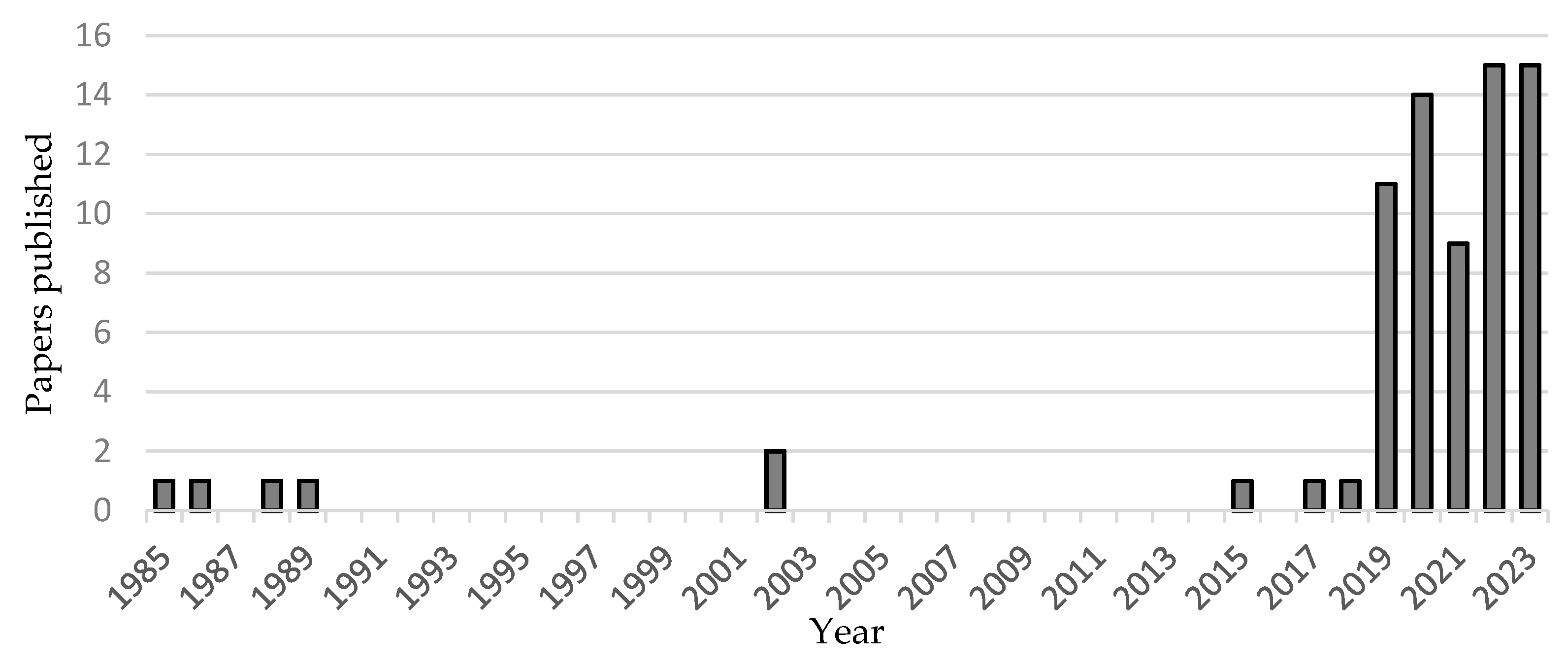
Figure 2.
Relation between the acquisition components and related parameters; in red the impact of the sample type, in green the resolution related parameters, in light blue the lighting, exposure, filter trio, in yellow the computer parameters, in purple the acquisition noise, and in dark blue the volume dilemma.

Figure 3.
Schema of the permanent mounting technique; (A) preparation before mounting; (B) epoxy application; and (C) the final result with removal of the slide.
Figure 3.
Schema of the permanent mounting technique; (A) preparation before mounting; (B) epoxy application; and (C) the final result with removal of the slide.

Figure 4.
Schema of the temporary mounting technique; (A) ethanol application; (B) grain mounting; and (C) grain recovery.
Figure 4.
Schema of the temporary mounting technique; (A) ethanol application; (B) grain mounting; and (C) grain recovery.

Figure 5.
Pico color gauge target by Image Science Associates (ISA); (A) schematic view of the color gauge with a grid and the theoretical value of each square using the Adobe RGB color space; (B) mosaic photomicrograph of the color gauge using the parameters detailed in Table 2. The 18% gray square is outlined by the red square in A and B.

Figure 6.
(A) Diagram of the BX53M installation, (B) the sample holder with the acrylic glass in light gray, (C) photograph of the BX53M installation, and (D) photograph of the BX53M microscope.
Figure 6.
(A) Diagram of the BX53M installation, (B) the sample holder with the acrylic glass in light gray, (C) photograph of the BX53M installation, and (D) photograph of the BX53M microscope.

Figure 7.
Warm-up period diagram (exposure time: 5.993 ms); temperature in yellow and the R, G, and B channel in red, green, and blue, respectively; (A) the test is performed with the microscope enclosure and (B) without enclosure.
Figure 7.
Warm-up period diagram (exposure time: 5.993 ms); temperature in yellow and the R, G, and B channel in red, green, and blue, respectively; (A) the test is performed with the microscope enclosure and (B) without enclosure.
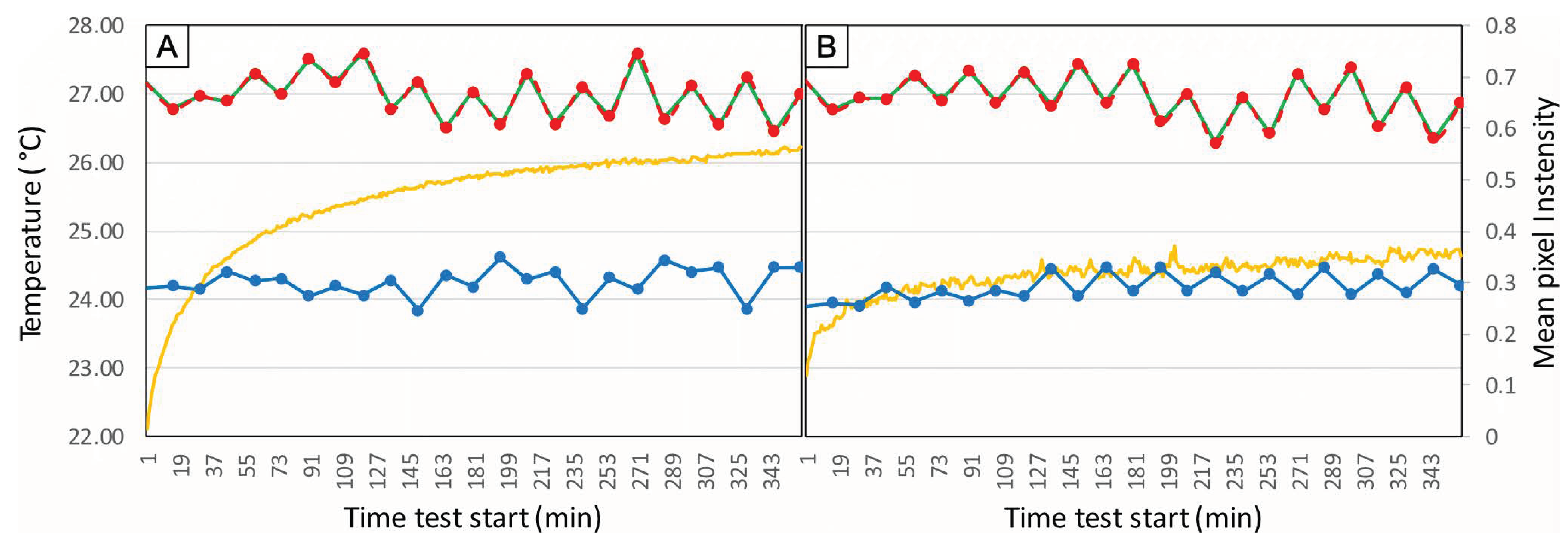
Figure 8.
Pixel intensity as a function of its theoretical intensity; (A) the grayscale squares population and (B) the color squares population.
Figure 8.
Pixel intensity as a function of its theoretical intensity; (A) the grayscale squares population and (B) the color squares population.
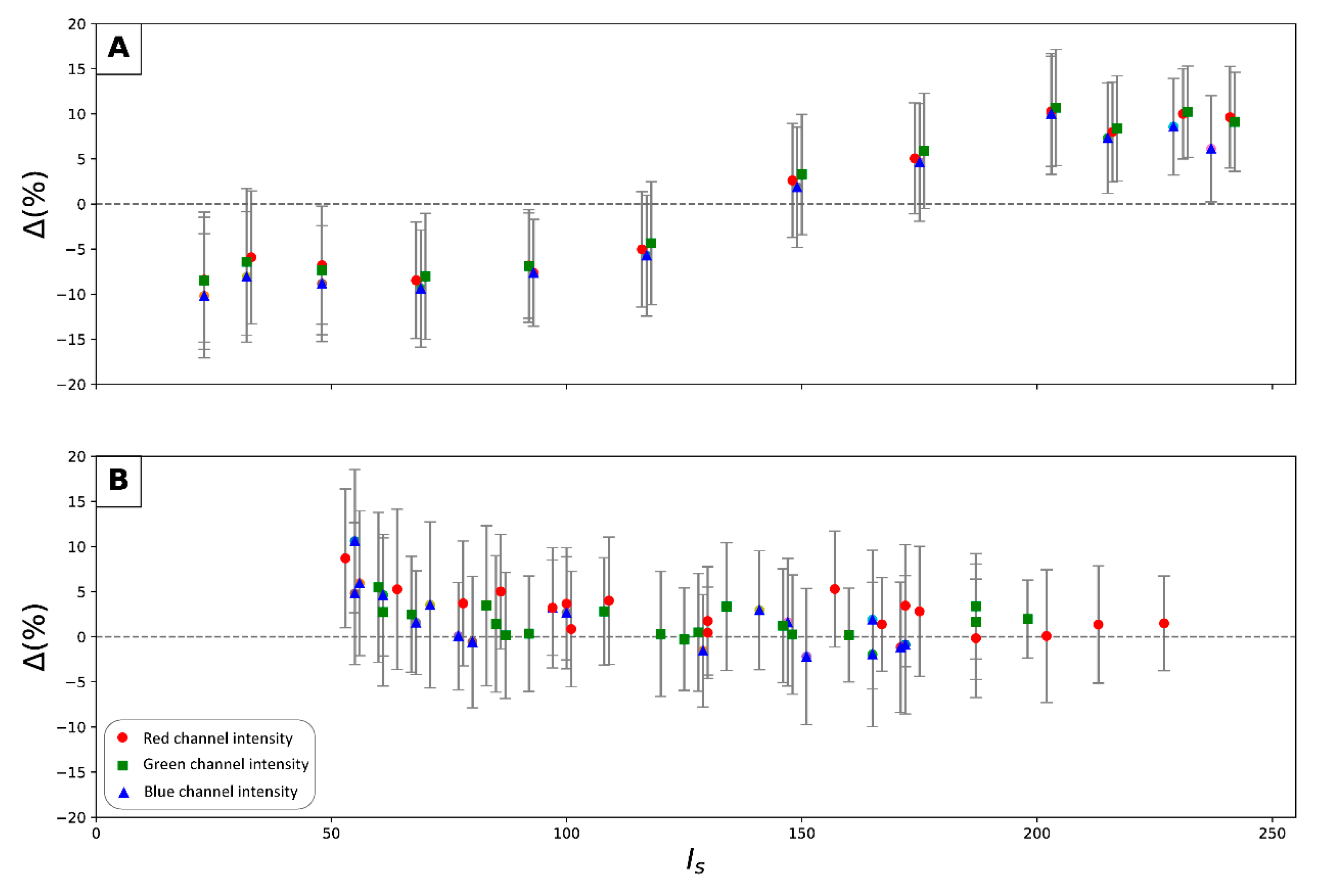
Figure 9.
Image of the same epidote grain acquired during the 8 tests.

Figure 10.
Mean intensity value of tests 2 and 3 against the mean intensity value of test 7, the black dashed line represents the y = x line and the grey dashed lines represent 5% variation from the y = x line, the first column is the channels of the red square image, the second for the green square and the third for the blue square, and the error bar is the standard deviation.
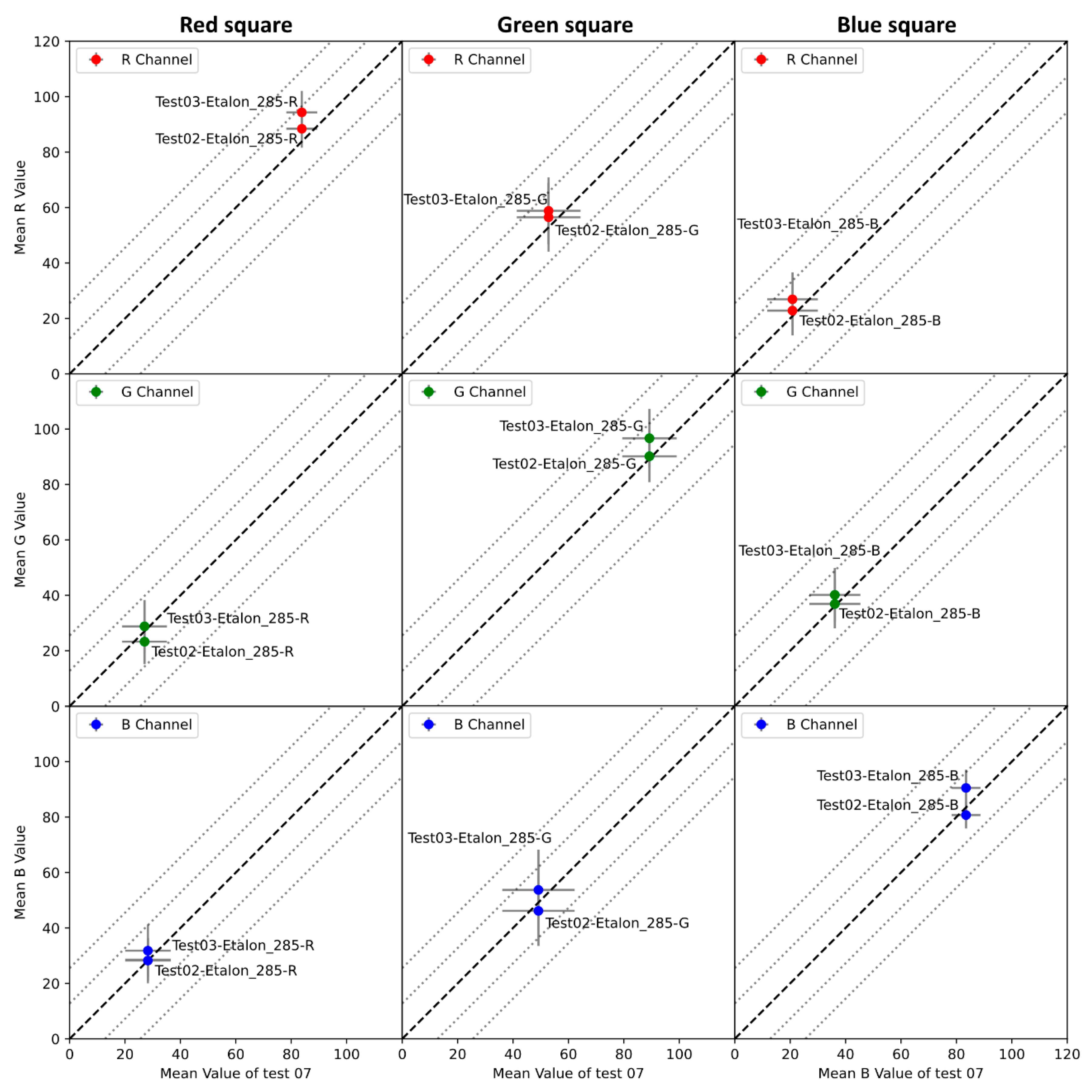
Figure 11.
Mean intensity value of tests 4 and 5 against the mean intensity value of test 7, the black dashed line represents the y = x line and the grey dashed lines represent 5% variation from the y = x line, the first column is the channels of the red square image, the second for the green square and the third for the blue square, and the error bar is the standard deviation.
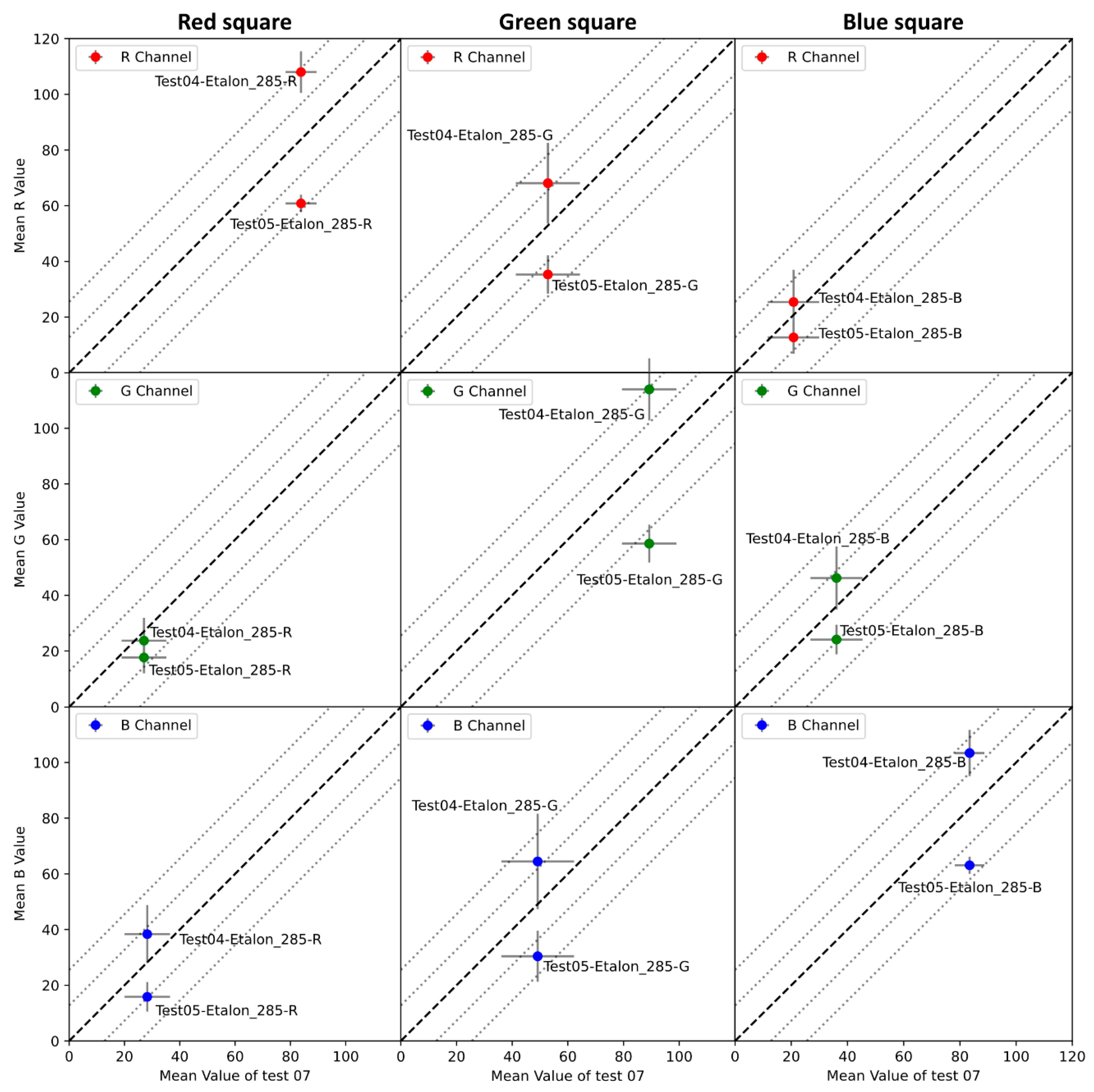
Figure 12.
Mean intensity value of the tests 1, 6, and 8 against the mean intensity value of test 7, the black dashed line represents the y = x line and the grey dashed lines represent 5% variation from the y = x line, the first column is the channels of the red square image, the second for the green square and the third for the blue square, the error bar is the standard deviation.

Figure 13.
The same epidote grain in each test series: (A) 05-07-2022 AL, (B) 06-07-2022 AL, (C) 07-07-2022 AL, (D) 08-07-2022 WP-100, (E) 08-08-2022 45K, and (F) 12-07-2022 75K.
Figure 13.
The same epidote grain in each test series: (A) 05-07-2022 AL, (B) 06-07-2022 AL, (C) 07-07-2022 AL, (D) 08-07-2022 WP-100, (E) 08-08-2022 45K, and (F) 12-07-2022 75K.
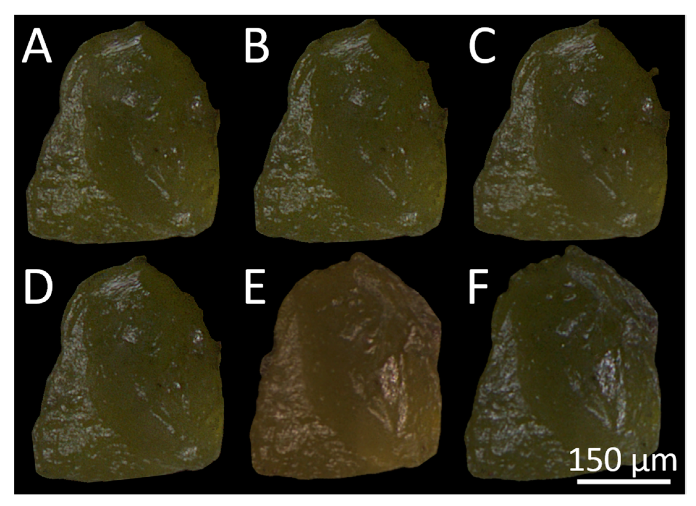
Figure 14.
Mineral proportions of the analyzed grains (A,C) and the relative difference in proportion per mineral (B,D). The gray shading reflects the error, represented as twice the relative standard deviation for the AL (green lines), WP-0 (blue lines), and WP-100 (yellow lines) series, each color line represents one acquisition. Proportions are used to avoid issues with differences in total grains among acquisitions.
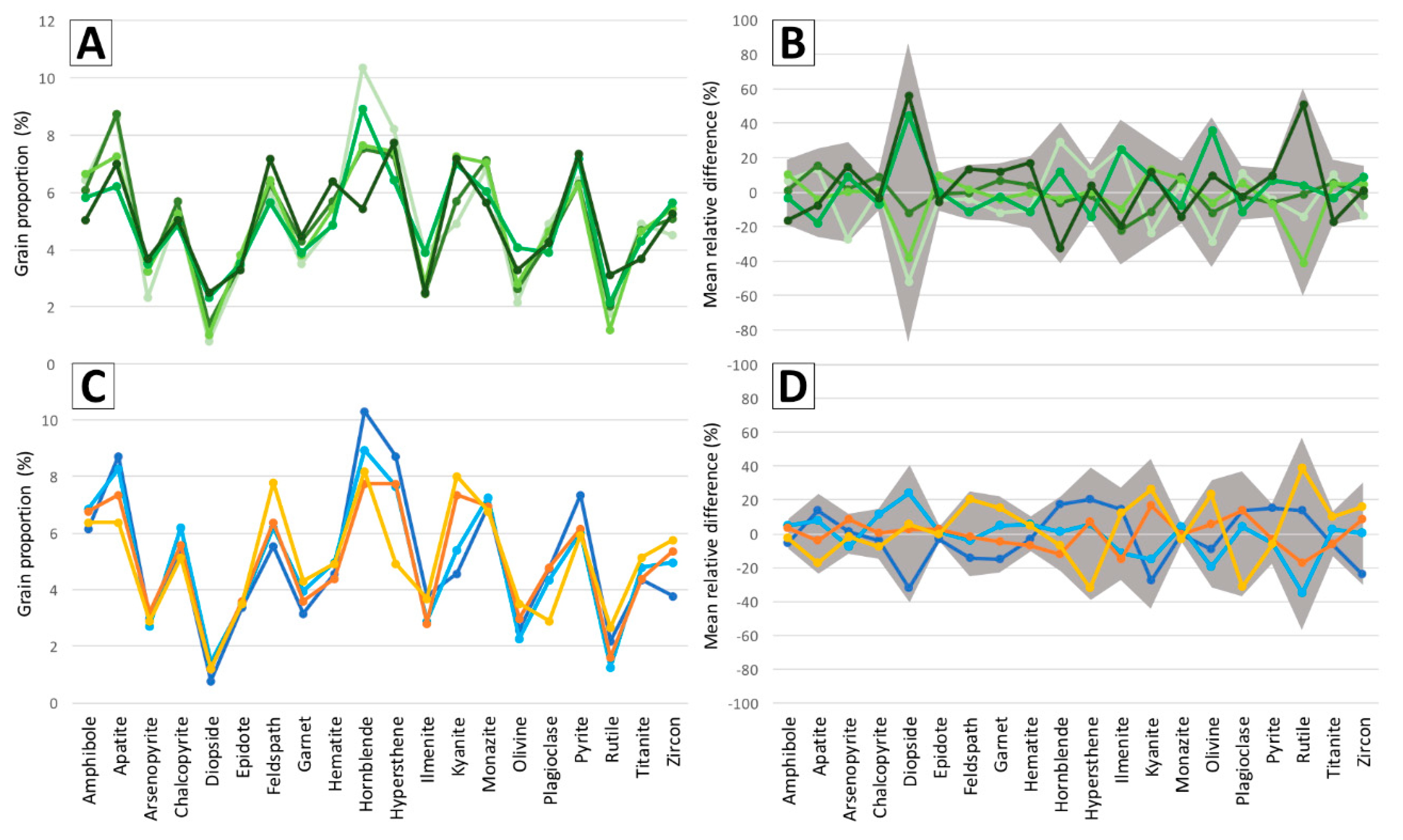
Figure 15.
Mineral proportions of the analyzed grains (A,C) and the relative difference in proportion per mineral (B,D). The gray shading reflects the error, represented as twice the relative standard deviation for the 45K (brown lines) and 75K (blue lines) series, each color line represents one acquisition.
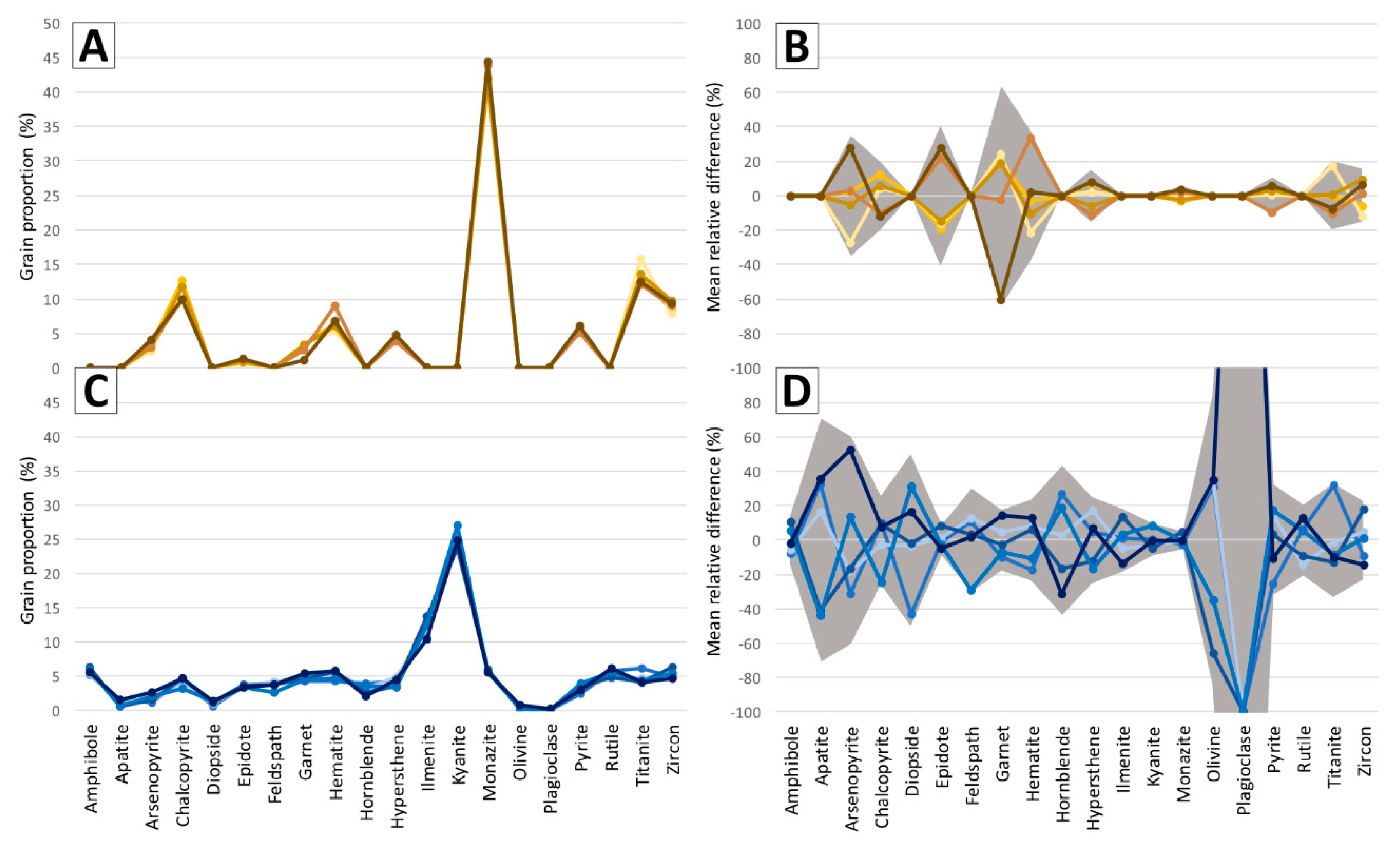

Table 1.
List of the acquisition parameters.
| Component | Details |
|---|---|
| Microscope | BX53M from Olympus |
| Camera | SC50 CMOS from Olympus |
| Objective | UPLFLN4XP from Olympus: and |
| Image resolution | 1920 × 2560 pixels |
| Exposure time | 5.993 ms |
| Color space | Adobe RGB |
| Light source type | Annular LED light |
| Light source intensity | Maximum |
| White balance | 18% gray square |
| Box enclosure | Yes |
| 20 |
Table 2.
Comparison of the characteristics of the permanent and temporary mounting techniques.
| Permanent | Temporary | |
|---|---|---|
| Mineral species for learning | Several per glass slide | One per glass slide |
| Mineral species to identify unknown | Several per glass slide | Several per glass slide |
| Manufacturing time | 24 to 48 h | Less than 10 min |
| Conservation | Permanent (vacuum proof) | Temporary |
| Lighting type | Transmitted light Reflected light Annular light Directional light | Transmitted light Reflected light Annular light Directional light |
| Polarization | Available | Available |
| Specific risk | Mounting failure | Visual sorting errors |
Table 3.
Number of grain photomicrographs per mineral used for the convolutional neural network (CNN) training.
Table 3.
Number of grain photomicrographs per mineral used for the convolutional neural network (CNN) training.
| Mineral | Training (1) | Validation (2) | Testing (3) | Total |
|---|---|---|---|---|
| Amphibole | 105 | 22 | 23 | 150 |
| Apatite | 98 | 21 | 21 | 140 |
| Arsenopyrite | 71 | 15 | 16 | 102 |
| Chalcopyrite | 57 | 12 | 12 | 81 |
| Diopside | 102 | 22 | 21 | 145 |
| Epidote | 105 | 22 | 23 | 150 |
| Feldspar | 70 | 15 | 15 | 100 |
| Garnet | 105 | 22 | 23 | 150 |
| Hematite | 74 | 16 | 16 | 106 |
| Hornblende | 55 | 12 | 11 | 78 |
| Hypersthene | 105 | 22 | 23 | 150 |
| Ilmenite | 105 | 22 | 23 | 150 |
| Kyanite | 105 | 22 | 23 | 150 |
| Monazite | 105 | 22 | 23 | 150 |
| Olivine | 105 | 22 | 23 | 150 |
| Plagioclase | 105 | 22 | 23 | 150 |
| Pyrite | 105 | 22 | 23 | 150 |
| Rutile | 40 | 9 | 8 | 57 |
| Titanite | 90 | 19 | 20 | 129 |
| Zircon | 89 | 19 | 19 | 127 |
Table 4.
Acquisition parameter tests description.
| Test | Parameter Variation | Respect Pirard’s Protocol (without Correction) |
|---|---|---|
| Test 1 | No warming period | No |
| Test 2 | No microscope enclosure and incandescent room lighting | Yes |
| Test 3 | No microscope enclosure and LED room lighting | Yes |
| Test 4 | Exposure time change: 8.991 ms | No |
| Test 5 | Exposure time change: 2.996 ms | No |
| Test 6 | Medium light intensity | No |
| Test 7 | Protocol fully respected | Yes |
| Test 8 | Medium light intensity, exposure time of 8.991 ms | No |
Table 5.
Mean R, G, and B intensity values with standard deviation of images in Figure 13.
Table 5.
Mean R, G, and B intensity values with standard deviation of images in Figure 13.
| Image | Mean R Intensity Value | Mean G Intensity Value | Mean B Intensity Value |
|---|---|---|---|
| A | 50.55 ± 30.61 | 48.52 ± 29.95 | 26.94 ± 21.13 |
| B | 49.30 ± 30.27 | 47.37 ± 29.61 | 25.36 ± 20.22 |
| C | 48.96 ± 30.17 | 46.80 ± 29.34 | 26.41 ± 20.60 |
| D | 48.97 ± 30.09 | 46.77 ± 29.26 | 26.80 ± 21.01 |
| E | 45.99 ± 35.38 | 38.05 ± 29.63 | 19.76 ± 17.80 |
| F | 42.43 ± 32.52 | 41.34 ± 32.10 | 27.08 ± 24.33 |
Disclaimer/Publisher’s Note: The statements, opinions and data contained in all publications are solely those of the individual author(s) and contributor(s) and not of MDPI and/or the editor(s). MDPI and/or the editor(s) disclaim responsibility for any injury to people or property resulting from any ideas, methods, instructions or products referred to in the content. |
© 2023 by the authors. Licensee MDPI, Basel, Switzerland. This article is an open access article distributed under the terms and conditions of the Creative Commons Attribution (CC BY) license (https://creativecommons.org/licenses/by/4.0/).
Share and Cite
MDPI and ACS Style
Back, A.L.; Bédard, L.P.; Maitre, J.; Bouchard, K. From Rocks to Pixels: A Protocol for Reproducible Mineral Imaging and its Applications in Machine Learning. Minerals 2024, 14, 51. https://doi.org/10.3390/min14010051
AMA Style
Back AL, Bédard LP, Maitre J, Bouchard K. From Rocks to Pixels: A Protocol for Reproducible Mineral Imaging and its Applications in Machine Learning. Minerals. 2024; 14(1):51. https://doi.org/10.3390/min14010051
Chicago/Turabian StyleBack, Arnaud L., L. Paul Bédard, Julien Maitre, and Kévin Bouchard. 2024. "From Rocks to Pixels: A Protocol for Reproducible Mineral Imaging and its Applications in Machine Learning" Minerals 14, no. 1: 51. https://doi.org/10.3390/min14010051
Note that from the first issue of 2016, this journal uses article numbers instead of page numbers. See further details here.