An Automated Approach to the Heterogeneity Test for Sampling Protocol Optimization

Abstract

The fundamental sampling error is one of the sampling errors defined by Pierre Gy’s Theory of Sampling and is related to the constitution heterogeneity of the mineralisation. Even if a sampling procedure is considered ideal or perfect, this error will still exist and, therefore, cannot be eliminated. A key input into Gy’s fundamental sampling error equation is intrinsic heterogeneity. The intrinsic heterogeneity of a fragmented lot can be estimated by the “calibrated” formula of Gy, which can be written as a function of the sampling constants K and α. These constants can be calibrated by the standard heterogeneity test, originally developed by Pierre Gy and Francis Pitard. This method is based on the selection of rock fragments, individually and randomly, in an equiprobabilistic way from a lot of particulate material, aiming to estimate the intrinsic heterogeneity of the lot. This test, in addition to demanding time and space, can be influenced by human biases, and is difficult to quantify or measure. Aiming to simplify the test execution and eliminate the variance generated by human biases, a prototype called the intrinsic heterogeneity tester was developed as an automated alternative for heterogeneity testing. This prototype selects fragments from a falling stream, one by one, by means of a predefined laser count. To evaluate the prototype, a study was carried out, using painted chickpeas to simulate mineralisation grades and, sequentially, processing the same lot in the intrinsic heterogeneity tester prototype several times. The statistical and mineral content analysis, and comparisons between the intrinsic heterogeneity tester and the standard heterogeneity test sampling constants and constitution heterogeneities were undertaken. As a result, the authors conclude that the intrinsic heterogeneity tester prototype can be used as an alternative to the manual selection of individual fragments and for estimating the intrinsic heterogeneity of particulate material lots to support sampling protocol optimization.

1. Introduction

1.1. Overview of Sampling

The mining value chain includes sample collection, preparation, and analysis processes, as well as geometallurgical, physical, and chemical tests. These processes form the basis for estimating the mineral resources, masses, and grades of mineralisation and their performance in the processing plant. The importance of sampling in mining from exploration to the final product is undeniable [1].

Samples can be made up of in situ material, comminuted rocks, or drill cores. In any case, the objective is to obtain a representative sample that accurately describes the material, or lot, in question. The collection of samples in the field is followed by a process of reduction both in mass and particle size, so that tests and analyses can then be carried out. This process can become complex, especially for some very heterogeneous mineralisation such as gold [2].

1.2. Theory of Sampling

1.2.1. Background

Dr Pierre Gy’s Theory of Sampling (TOS) [3,4,5,6] aims to control the sampling processes so that the results are unbiased and precise. Thus, if the sampling process respects the scientific aspects and predetermined parameters of the TOS, guaranteeing the absence of systematic errors, there will still be an error called the fundamental sampling error (FSE) which is related to the constitution heterogeneity (CH) of the mineralisation. The FSE is due to the difference between the real grade of the lot and the grade of the sample collected to represent that lot or population. FSE is considered the smallest existing error when the sampling process is ideal, that is, when the sample fragments are equiprobably collected, one by one, at random [3,4,5,6,7].

Since the TOS was created, several authors have discussed how to estimate the intrinsic heterogeneity (IH) of different types of mineralisation comminuted to different particle sizes, aiming to calculate the FSE of each sampling stage. Gy initially proposed estimating the so-called “constant factor of constitution heterogeneity” or “intrinsic heterogeneity of the lot” (IH_L) by multiplying specific factors defined for each mineralisation type [8,9]. Then, in his 1988 and 1992 books [10,11], he introduced the first heterogeneity test (HT) to calculate an experimental estimate of IH_L, EST[IH_L], called the “50/100 fragment method”, where the operator should collect, one by one, randomly, at least 50, preferably 100, fragments belonging to the coarsest size class of the lot of material under study, then wash, weigh, and analyse each fragment for all critical components. This method was then adapted into the so-called “Modified 50-piece test” [12], which suggests that it is the practitioner’s decision to either select 50 individual fragments or 50 groups of individual fragments, each group composed of an equal number of fragments, selected one by one, randomly. Other authors proposed the calibration of IH_L based on similar HTs, from which the two sampling parameters or sampling constants, K and α, are derived [13,14,15]. Based on the work from these authors, IH_L can be calculated as a function of the top-size, or d₉₅, of the fragments (d), as for Equation (1).

$${\mathrm{I}\mathrm{H}}_{\mathrm{L}}=\mathrm{K}{\mathrm{d}}^{\mathsf{\alpha }}.$$

(1)

By estimating IH_L, it is possible to calculate the variance of the FSE (Equation (2), also known as the “calibrated Gy’s formula”) and, consequently, determine the minimum representative sample masses and optimize sampling protocols.

$${{\mathrm{s}}_{\mathrm{F}\mathrm{S}\mathrm{E}}^2=\mathrm{K}\mathrm{d}}^{\mathsf{\alpha }}\left(\frac{1}{{\mathrm{M}}_{\mathrm{s}}}-\frac{1}{{\mathrm{M}}_{\mathrm{L}}}\right).$$

(2)

where ${\mathrm{s}}_{\mathrm{F}\mathrm{S}\mathrm{E}}^2$ is the variance of the FSE, K and α are the sampling constants, M_S is the sample mass, and M_L is the lot mass.

There is more than one methodology for deriving the K and α sampling constants: the HT [3], the sampling tree experiment (STE) [13], and the segregation free analysis (SFA) [14,15].

1.2.2. Intrinsic Heterogeneity

Intrinsic heterogeneity (IH), or CH, is the component of heterogeneity driven by differences in particle size and variation in composition between one particle and another. The greater the difference between the amount of target analyte (or content) in the particles, the greater the IH value. For example, a jar containing white marble pebbles of the same size, mass, and chemical composition has an IH of zero. A jar containing white and black marble pebbles of the same size has a positive IH. The IH cannot be negative because it is a variance [16].

1.2.3. Standard Heterogeneity Test

The standard HT consists of manually collecting random fragments, one by one, individually, from a lot of particulate material, simulating an ideal sampling procedure. The procedure is performed for different size fractions to obtain the calibrated sampling constants K and α. The material of each size fraction is evenly spread on a grid drawn on a table or flat surface, so that all fragments are accessible and have similar probabilities of selection. The first subsample is composed of one fragment, randomly collected from each cell of the grid, making up n-fragment subsample, as n is the number of cells. This procedure is repeated at least 50 times, generating 50 subsamples of n fragments for each size fraction [15].

The initial condition for a lot to be suitable for heterogeneity testing is:

$$\mathrm{n}>10\times \mathrm{Q}\times \mathrm{p}.$$

(3)

That is, the number of fragments—n—present in each size fraction must be greater than 10 times the number of collected groups—p—multiplied by the number of fragments—Q—collected per group [3].

After collecting the subsamples, the groups are weighed and chemically analysed.

1.3. Aim of This Paper

Performing the standard HT is complex and demands a lot of time and physical space to complete [1,2,15,17]. This is the reason why several authors have proposed simplified versions of the test [13,14,15], which sometimes present similar and satisfactory results, but most times does not. It is important to point out that none of the simplified versions proposed by these authors make the individual and random selection of fragments, but make the division using riffle or rotating splitters, generating an additional variance to the results: the variance of the grouping and segregation error (GSE).

The IHT prototype presented in this paper was developed to carry out the random and individual selection of fragments, as proposed by the standard HT.

The study presented—named the “Chickpea Study”—arose, therefore, from the need to validate the IHT as an adequate and unbiased prototype for carrying out the HT through statistical analysis. The IHT system aims to provide a quicker, cheaper, and more effective method for IH_L determination, which, importantly, allows for larger and multiple tests where appropriate.

2. Materials and Methods

2.1. Introduction

This section provides a detailed description of the IHT prototype, highlighting its technical features and operational functionality. The study conducted, referred to as the Chickpea Study, aimed to validate the performance of the IHT. The Chickpea Study will be detailed, addressing the experimental procedures and metrics.

2.2. The Prototype

The prototype developed to automate the HT can be seen as a robot (Figure 1) composed of:

• A rotating wooden wheel with a diameter equal to 130 cm;
• Four plastic wheels with a diameter of 5 cm which rotate the table;
• A wooden table 175 cm long and 72 cm wide;
• Two easels 80 cm high, 80 cm wide and 45 cm wide;
• 50 containers (cups) of 150 mL made of transparent plastic;
• 50 wooden cubes with 2 cm edges;
• A 10-L plastic container for material storage (‘storage container’);
• Two hollow wooden cubes with 32 cm edges;
• A hollow wooden cube with 40 cm edges;
• Two square wooden sheets measuring 32 cm with a thickness of 2 cm;
• A 54 cm metal trough (‘vibrating feeder’);
• A 15 cm hollow glass parallelepiped (‘free-fall duct’);
• Two blades for directing fragments (‘deflector blade’) and locking the table;
• Three 5 cm PVC tubes;
• A laser emitter and receiver;
• Two mirrors;
• A power supply;
• Two digital counters;
• Two digital counters with preset;
• A computer cooler;
• A switch.

The unit operation is described as follows.

A lot of particulate material to be tested, belonging to a given size fraction, is placed inside the 10 L storage container. The prototype switch turns on the laser and the power supply. When turning on the power supply, the counters are activated, and the vibration starts so that the fragments are directed in line until the end of the vibrating feeder, which has a capacity of 0.4 L.

As the fragments fall, passing through the laser beams, the partial counter starts counting until it reaches the number “n” predefined by the operator. It immediately activates the deflector blade to direct the n^th fragment to the plastic cup positioned under the sample discharge. The remaining fragments are directed to the reject discharge.

The partial counter informs the total counter that the fragment has been collected and activates the wooden wheel motor, turning the wheel and directing the next plastic cup under the sample discharge. This process is repeated until the operator-defined number of fragments for each cup is reached, then the total fragment counter turns off the power supply.

In the test case presented here, the predefined partial counter is set to 10 fragments (i.e., the collection of 1 fragment for every 10 that pass through the laser counter), and the total counter to 100 (i.e., the collection of 100 fragments in total or two fragments in each of the 50 cups). In this case, when the prototype is turned on and the feeder starts to vibrate, the fragments start to fall and the partial counter starts to count. When the 10th fragment passes through the laser, the deflector blade directs the fragment to the sample discharge which feeds the first plastic cup, and immediately the wheel motor turns the table, positioning the second cup below the sample discharge. Simultaneously, the partial counter informs the total counter that the count has reached 10. At this point, the total counter shows “1”, and the partial counter restarts counting from 0 until it reaches 10 again and collects the second fragment, when the total counter shows “2”. This procedure is repeated until the total counter reaches 100 (i.e., 100 fragments collected). At the end of this test, each of the 50 plastic containers should contain two fragments. Figure 2 shows the prototype performing a test with mineral fragments.

2.3. The Chickpea Study

2.3.1. Parameters Applied

The Chickpea Study aimed to analyse the variance of the same lot that goes through the same sampling process several times. It is not possible to carry out this test with mineralised material, since the chemical preparation and analysis processes are destructive and do not allow for the test to be repeated with the same material. Furthermore, grains are particles with similar mass and size, which can be painted for simulating different grades that can be calculated by counting the number of particles of different colours. In this way, the test can be conducted with the same lot as many times as necessary.

Many types of grains were tested, and among them, the chickpea was chosen due to its rough surface and a diameter of approximately 12 mm, and characteristics closer to mineralised fragments coming from mineral processing plant feeds than the other grains like beans, fava beans, and rice, smaller and with smoother surfaces. It is important to highlight that the IHT unit operates in the particle size range of 3.35 mm to 19.0 mm.

The primary chickpea sample contained 25,460 g. To estimate the mass of each particle, 100 groups of 10 unpainted particles were weighed, which resulted in an average particle mass of 0.57113 g. Through the estimated mass of a particle, the total number of particles was calculated, which was approximately 44,578 particles.

Following the recommendations of the HT (Section 1.2.3), the prototype selection method was set to collect 1 particle every 10 particles. Based on the available quantity of chickpeas, the estimated number of particles per group, or the number of particles in each plastic cup, was defined by dividing the total number of particles (44,578) by the product of the number of groups (50) and the initial condition for HTs (10, as the number of fragments must be 10 times greater than the number of collected particles):

$$Estimated number of particles per group=\raisebox{1ex}{$\mathrm{44,578}$}\!\left/ \!\raisebox{-1ex}{$50\times 10$}\right.=89.2.$$

However, to ensure that the robot did not run out of particles before the test is over, it was decided to set up the IHT prototype so that each of the 50 groups was made of 88 particles. It is important to point out that, ideally, 100% of the initial lot was to be used in the tests.

2.3.2. Test L

The first test performed was called “Test L” (‘L’ for ‘low grade’) and aimed to simulate a low-grade mineralisation. Fifty particles were taken from the lot, painted blue and returned to the lot (Figure 3). The lot was mixed and placed in the storage container.

Considering the 50 blue painted particles, the estimate content of the lot with blue particles was 0.112%. The summary of Test L parameters is shown in

Table 1. Test L parameters.

Test L—Parameters
Estimated number of particles per group	88
Particle mass (g)	0.57113
Total mass (g)	25,460
Estimated total number of particles	44,578
Number of groups	50
Estimated number of particles collected	4400
Particle collection	1 in 10
Blue content (%)	0.11%

.

Test L was performed three times with the same primary lot. The tests were named L01, L02, and L03. Figure 4 shows the 50 chickpea subsamples generated by Test L01, with 1 blue particle in the subsamples number 1, 9, 12, 23, and 38. During the three tests, the feeder vibration was controlled according to the flow intensity, that is, when the movement of the particles in the feeder was slow, the vibration was increased, and when the movement was fast, the vibration was reduced. This procedure was carried out so that the flow was constant most of the time. The detailed results of Test L are presented in Appendix A.

2.3.3. Test P

The second test performed was called “Test P” (for polymetallic mineralisation) and aimed to simulate a real polymetallic Cu-Pb-Zn deposit in Brazil. For this test, chickpea particles were painted by the mass (Figure 5). The mass of white particles was 2637.58 g, the orange particle mass was 3726.93 g, and the red particle mass was 260.44 g. Considering these masses, the estimated white “mineral” content was 10.36%, the orange “mineral” content was 14.64%, and the red “mineral” content was 1.02%. It is important to emphasise that, despite their appearance in the photograph, the blue particles are not part of the Test P.

As in Test L, each of the 50 groups was composed of 88 particles. The summary of Test P parameters is shown in

Table 2. Test-P parameters.

Test P—Parameters
Estimated number of particles per group	88
Particle mass (g)	0.57113
Total mass (g)	25,460
Estimated total number of particles	44,578
Number of groups	50
Estimated number of particles collected	4400
Particle collection	1 in 10
White content (%)	10.36%
Orange content (%)	14.64%
Red content (%)	1.02%

.

Test P was performed three times with the same primary lot. The tests were named P01, P02, and P03. Unlike Test L, the feeder vibration remained constant during each test. Therefore, it is possible to evaluate the impact of changes in particle flow, as it varies throughout the test when the vibration remains constant. The vibration can be controlled by the power supply voltage (U), and the voltages used were set as follows:

• Test P01: U = 6.7 V;
• Test P02: U = 7.2 V;
• Test P03: U = 6.5 V.

The detailed results of Test P are presented in Appendix B.

It is important to emphasize that, when the feeder vibration is constant, the flow of the particles oscillates. Therefore, it was decided not to adjust this speed during each of the three tests, aiming to: (i) verify whether the robot could work during the entire test without human intervention and; (ii) verify the influence of the feeder vibration on the particle selection.

3. Results and Discussion

3.1. Introduction

The discussion was divided into three stages:

• Validation of the results from the Test L which simulates low-grade mineralisation, statistically based on the binomial distribution;
• Validation of the results from the Test P which simulates polymetallic mineralisation, also statistically based on the binomial distribution;
• Calculation and comparison of the IHL with mineralised material results.

It is important to point out that the binomial distribution is commonly used to model scenarios involving binary outcomes. It is a discrete probability distribution of the number of successes in a fixed number of independent Bernoulli trials, where each trial has only two possible outcomes: success or failure [16]. In the context of the study, it serves as a statistical framework for assessing the validity of the test results by quantifying the likelihood of obtaining a certain number of successes given the parameters of the test conditions.

3.2. Test L

When a set of independent trials have probability $\mathrm{p}$ of success and $(1-\mathrm{p})$ of failure, the results follow a binomial distribution [16]. For the tests carried out in this study, the particles have or do not have colour, so this is the distribution represented here.

For a group of 44,578 particles with 50 blue particles, the probability of success calculation [16] is given below:

$$\mathrm{p}=\frac{50}{\mathrm{44,578}}\times 100\approx 0.112\mathrm{\%}.$$

The expected value of successes ($\mathrm{E}\left\{\mathrm{J}\right\}$) and the variance ($\mathrm{v}\mathrm{a}\mathrm{r}\left\{\mathrm{J}\right\}$) are:

$$\mathrm{E}\left\{\mathrm{J}\right\}=\mathrm{n}\mathrm{p}\approx 4400\times 0.00112\approx 4.9352.$$

$$\mathrm{v}\mathrm{a}\mathrm{r}\left\{\mathrm{J}\right\}=\mathrm{n}\mathrm{p}(1-\mathrm{p})\approx 4400\times 0.00112\times (1-0.0011)\approx 4.9296.$$

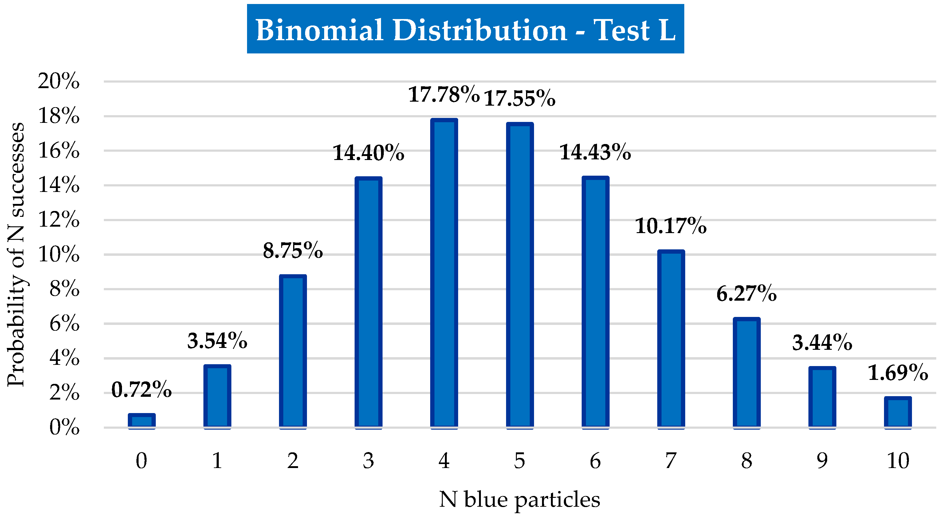
Figure 6 shows the results of the probability density function [16] for Test L. It is possible to observe that the highest probability of success is in the selection of 4 or 5 blue particles, which are the integer values around the expected value of 4.9352.

Table 3. Test L experimental results.

Results	Test L01	Test L02	Test L03
Particles collected	4537	4468	4523
Blue particles collected	5	4	5
Maximum particle per sample	96	94	96
Minimum particle per sample	87	85	85
Average particle per sample	90.74	89.36	90.46
Variance	3.6724	3.4704	5.4884
Relative variance	0.000446	0.000435	0.000671
Standard deviation	1.94	1.88	2.37
Coefficient of variation	2.13%	2.11%	2.62%

summarizes the results of the Tests L01, L02, and L03.

Table 3 shows that the 50 subsamples, when considered as a single sample, represented very closely the original lot. With the selection of five blue particles in Tests L01 and L03, and four blue particles in Test L02, the integer values projected with greater probability by the binomial distribution. It is important to note that the particles either contain or do not contain colour, so the results will always present integer values. Furthermore, the observed number has a variance close to the expected value (4.9352), which must be considered when analysing the results.

It is important to note that, not infrequently, two particles were collected at once, and some particles were thrown out of the robot by the deflector blade. These problems, especially the selection of two particles at once, directly affected the number of particles per cup, which was often above 88. This interference is evident in the descriptive statistics results, as seen in the total number of collected particles (above 4400) and the number of particles per subsample (not always 88).

Based on the descriptive statistics data, it is possible to observe that the tests have similar coefficients of variation (CV). Conservatively, the highest CV was considered as the precision measure of the IHT prototype for Test L, i.e., 2.62%.

The precision (comparison between the Tests L01, L02, and L03) and accuracy (comparison of L01, L02, and L03 with the lot) measurements, that is, the representativeness of the selection of coloured particles, was carried out through the analysis of “mineral” content, where the similarity of values was observed (

Table 4. Test L—“mineral” content analysis.

Content Analysis
Test L01	0.11%
Test L02	0.09%
Test L03	0.11%
Lot	0.11%

).

It is worth emphasising that each subsample cannot represent the lot and, this is not the objective of HTs. Nevertheless, the 50 subsamples, when considered as a single sample, represented the original lot very closely, as shown in Table 4. The variance between the subsamples can be seen as the IH of the lot.

3.3. Test P

3.3.1. Red Particle Distribution

For a group of 25,460 g with 260.44 g of red particles, the probability of success calculation [16] is given by:

$$\mathrm{p}=\frac{260.44}{\mathrm{25,460}}\times 100\approx 1.023\%.$$

The expected value of successes ($\mathrm{E}\left\{\mathrm{J}\right\}$) and the variance ($\mathrm{v}\mathrm{a}\mathrm{r}\left\{\mathrm{J}\right\}$) are:

$$\mathrm{E}\left\{\mathrm{J}\right\}=\mathrm{n}\mathrm{p}\approx 4400\times 0.01023\approx 45.0093.$$

$$\mathrm{v}\mathrm{a}\mathrm{r}\left\{\mathrm{J}\right\}=\mathrm{n}\mathrm{p}(1-\mathrm{p})\approx 4400\times 0.0102\times (1-0.0102)\approx 44.5489.$$

Figure 7 shows the results of the probability density function [16] for Test P—red particles. It is possible to observe that the highest probability of success is in the interval of 44 and 46 particles, which is the interval of the graph that contains the expected value of 45.0093.

3.3.2. White Particle Distribution

For a group of 25,460 g with 2637.58 g of white, the probability of success calculation [16] is given by:

$$\mathrm{p}=\frac{2637.58}{\mathrm{25,460}}\times 100\approx 10.360\mathrm{\%}.$$

The expected value of successes ($\mathrm{E}\left\{\mathrm{J}\right\}$) and the variance ($\mathrm{v}\mathrm{a}\mathrm{r}\left\{\mathrm{J}\right\}$) are:

$$\mathrm{E}\left\{\mathrm{J}\right\}=\mathrm{n}\mathrm{p}\approx 4400\times 0.1036\approx 455.8269.$$

$$\mathrm{v}\mathrm{a}\mathrm{r}\left\{\mathrm{J}\right\}=\mathrm{n}\mathrm{p}(1-\mathrm{p})\approx 4400\times 0.1036\times (1-0.1036)\approx 408.6046.$$

Figure 8 shows the results of the probability density function [16] for Test P—white particles. It is possible to observe that the highest probability of success is in the interval of 450 and 460 particles, which is the interval of the graph that contains the expected value of 455.8269.

3.3.3. Orange Particle Distribution

For a group of 25,460 g with 3726.93 g of orange particles, the probability of success calculation [16] is given by:

$$\mathrm{p}=\frac{3726.93}{\mathrm{25,460}}\times 100\approx 14.638\mathrm{\%}.$$

The expected value of successes ($\mathrm{E}\left\{\mathrm{J}\right\}$) and the variance ($\mathrm{v}\mathrm{a}\mathrm{r}\left\{\mathrm{J}\right\}$) are:

$$\mathrm{E}\left\{\mathrm{J}\right\}=\mathrm{n}\mathrm{p}\approx 4400\times 0.1464\approx 644.0885.$$

$$\mathrm{v}\mathrm{a}\mathrm{r}\left\{\mathrm{J}\right\}=\mathrm{n}\mathrm{p}(1-\mathrm{p})\approx 4400\times 0.1464\times (1-0.1464)\approx 549.8044.$$

Figure 9 shows the results of the probability density function [16] for Test P—orange particles. It is possible to observe that the highest probability of success is in the interval of 640 and 650 particles, which is the interval of the graph that contains the expected value of 644.0885.

3.3.4. Experimental Tests Results

Table 5. Test P experimental results.

Results	Test P01	Test P02	Test P03
Particles collected	4436	4527	4512
Red particles collected	42	37	39
White particles collected	452	424	446
Orange particles collected	607	611	646
Maximum particle per sample	96	97	94
Minimum particle per sample	87	86	87
Average particle per sample	90.74	90.54	90.24
Variance	3.6724	4.5684	2.8624
Relative variance	0.00014	0.00057	0.00036
Standard deviation	1.05	2.16	1.71
Coefficient of variation	1.18%	2.38%	1.89%

summarises the results of the tests P01, P02, and P03.

Test P was conducted with three constant and distinct voltages applied to the power supply, which is the primary factor responsible for the vibrating feeder. It is important to note that the vibration undergoes slight variations depending on the amount of material present in the storage container. Therefore, during Tests L01, L02, and L03, the voltages were manually adjusted throughout the sampling process. For Tests P01, P02, and P03, the voltages varied, as discussed in Section 2.3.3.

The voltage for Test P01 (6.7 V) was chosen because it was the most frequently used voltage throughout the other tests. From this, a slightly higher and a slightly lower voltage were selected. The voltages were set before the start of the test, and some interferences in the process were observed, including:

• A full storage container slowed down the process, while an empty storage container made it faster, as expected;
• In Test P02, where the voltage was higher (7.2 V), particles tended to accumulate in the feeder, causing them to fall together through the free-fall duct;
• In Test P03, where the voltage was lower (6.5 V), particles were less affected by the vibration and could sometimes accumulate and fall together through the free-fall duct;
• Depending on the falling speed of the particles and their point of contact with the deflector blade, they were occasionally thrown out of the robot through the free-fall duct.

As observed in Test L, particles falling together directly affects the number of particles in each cup. This interference is evident in the descriptive statistics results.

Based on the descriptive statistics data, it is possible to observe that the tests have similar coefficients of variation (CV). Conservatively, the highest CV was considered as the precision measure of the IHT prototype for Test P, i.e., 2.38%.

The precision (comparison between the Tests P01, P02, and P03) and accuracy (comparison of P01, P02, and P03 with the lot) measurements, that is, the representativeness of the selection of coloured particles, was carried out through the analysis of “mineral” content, where the similarity of values was observed (

Table 6. Test P—“mineral” content analysis.

Content Analysis
	Red	White	Orange
Test P01	0.95%	10.19%	13.68%
Test P02	0.82%	9.37%	13.50%
Test P03	0.86%	9.88%	14.32%
Lot	1.02%	10.36%	14.64%

).

Note that each subsample does not represent the lot. Nevertheless, the 50 subsamples, when considered as a single sample, represented very closely the original lot, as shown in Table 6. The variance between the subsamples can be seen as the IH of the lot.

Finally, it is worth emphasizing that for Test P, differently from Test L, the lot grade was calculated by mass of particle groups, while the grades of the 50 subsamples were calculated by particle count. This difference in grade calculation (mass vs. particle counting) resulted in Test P subsamples presenting a trend of grade underestimation. This can be explained by the following analysis: 100 groups of 10 coloured particles were weighed, resulting in an average mass of the coloured particles of 0.58215 g, which is approximately 2% higher than the average mass of the uncoloured particle (0.57113 g). This difference alone justifies the subsample underestimated grades, since when calculating the grade by counting particles, the coloured particle (“mineral” of interest) is not considered to be heavier. Therefore, the sample grades shown in Table 6 are even closer to the lot grades. However, this problem will not occur in tests carried out with mineralised samples, whose grades are calculated by chemical analysis.

It is important to note that the initial grade is calculated by mass due to the large number of particles representing each grade when simulating polymetallic mineralisation. Therefore, it would be impractical, in terms of time to perform an initial one-by-one grade count.

It is noted that Test P subsamples present a trend of grade underestimation. This can be explained by the following analysis: 100 groups of 10 coloured particles were weighed, resulting in an average mass of the coloured particle of 0.58215 g, which is approximately 2% higher than the average mass of the uncoloured particle (0.57113 g). This difference alone justifies the subsample underestimated grades, since when calculating the grade by counting particles, it is not considered that the coloured particle (mineral of interest) is heavier. Therefore, the sample grades shown in Table 6 are even closer to the lot grades.

3.4. Calculation of IH_L

A number of publications discuss the relative pros and cons of the heterogeneity test work [13,14,15,18,19,20,21,22,23,24,25,26] using the simplified method for IH_L estimation described by Pitard (Chapter 11) [3]. It is not the authors’ intention to detail or judge the theoretical fundamentals of this approach. However, one of the reasons for using this method is that there is no need to calculate the liberation factor—one of the most debatable factors in the TOS [27]. For the Chickpea Study, the liberation factor is 1, as all “minerals” are liberated, which makes this estimation method suitable for this study.

Once the 50 subsamples generated by the HT are weighted and analysed, the mass M_q (given in grams) and grade a_q (given in decimals) for each group of fragments, as well as the average mass M_Q (given in grams) and weighted average grade a_Q (given in decimals) are calculated according to Equation (3).

$${\mathrm{a}}_{\mathrm{Q}}=\frac{1}{{\mathrm{M}}_{\mathrm{Q}}}{\sum }_{\mathrm{q}}{\mathrm{a}}_{\mathrm{q}}{\mathrm{M}}_{\mathrm{q}}.$$

(4)

The estimated IH of the lot, EST IH_L (given in grams) is then calculated according to Equation (4).

$$\mathrm{E}\mathrm{S}\mathrm{T} {\mathrm{I}\mathrm{H}}_{\mathrm{L}}=\mathrm{g}{\sum }_{\mathrm{q}}\frac{{\left({\mathrm{a}}_{\mathrm{q}}-{\mathrm{a}}_{\mathrm{Q}}\right)}^2}{{\mathrm{a}}_{\mathrm{Q}}^2}\frac{{\mathrm{M}}_{\mathrm{q}}^2}{{\mathrm{M}}_{\mathrm{Q}}}.$$

(5)

The variable g is the granulometric factor of Gy’s formula, considered as 0.55 (dimensionless) when the size of the fragments does not vary significantly in the lot [3], which is the case of chickpeas or fragments sieved between two close sieving meshes.

Considering the real coloured and uncoloured particle masses cited in Section 3.3.4, the actual subsample masses (given in grams) and coloured particle grades (given in %) were calculated (

Table 7. Average masses and coloured particles grades for each test.

Test	Average Masses (g) and Coloured Particles Grades (%)
	Mass 01	Grade 01	Mass 02	Grade 02	Mass 03	Grade 03
L—Blue	51.83	0.112	51.04	0.090	51.67	0.111
P—Red	51.07	0.958	52.11	0.824	51.94	0.873
P—White	51.12	10.29	52.17	9.46	52.00	9.98
P—Orange	51.14	13.82	52.19	13.64	52.02	14.45

).

Based on the results presented in Table 7 and in Appendix A and Appendix B, Equations (4) and (5) allowed for the calculation of EST IH_L for Tests L and P (

Table 8. EST IH_L calculated for each test and for the gold and polymetallic mineralisation.

Test	EST IHL
	01	02	03	Gold and Polymetallic [12]
L—Blue (Au)	256.63	321.94	254.91	263.7
P—Red (Cu)	37.19	37.11	30.53	33.98
P—White (Pb)	2.23	3.17	2.98	3.90
P—Orange (Zn)	2.56	2.36	1.81	1.25

). The last column of the table shows EST IH_L for a similar size fraction (−12.7 + 9.50 mm) of a Brazilian low-grade gold and polymetallic mineralisation [12], where gold is represented by the blue chickpeas, copper by the red chickpeas, led by the white chickpeas, and zinc by the orange chickpeas.

Considering the average diameter, d, of approximately 12 mm, or 1.2 cm, and a preset sampling constant α of 2.5 [3,4], the sampling constants—K—can be calculated using Equation (1).

Table 9. Sampling constant K calculated for each test and for the gold and polymetallic mineralisation.

Test	Sampling Constant K
	01	02	03	Gold and Polymetallic [12]
L—Blue (Au)	162.68	204.09	161.60	167.17
P—Red (Cu)	23.58	23.52	19.35	21.54
P—White (Pb)	1.42	2.01	1.89	2.47
P—Orange (Zn)	1.62	1.49	1.15	0.79

shows the values of K, calculated for the chickpea study, as well as the values of K recalculated for a fixed α, based on the gold and polymetallic results presented by the work presented in ref. [12].

The results show a tendency towards the underestimation of lead and overestimation of zinc by the chickpea samples. However, it is important to highlight that this comparison aims to compare orders of magnitude, since there are clear differences between rock fragments and chickpeas. Firstly, rock fragments are mixed minerals, and chickpeas represent liberated minerals; secondly, the gold and polymetallic mineralisation grades were slightly different from the chickpea grades; thirdly, the manual selection of individual rock fragments may generate human bias; and finally, for mineralised fragments, sample preparation and analysis generates an extra variance that does not exist in the chickpea study, which may influence EST IH_L and K. Based on the previous considerations, the results show very similar values for both the IH_L and the sampling constant K for the specific particle size of 1.2 cm, with extremely close orders of magnitude.

Another important consideration is that the results presented in the last columns of Table 8 and Table 9 for the gold and polymetallic mineralisation were generated by the manual selection of rock fragments spread on a 90-cell grid for the gold mineralisation and a 127-cell grid for the polymetallic mineralisation, which means that each of the 50 subsamples contained 90 or 127 fragments instead of 88. This fact alone reduces the grade variance between the polymetallic mineralised subsamples, also influencing the EST IH_L results.

4. Conclusions

The IHT prototype was designed as an automated alternative for heterogeneity testing. The corresponding manual method, i.e., the standard HT involves particles chosen at random. There is a risk of human bias if an operator makes the choice of certain particles (as opposed to a set of random numbers being used to select the particles). With the approximate cost of USD 5000, the IHT makes the whole process simpler and eliminates any effect of the operator making biased selection, giving preference to the brightest, largest, or most attractive fragments.

The IHT prototype presents two key advantages. Firstly, HTs require three weeks to a month for completion, depending on factors such as mineralisation type and the number of fragments per subsample. In contrast, the IHT prototype can be finalised within a maximum of two weeks. What distinguishes the prototype in terms of time and productivity is its ability to operate continuously without requiring exclusive dedication to the task. In essence, the test can be conducted seamlessly without shortcuts or human intervention while other tasks are concurrently executed. Secondly, the space used to carry out the test corresponds to approximately ¼ of the space occupied by the standard HT, as the fragments do not need to be spread out on tables, but they are stored in a container and are fed to the robot as a falling stream.

Since the entire sample passes through the unit, it is possible to guarantee that the process performed by the IHT is probabilistic, giving similar chances of selection to all particles, and that the individual characteristics of the fragment (such as size or colour) do not interfere with the selection process. This randomness is not always guaranteed by the standard HT. It is important to ensure that QA/QC is embedded into the process at every stage from primary sample collection and preparation through to chemical analyses. QA must include appropriate written protocols, procedures, and training. The QC component must include the use of certified reference materials and blanks during the assay. The non-destructive PhotonAssay™ method provides a convenient method for gold and copper analysis [28].

The results of Tests L and P showed that the IHT subsamples are representative and consistent with the statistical distributions, representing the original lot when considering the average grades.

As for the estimation of the IH_L and the sampling constant K, despite the obvious differences between mineral fragments and chickpeas, the results show close values of IH_L and K for Tests L and P when compared to the results obtained by standard HTs carried out on Brazilian polymetallic and gold mineral deposits. Although Test L simulated a higher grade compared to the real gold deposit, its results are quite comparable to the ones coming from HTs performed on low-grade mineralisation with a high nugget effect.

Based on the results of this study, the authors conclude that the IHT prototype can be used as an automated equipment for estimating the IH of particulate lots, being considered an alternative to manual selection of individual particles.

The practitioner undertaking any HT study must be aware of the limitations of such test work. The mass of the primary sample used undoubtedly has an influence on the results, depending on its representativity. This is particularly relevant for gold mineralisation, particularly where coarse gold is present [1,2,28]. It is, therefore, important for practitioners to understand any limitations of their work and seek the validation of HT study outputs through other means. Several integrated characterisation programmes have led to optimised sampling and improved operational performance [1,17,26,28].

The proposed IHT system provides the practitioner with an advantage, given that it is an automated and faster system where larger and/or multiple samples can be tested. This provides the opportunity to run duplicate and repeat tests to validate results.

References

- Dominy, S.C. Importance of good sampling practice throughout the gold mine value chain. Min. Technol. 2016, 125, 129–141. [Google Scholar] [CrossRef]
- Dominy, S.C.; Platten, I.M.; Glass, H.J.; Purevgerel, S.; Cuffley, B.W. Determination of old particle characteristics for sampling protocol optimisation. Minerals 2021, 11, 1109. [Google Scholar] [CrossRef]
- Pitard, F.F. Pierre Gy’s Sampling Theory and Sampling Practice, 2nd ed.; CRC Press: Boca Raton, FL, USA, 1993; p. 488. [Google Scholar]
- Pitard, F.F. Theory of Sampling and Sampling Practice, 3rd ed.; CRC Press: Boca Raton, FL, USA, 2019; p. 694. [Google Scholar]
- Gy, P.M. Sampling of Particulate Materials: Theory and Practice, 2nd ed.; Elsevier: Amsterdam, The Netherlands, 1982; p. 431. [Google Scholar]
- Gy, P.M. Sampling for Analytical Purposes, 1st ed.; John Wiley & Sons: Chichester, UK, 1998; p. 153. [Google Scholar]
- Chieregati, A.C.; Pitard, F.F. Fundamentos teóricos da amostragem. In Manuseio de Sólidos Granulados. Teoria e Prática do Tratamento de Minérios; Chaves, A.P., Ed.; Oficina de Textos: São Paulo, Brazil, 2012; Volume 5, pp. 323–364. [Google Scholar]
- Gy, P.M. L’Echantillonnage des Minerais En Vrac—Théorie Générale; Société de l’Industrie Minérale: Saint-Etienne, France, 1967; Volume 1, p. 75. [Google Scholar]
- Gy, P.M. Sampling of Particulate Materials, 1st ed.; Elsevier: Amsterdam, The Netherlands, 1979; p. 450. [Google Scholar]
- Gy, P.M. Hétérogénéité, Echantillonnage, Homogénéisation.: Ensemble Cohérent de Théories; Masson: Paris, France, 1988; p. 607. [Google Scholar]
- Gy, P.M. Sampling of Heterogeneous and Dynamic Material Systems: Theories of Heterogeneity, Sampling and Homogenizing; Elsevier: Amsterdam, The Netherlands, 1992; p. 653. [Google Scholar]
- AusIMM. Experimental determination of the fundamental error level in gold ore: Modified 50 piece test protocol. In Metal Accounting, Professional Certificate Course; Australasian Institute of Mining and Metallurgy: Melbourne, Australia, 2023. [Google Scholar]
- Minnitt, R.C.A.; Rice, P.M.; Spangenberg, C. Part 2: Experimental calibration of sampling parameters K and alpha for Gy’s formula by the sampling tree method. J. S. Afr. Inst. Min. Metall. 2007, 107, 513–518. [Google Scholar]
- Minnitt, R.C.A.; François-Bongarçon, D.M.; Pitard, F.F. Segregation Free Analysis for calibrating the constants K and α for use in Gy’s formula. In Proceedings of the World Conference on Sampling and Blending, Santiago, Chile, 25–28 October 2011; GECAMIN: Santiago, Chile, 2011; pp. 133–150. [Google Scholar] [CrossRef]
- Chieregati, A.C.; Prado, G.C.; Fernandes, F.L.; Villanova, F.L.S.P.; Dominy, S.C. A Comparison between the Standard Heterogeneity Test and the Simplified Segregation Free Analysis for Sampling Protocol Optimisation. Minerals 2023, 13, 680. [Google Scholar] [CrossRef]
- Lyman, G.J. Theory and Practice of Particulate Sampling an Engineering Approach; Materials Sampling and Consulting: Brisbane, Australia, 2019; p. 540. [Google Scholar]
- Pitard, F.F. The advantages and pitfalls of conventional heterogeneity tests and a suggested alternative. TOS Forum 2015, 5, 13–18. [Google Scholar] [CrossRef]
- Marques, M.T.; Chieregati, A.C. Comparison between K and alpha sampling constants with the Pierre Gy’s factors for bauxite. REM Int. Eng. J. 2023, 76, 281–288. [Google Scholar] [CrossRef]
- Fernandes, F.L.; Chieregati, A.C.; Vargas, F.G.R.G.C. Heterogeneity test for optimising nickel sampling protocols. REM Int. Eng. J. 2020, 73, 171–178. [Google Scholar] [CrossRef]
- Bortoleto, D.A.; Chieregati, A.C.; Oliveira, R.C. Optimizing the sampling protocols for aluminium ores-a new approach. Mineral. Petrol. 2019, 113, 463–475. [Google Scholar] [CrossRef]
- Ganguli, R.; Chieregati, A.C.; Purvee, A. Fundamental error estimation and accounting in the blasthole sampling protocol at a copper mine. Min. Eng. 2017, 69, 49–54. [Google Scholar] [CrossRef]
- Bortoleto, D.A.; Chieregati, A.C.; Oliveira, R.C. Otimização de protocolos de amostragem para minério de alumínio. Holos 2017, 6, 43–49. [Google Scholar] [CrossRef]
- Bortoleto, D.A.; Chieregati, A.C.; Maciel, R.L.; Pereira, A.H. Teste de heterogeneidade para o minério de alumínio. Holos 2014, 3, 234–238. [Google Scholar] [CrossRef]
- Bortoleto, D.A.; Chieregati, A.C.; Pereira, A.H.; Oliveira, R.C. The application of sampling theory in bauxite protocols. REM Int. Eng. J. 2014, 67, 215–220. [Google Scholar] [CrossRef]
- Koyama, I.K.; Chieregati, A.C.; Eston, S.M. Teste de heterogeneidade como método de otimização de protocolos de amostragem. Bras. Miner. 2010, XXVII, 63–68. [Google Scholar]
- Villanova, F.L.S.P.; Heberle, A.; Chieregati, A.C. Heterogeneity tests and core logging—A final reconciliation. In Proceedings of the World Conference on Sampling and Blending, Perth, Australia, 9–11 May 2017; Australasian Institute of Mining and Metallurgy: Melbourne, Australia, 2017; pp. 107–113. [Google Scholar]
- Pitard, F.F. The complex futility of the Liberation Factor. TOS Forum 2022, 11, 1–6. [Google Scholar] [CrossRef]
- Dominy, S.C.; Graham, J.C.; Esbensen, K.H.; Purevgerel, S. Application of PhotonAssay to coarse-gold mineralization—The importance of rig to assay optimization. Sampl. Sci. Technol. 2024, 1, 2–30. [Google Scholar] [CrossRef]
Figure 1.
Prototype design: (a) IHT general view; and (b) fragment collection selection in detail.
Figure 2.
Intrinsic heterogeneity tester.
Figure 3.
Chickpea lot for Test L.
Figure 4.
Chickpea subsamples of Test L01.
Figure 5.
Chickpea lot for Test P.
Figure 6.
Test L binomial distribution for blue particles with 4.9352 of expected value.
Figure 7.
Test P binomial distribution for red particles with 45.0093 of expected value.
Figure 8.
Test P binomial distribution for white particles with 455.8269 of expected value.
Figure 9.
Test P binomial distribution for orange particles with 644.0885 of expected value.