
Open-Pit Pushback Optimization by a Parallel Genetic Algorithm
by
 , , ,
, , ,
Felipe Navarro
1,* ,
,
Nelson Morales
2 ,
,
Carlos Contreras-Bolton
3 ,
,
Carlos Rey
4,5,* and
Victor Parada
6,7,* 1
Advanced Laboratory for Geostatistical Supercomputing (ALGES), Advanced Mining Technology Center (AMTC), Department of Mining Engineering, University of Chile, Santiago 8370451, Chile
2
Département des Génies Géologique, Civil et des Mines, Polytechnique Montréal, Montréal, QC H3T 1J4, Canada
3
Departamento de Ingeniería Industrial, Universidad de Concepción, Edmundo Larenas 219, Concepción 4070409, Chile
4
DEI “Guglielmo Marconi”, Università di Bologna, 40126 Bologna, Italy
5
Departamento de Ingeniería Industrial, Universidad del Bio-Bio, Concepción 3780000, Chile
6
Departamento de Ingeniería Informática, Universidad de Santiago de Chile, Santiago 9170022, Chile
7
Instituto Sistemas Complejos de Ingeniería (ISCI), Santiago 8320000, Chile
*
Authors to whom correspondence should be addressed.
Minerals 2024, 14(5), 438; https://doi.org/10.3390/min14050438
Submission received: 21 November 2023
/
Revised: 27 December 2023
/
Accepted: 7 January 2024
/
Published: 23 April 2024
Abstract
:Determining the design of pushbacks in an open-pit mine is a key part of optimizing the economic value of the mining project and the operational feasibility of the mine. This problem requires balancing pushbacks that have good geometric properties to ensure the smooth operation of the mining equipment and so that the scheduling of extraction maximizes the economic value by providing early access to the rich parts of the deposit. However, because of the challenging nature of the problem, practical approaches for finding the best pushbacks strongly depend on the expert criteria to ensure good operational properties. This paper introduces the Advanced Geometrically Constrained Production Scheduling Problem to account for operational space constraints, modeled as truncated cones of extraction. To find the best solution for this problem, we present a parallel genetic algorithm based on a genotype–phenotype model such that the genotype symbolizes the base block of a truncated cone, and the phenotype represents the cone itself. A central computer node evaluates these solutions, collaborating with various secondary nodes that evolve a population of feasible solutions. The PGA’s efficacy was validated using comprehensive test instances from established research. The PGA solution exhibited a consistent average copper grade across periods, with its incremental phases reflecting real-world mine geometry. Moreover, the benefits of the MeanShift clustering technique were evident, suggesting effective phase-based scheduling. The PGA’s approach ensures optimal resource utilization and offers insights into potential avenues for further model enhancements and fine-tuning.
1. Introduction
One of the most important steps in the strategic planning of an open-pit mine is the determination of the pushbacks. A pushback is a material volume extracted within operational and slope angle constraints. Pushbacks are connected volumes that satisfy geometrical constraints (like slope angle and mining space) which can be mined with relative independence. A good design of pushbacks ensures that the mining operation will run smoothly but also that valuable material will be accessed promptly; thus, maximizing the economic value of the mining project. Due to its relevance and impact on the economic value of a mine, mining engineers utilize optimization models to help them determine the best set of pushbacks. These mathematical methods generate many nested pits from which some can be selected by the engineer to define the pushbacks. This selection is assisted by heuristic methods and depends heavily on the criteria of the user, as it needs to balance several aspects, including the geometrical properties and scheduling the extraction of the pushbacks which are used to approximate the economic value (net present) of the pushback selection.
Scheduling material extraction from an open-pit mine is critical for optimizing mining production. The spatial distribution of the ore grade of a deposit is not homogeneous, and the material extraction may last many years. Therefore, the order in which the ore and waste are extracted significantly impacts the yearly cash flows and the net economic profit. A solution to this optimization problem must specify the parts of the mineral deposit that will be extracted and processed in each period to obtain the maximum net profit, i.e., it has to specify spatial and temporal dimensions for the extraction. In modeling such a situation, the ground is represented as a block model, which separates the space into a 3D array of blocks. Such a block model serves as a tool in planning ore extraction, bridging the geological complexities of a deposit and the operational strategies required to maximize efficiency and profitability.
The economic value of blocks extracted and processed within a given period is the main factor driving a production schedule’s net present value. Geostatistical methods assign attributes such as grade, density, and tonnage to each block [1]. These attributes, along with mineral prices and operational costs, help estimate the economic value of each block. Blocks with positive economic value are classified as ore, while those with negative economic value are labeled waste. This categorization helps determine the optimal production schedule by specifying the extraction of blocks in each period.
Finding a production schedule of maximum net present value is complex. The first challenge is due to the magnitude of the problem, given that standard block models can encompass millions of blocks. Secondly, not every production schedule is feasible. For example, mining capacities limit the material movement per period, processing capacities limit the tonnage of ore per period, or even processing demands enforce a minimum production per period. Moreover, the slope angle is the fundamental constraint of open-pit production scheduling, guaranteeing the pit wall stability. Despite the intricate nature of these challenges, the block model adeptly simplifies and represents this complexity, making it an indispensable tool in the planning process.
The literature has considered several variations of the problem. An instance of the problem considering only the geometric constraints and a single period yields the economic envelope of the mine. This specific case is known as the Ultimate Pit Limit problem (UPIT), as presented by Lambert and Newman [2] and Lerchs and Grossman [3]. Specialized algorithms, as suggested by Hochbaum [4], can efficiently solve it. A different variant, the constrained pit problem (CPIT), arises when considering the slope angle and upper-bound capacity constraints. Despite its NP-hard nature, a specialized algorithm capable of pinpointing suitable solutions that account for resource, precedence, and capacity constraints is presented in [5]. Notably, their model embeds two distinct resource constraints for every period, emphasizing the yearly total tonnage extracted and processed.
The current state-of-the-art generalization of the scheduling problem is the precedence-constrained production scheduling problem (PCPSP). This problem considers multiple destinations, one economic value per block, period, and destination; the slope angle constraints; and an arbitrary number of other or side constraints [6]. Despite its generality, the focus of this problem is production scheduling, which means that it does not consider some practical constraints that limit the extraction from a geometrical point of view.
Unfortunately, the algorithms for scheduling do not address the geometric constraints of the problem beyond the slope precedence constraints. Hence, algorithms devised for PCPSP do not consider these geometric properties and do not apply to compute operational increment phases. Indeed, in [7], solutions to the problem with minimum bottom space can be arbitrarily far from PCPSP solutions, i.e., solutions cannot approximate the problem with minimum operational bottom space.
The problem of generating good pushback has been addressed by several authors. The de facto approach is based on the generation of multiple nested pits. These pits are produced by parametrizing the income of the blocks and relying on efficient algorithms, like Lerchs and Grossman, to find a solution. Other studies [8,9,10] address the problem of finding one pit with good geometrical properties. The methods rely either on mathematical formulations that explicitly set constraints so that the solutions are similar to actual designs or algorithms that postprocess solutions and improve the geometrical properties of the solutions, or a combination of both. Ref. [11] proposes a mathematical model that can be used in the same way as the ultimate pit (by parametrizing the income) but produces pits with more space at the bottom.
Given the assumptions made by the PCPSP model and the limitations of other approaches, there is a need to conceptualize a new problem that can more precisely handle these nuanced constraints. This new problem, which we call the Advanced Geometrically Constrained Production Scheduling Problem (AGCPSP), accounts for operational increments and adheres to the geometrical constraints of mining. The AGCPSP will consider the minimum mining width and operational bottom space in its computations, thus enabling a more precise and feasible extraction plan that applies to real-world mining scenarios.
This paper addresses the AGCPSP considering the slope precedence angles, upper capacity constraints, and minimum operational bottom modeled and looks for a set of mining pushbacks that comply with the geometrical constraints and are suitable for high-value production scheduling. For this, we observe that increments obtained using PCPSP and its variants correspond to the union of inverted cones, where the vertices of the cones are blocks. Then, for our modeling, we propose to replace the vertices with circles of a certain radius. Each truncated cone has a centroid block of the basal face, a radial basal face, and a lateral slope angle. Figure 1a shows an example of two-dimensional truncated cones and their components for extraction in mining: a radius and a slope angle. In contrast, Figure 1b shows an example of two truncated cones being part of the same increment. The extraction scheduling requires a design of the benches at each period.
This paper introduces a parallel genetic algorithm (PGA) with a genotype-phenotype framework tailored for the AGCPSP. The genotype represents centroid blocks that make up phases, while the phenotype is shaped by truncated cones, facilitating the management of spatial constraints and precedence order. We implement the PGA on a computer network where a primary node orchestrates the fitness evaluation of individuals by multiple secondary nodes. We tested the PGA using some of the most rigorous instances from existing literature to gauge its performance.
The structure of the remainder of this paper is as follows: Section 2 offers a concise review of the most recent research in the field of strategic open-pit mining planning. Section 3 provides a detailed explanation of how the problem is represented for the parallel genetic algorithm, elaborating on the solution’s representation and the evaluation function. In Section 4, we discuss the results of the computational experiment. Lastly, in Section 5, we outline the conclusions drawn from this study.
2. Literature Review
CPIT is an optimization problem that has garnered significant interest in this field of research. The formulation of CPIT as an integer programming optimization problem has been tackled using exact methods. However, owing to the NP-hard nature of this issue, alternate strategies have been necessitated to yield satisfactory outcomes. One strategy involves relaxing certain constraints to break the problem into simpler sub-problems [2,12]. In this line of research, sub-problems that contain only the geometrical constraints give typical network flow problems that can be solved efficiently [13]. The sliding time window heuristic based on a fix-and-optimize scheme has also been used to solve the mixed integer programming sub-problems for instances with up to 25,000 blocks considering 15 periods [14].
Approximate solutions have been derived by relaxing the integer constraints, solving the ensuing linear programming problem, and incorporating a localized search step. This approach yielded deviations as minimal as 2% from the optimum value, even when applied to instances comprising as many as 3.5 million blocks [5]. A mixed-integer programming model is proposed in [15], which presumes a predetermined destination for each extracted block: plant or waste dump. The authors developed a particular decomposition procedure using the hierarchical Benders decomposition and a specialized branch-and-bound heuristic that produces mixed-integer solutions. They were able to solve, to near optimality, problems with up to 25,000 blocks and 20 periods. A local branching to accelerate the search process is proposed in [16]. Also, they developed a heuristic to generate a starting feasible solution and obtain a better performance than two other techniques from the literature on large instances.
Large-sized CPIT problems have been approached by metaheuristic methods, particularly population-based methods that show a good performance for several problem instances. Instead of searching the solutions domain by sequentially visiting one solution at a time, these methods use parallelism by simultaneously visiting a population of solutions [17,18]. A recent population-based approach was differential evolution (DE) to solve CPIT [19]. DE solved the problem in the continuous domain; a heuristic obtained the solutions in the integer domain. A repairment process corrects unfeasibility (block precedence or resource capacity constraints). The authors assert that the repairment process has a disadvantage as it uses too much computational time for large-scale instances; consequently, it still implies a significant challenge. The flexibility offered by a population method, like a genetic algorithm to represent optimization problems, facilitates the search for an optimal solution. For CPIT, a representation of the model through a tridimensional string allows for the determination of good solutions through a genetic algorithm [20]. This approach required specific crossover and mutation operators so that the constraints could be managed with flexibility and allow for the improvement of the solutions generated at each step by a local search module.
Different genetic algorithm variants have also been proposed to solve open-pit mining problems in parallel. A parallel GA defining particular operators could solve UPIT with millions of variables in a reasonable computational time [21]. Furthermore, another GA could produce UPIT optimal solutions and reproduce results obtained with dynamic and integer programming in examples with a few blocks. By solving a problem with 250,000 blocks, the GA required approximately 500 generations with 200 solutions each. In a different approach, a hybrid method combines a maximum flow algorithm and a GA that allows solving cases for CPIT with an uncertain scenario [22]. The authors obtain robust solutions for the proposed instances and compare them with the upper bounds provided by CPLEX. An additional approach employing GA is presented in ref. [23], where the study’s main contribution is based on a comprehensive comparison between the metaheuristic and the CPLEX solver. The analysis highlights the differences in execution time between the two, noting that the CPLEX solver may require a more extended period, sometimes days, compared to the execution time of GA. In ref. [24], two methods GA and Mixed-Integer Linear Programming (MILP) were compared for planning extraction in specific open-pit mines. The experiments showed that GA finds solutions close to the optimum much faster than MILP. This speed is particularly beneficial for operations in large mines. In a practical application at a real mine, GA was observed to complete the task significantly faster (in 17 s, compared to 288 s taken by MILP), proving to be an effective option for rapid planning in mining.
Another solution for the populations-based algorithm is particle swarm optimization (PSO), which is a technique that emulates the collective behavior of living entities in groups. In ref. [25], numerical analyses were developed for various CPIT cases employing this method. First, the authors relate CPIT with the scheduling problem of limited resources. Although the authors consider only the maximum amount of minerals that can be extracted in each period as the constraint, the authors indicate that the algorithm can improve the initial solution generated by the GRASP method for the 20 problem instances studied with dimensions between 64 and 508 blocks. The authors discovered that the population size is directly related to the quality of the solution. Three other variants of the PSO have been tested to solve two theoretical mines with up to 10,120 blocks [26]. With such variants, the problem was solved with mathematical programming, and the authors measured the gap between the results of their algorithms and the optimal solution, showing that PSO derives solutions close to the optimal solution.
Existing studies for mining scheduling based on CPIT consider exact and heuristic methods, highlighting the great challenge that still imposes the problem. However, three aspects are the most remarkable. The first is the high computational time needed for finding optimal solutions. Exact methods guarantee the determination of the optimal solution with a high computational cost that, for some examples, is infeasible. In turn, heuristic methods allow for finding near-optimal, feasible solutions for large-size examples without guaranteeing an optimal solution. The second aspect is that the CPIT does not model an essential practical condition for the extraction, that is, the appropriate definition of accesses, roads, and sufficient space to operate machines and trucks. The third aspect, also not considered in the CPIT, is the mineral’s extraction using phases that ensure the space requirements to operate large pieces of equipment and to access different parts of the mine. The design of the increment phases must consider the annual financial management of production, and, therefore, each phase must be closely linked to the production scheduling. Thus, the introduction of the AGCPSP aims for a solution that more accurately reflects the geometric and operational intricacies of real-world mining scenarios.
The removal of material from the mine surface is performed by large pieces of machinery that require space for movement and operation. However, the planning methodology proposed by [3] omits this requirement. This limitation of the approach is known both by commercial solutions and the research community. For example, Wharton et al. [27] indicate that the ultimate pit was never meant to produce operational pit shapes and, therefore, the method generates geometries with irregular floors, sharp corners, etc. Because of this, they propose a postprocessing algorithm for improving the geometry after the optimization process has ended. Their approach uses squared “templates” for smoothing the solutions of UPIT. This approach is the one implemented in Whittle, a leading planning software [8].
The problem of determining pushbacks with good geometrical properties has been addressed directly by a few works. The current practical approach (in software) is to generate volumes that comply with the slope angles only and postprocessing methods or heuristics to improve their geometry and ensure other parameters like operational space. However, it is known that this approach may lead to suboptimal solutions [11].
Bai et al. [9] use mathematical programming and some geometric operators to generate pits with nice geometrical properties such as minimum space at the bottom, smoothness, and continuity. For scheduling, they approximate the NPV by assuming a general mining direction which is fast as it lets them construct a block-by-block schedule and apply a block-by-block discount rate. Using this approximation, they show that their approach generates pushback and also improves the NPV.
Tabesh et al. [10] also apply optimization algorithms. In their case, the model is combined with clustering techniques. The model is difficult to solve, hence, they propose the application of two heuristics: local search and greed to accelerate the computation process. Finally, they postprocess the results to improve the geometry even further.
Nancel-Penard and Morales [28] introduce a binary integer program that designs a single pushback subject to geometrical constraints related to connectivity, minimum space and widths at the bottom, and minimum and maximum tonnages. They use the same approach as [10] for approximating the NPV and to speed up the computations. They also preprocess the block model to reduce the size of the instances by removing blocks unlikely to be part of the solution. The method is applied to publicly available cases for which they show that the resulting pits have much better geometry, although there is a small reduction in NPV when compared to the NPV of the designs without geometric constraints.
More recently, Morales et al. [11] have proposed a novel method that extends the approach of nested pits. Their approach also produces nested pits by parametrizing the income of the blocks. However, it considers some penalizations related to the space at the bottom of the generated pits; thus, generating pushbacks with more space at the bottom for large machines. The main advantage of their approach is its efficiency (the model can be solved using continuous variables only), but in terms of NPV, it does not consider capacities or opportunity costs.
3. Solution Approach Using PGA
In pursuing an optimal AGCPSP solution via a genetic algorithm, it is necessary to establish the individual, the fitness function, and the operators [17,29]. Each population individual symbolizes a potential solution within the search space, with offspring arising through a stochastic process that emulates natural evolution using selection, crossover, and mutation mechanisms. We introduce a genotype–phenotype approach to determine the best AGCPSP solution, as discussed by [30]. In this approach, a solution for the AGCPSP is first represented as a genotype; subsequently, the complete phenotype solution is derived from it.
3.1. Representing and Constructing a Feasible AGCPSP Solution
A genotype solution is a set of centroids represented by integer numbers. Consequently, the length of the genotype solution is variable, and the result is not affected by the order of the elements in the set. Using a set of integer numbers instead of lists ensures that an individual’s elements are not duplicated. An example of the genotype representation is depicted in Figure 2. This figure illustrates a genotype solution comprising four bases of truncated cones, each with a constant radius r = 2. It is important to note that the radius considered for this example is not derived from the chromosome itself. Instead, it is a parameter within the fitness function that must be defined beforehand. Consequently, the chromosome solely contains the centers that constitute the truncated cones. The model example of blocks, defined by nx = 10 and ny = 8, is framed within a concentric circle in the figure.
A comprehensive mine scheduling solution, the phenotype, is devised from a clustered genotype solution while adhering to geotechnical and operational constraints. This phenotype solution specifies the extraction increment phases, periods, and blocks to be mined. A constructive algorithm recognizes all cone blocks in extraction, ensuring the solution’s feasibility. In particular, the blocks forming the cone base and the precedent blocks are identified with a given centroid, a radial base, and a slope angle.
3.2. Evaluation of a Feasible Solution
Each solution evaluated by the NPV considers the blocks scheduled for each extraction phase. Because each block has an associated economic value, it is possible to identify an extraction period for each block considering the capacities. The value for each period is adjusted using the discount rate. The method to assess a genotype solution is detailed in Algorithm 1, which emulates the best case algorithm for scheduling, which extracts pushbacks one by one, sequentially, from top to bottom [8]. The function receives the following input parameters: the individual from the PGA; geometry of the block models; : basal radius; : slope angle; : processing capacity; : mining capacity; and : discount rate. In the algorithm’s initial steps, specifically lines 1 to 3, the variables are set up, with representing the number of periods and denoting the set of blocks to be extracted. In line 4, the clustering function produces a set of extraction phases (), each containing centroids (). This process is carried out using the non-parametric MeanShift clustering technique in its elementary version. For our calculations, the three-dimensional distance is utilized to group the centroids [31]. Next, in both loops, every extraction phase is examined, and a corresponding set of blocks for scheduling is identified. In variable (line 7), the total of the blocks of the truncated cone is obtained. This solid cone is built based on the center () for the block model (), with radius () and angle (). Subsequently, a difference of sets is performed (line 8) between the blocks belonging to the truncated cone of phase with base and the blocks that have already been extracted in the previous processes. Finally, the function returns the NPV generated by the extracted blocks and the number of periods used (). Lines 10 and 11 update the extracted blocks and the total NPV of the process. The process of the NPV calculation through the fitness function is illustrated in Figure 3.
| Algorithm 1. Evaluation of an AGCPSP solution |
| Input: I: individual; G: geometry of block models; r: basal radius; δ: slope angle; ℂℙ: processing capacity; ℂ𝕄: mining capacity; α: discount rate. Output: NPV
|
3.3. Definition of PGA Operators
The standard roulette operator selects the genotype solution, while the variation operators work on the integer number sets. The crossover function merges two sets, p1 and p2, producing two offspring. The first, h1, originates from the shared elements of p1 and p2, while the second, h2, is derived from the distinct elements of the parent sets. As illustrated in Figure 4, parents p1 (four elements) and p2 (six elements) give rise to offspring h1 (two elements) and h2 (six elements). The mutation function modifies a set by introducing or eliminating an element based on a predetermined likelihood. Figure 4 depicts an example of an element being discarded from the original p1 (four elements) originating the offspring h1 (three elements).
4. Experimental Results
To evaluate the effectiveness of the PGA, we utilized a collection of instances from Minelib, as outlined in [6]. Each instance, represented as a block model, provides details like ore content per block, total block tonnage, operational resource limits for extraction and processing, and a cut-off grade that classifies material as ore or waste. Additionally, the instance delineates costs tied to dispatching blocks for processing or mining. Each instance’s specific discount rate (α) defines the extraction strategy. Table 1 lists the mine names, the count of blocks, the number of precedences, the minimum quantity of material earmarked for mining (CM), and the material designated for the processing phase (CP).
The PGA was implemented in Python 3.4.3 programming language, and the experiments were performed on a computer with 32 Intel Xeon Haswell 2.30 GHz and 28.8 GB RAM (by using 32 threads) and a Debian GNU/Linux 9 (stretch), 64-bit operating system. The experimental process occurred in two phases. The first phase evaluated various parameter configurations using a computational tool. The set G1, composed of the newman1, zuck_small, KD, and zuck_medium mine instances, was used for this purpose. In the second phase, the computational performance was evaluated with the large mine instances: p4hd, Marvin, w23, zuck_large, and Mclaughlin_limit.
We selected the Scikit Machine Learning package [32] to implement the MeanShift algorithm. As for the algorithm’s parameters, the default settings in Scikit were used without any modifications to the kernel configuration. This approach guarantees that the algorithm functions under Scikit’s standard conditions, which aids in both the reproducibility of our work and the comparability of our results with other studies employing the same settings.
4.1. Tuning of Parameters
The PGA parameters were fine-tuned using the Iterated Racing for Automatic Algorithm Configuration, also known as IRACE, as described by [33]. IRACE (version 3.5), a software tool, employs the Iterated F-Race method for auto-configuring algorithms and calibrating parameters. It assesses a selection of candidate configurations on a problem sample and immediately discards those that perform the poorest once adequate statistical information becomes available. The mine instances considered were Newman1, zuck small, and KD. The parameter setups for the PGA included:
- Chromosome size (Nch): {10,15,20,25}.
- The number of generations (Ngen): {10,15,20,50}.
- The size of the population (Npop): {50,100}.
- Crossover probability (Cx): {0.5, 0.7, 0.8, 0.9}.
- Mutation probability (Mx): {1 − Cx}.
IRACE produced three distinct parameter sets, P1, P2, and P3, described in Table 2. Notably, the number of centroids detected for phenotype and genotype were 15 and 10, respectively. Throughout the parameter sets, the number of generations and the population size were constant, and the crossover probability exhibited minimal variation between the sets.
4.2. PGA Evaluation
The PGA concurrently assesses the objective function of the AGCPSP that corresponds to profit maximization. Selection, crossover, and mutation operations occur on the primary thread, and new solutions are evaluated across various threads. Each solution undergoes evaluation on an open thread, allowing a new individual to be evaluated on the same thread upon completing the previous evaluation. This dynamic procedure is repeated across all threads until the entire population has been evaluated. Given the varying sizes of individuals, the computational effort required differs per individual, leading to threads becoming available at different times. This method enhances the speed of a population’s evaluation.
4.3. Experimentation with the G1 Mine Instances
Problem instances belonging to G1 were run with the three sets of parameters (P1, P2, and P3) and with different values of the radial base (r) and the slope angle (δ). The evaluated pairs were (r, δ): (1, 1), (1, 2), (2, 1), and (2, 2). Table 3 shows the results. Each row in the table corresponds to a mine instance and shows the algorithm’s performance with different parameter combinations. Each column shows the performance corresponding to a parameter set across all mine instances. The final rows in each parameter set show all instances’ average gap and computational time. The gap is determined in relation to the best solution achieved by combining the parameters . Specifically, the best-known solution () is defined as the best value obtained from the top four combinations, for instance . With being the value achieved by a specific parameter combination for instance , the gap is determined using the formula . For example, for the Newman1 mine and the parameter combination (r, δ) = (1, 1) in P1, the gap percentage was 0.670% and the computational time was 5.99 s.
An analysis of the results reveals a remarkable parameter combination (2, 1) performance, which consistently achieves the lowest or zero gap percentages across all mine instances and parameter sets, albeit at the cost of significantly increased computational time. This combination outperforms the other (r, δ) combinations regarding solution quality, emphasizing the trade-off between solution accuracy and computational efficiency. Regarding computational time, the zuck_medium mine is an outlier, requiring a disproportionately longer time than the other mines across all parameter combinations. This discrepancy underscores the complexity and unique challenges associated with this specific mine. The variation in the gap and time values between parameter sets P1, P2, and P3 is insignificant, indicating comparable performance. The (1, 1) and (1, 2) parameter combinations are distinguishable from the (2, 1) and (2, 2) combinations for all four mines in all sets.
Parameter combination (2, 1) offers superior solution quality by demanding higher computational resources, highlighting the need for balancing solution precision and computational efficiency in practical applications. The consistency in model performance across different parameter sets further attests to the model’s robustness. In contrast, the distinct performance differences between certain parameter combinations suggest potential avenues for further investigation and model tuning.
4.4. Experimentation with the G2 Mine Instances
Table 4 shows results from the PGA experiment in various block models. Each row represents a different instance, which can be considered a different problem or scenario that the PGA is trying to solve. The UPIT column represents the optimal profit that can be obtained from the mine, given perfect knowledge and no constraints besides slope angles. The Best Profit column shows the best solution the PGA could find for each instance. As we can see, these are generally lower than the UPIT values, meaning that the PGA could not find the optimal solution in these cases. The Average column represents the average solution found by the PGA across multiple runs. It provides a sense of the typical performance of the PGA. The Average # Periods column represents the average number of generations the PGA had to run to find the solutions. The Average Computer Time column shows how much computational time the PGA required on average to find its solutions.
When comparing Best Profit with UPIT, it becomes evident that the Best Profit achieved by PGA does not always match the ideal solution since our problem has additional constraints. In this table, the UPIT is a reference value that specifies the profit in an ideal mine extraction without considering any restrictions. For instance, the P4HD mine shows a significant difference between the UPIT and Best Profit, whereas for the McLaughlin limit, the Best Profit is much closer to the UPIT.
The planning period for these mine operations spans several years, often reaching into decades. Therefore, while computational time may range from a few thousand to several tens of thousands of seconds, this computer time is relatively small when considering the lifespan of the operation. Furthermore, making informed and optimized decisions at the planning stage can significantly increase profitability throughout the operation. So, the computational time is justified given the extended timeline of these projects and the potential improvements in efficiency and profit margins that they enable. It is a practical investment of time to ensure optimal long-term planning and execution.
4.5. Pushback Optimization
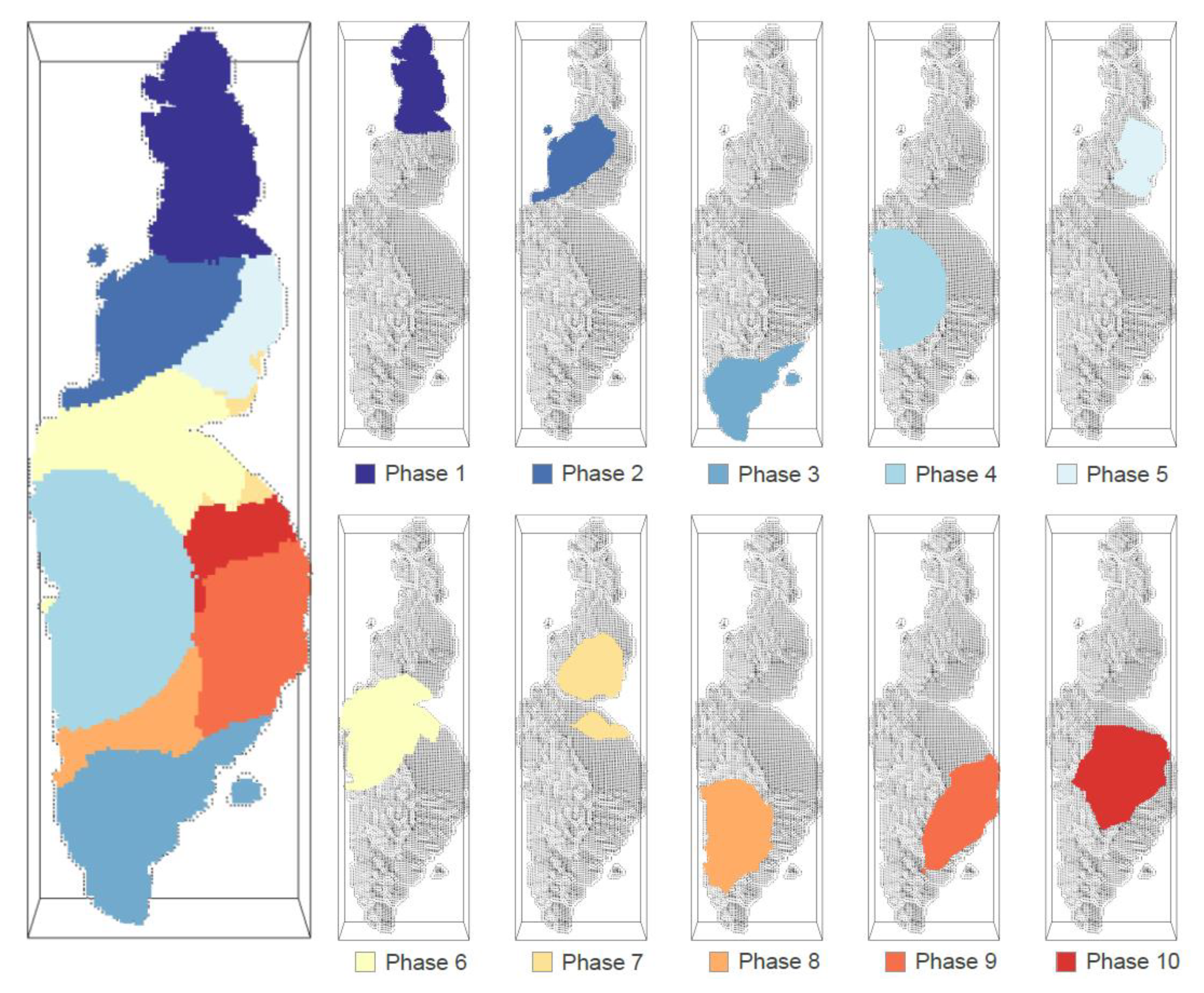
The pushbacks obtained by the algorithm adhere to the typical geometry observed in real-world deposits. Figure 5 illustrates the solution found for the McLaughlin limit mine. On the left side, all increment phases are depicted in the plant view, while on the right, they are individually plotted. The initial increment phases (1 to 5) are assigned to cover the surface, and the final phases (6 to 10) address the deeper regions of the deposit. Increment phase 1 marks the starting point of mining exploitation, and increment phase 7 relies on the exploitation of phases 5 and 6. This precedence is also seen in increment phases 8 and 10, contingent on phases 3 and, 4 and 9.
The clustering algorithm generates subgroups of blocks based on their three-dimensional distance. To do this, all the blocks obtained from the chromosome are used to generate a specific number of clusters defined by the MeanShift algorithm. Figure 6 displays the clusters of the McLaughlin limit mine. The enclosed phases, resulting from the clustering, are visible on the graph’s left side. Meanwhile, the images on the right side reveal the spatial distribution of the solution. This outcome suggests that since the PGA explores positions within the entire grid (as outlined by the parallelepiped in the figure), certain phases might encompass areas without intersecting with the instance’s values. Additionally, Figure 6 highlights that the earlier phases take precedence over those later.
4.6. Production Scheduling
Even though the focus of the algorithm is determining the pushback, in this section, we explore the solution found by the PGA by analyzing the production schedule that is reported by the algorithm. This solution corresponds to the schedule obtained using Algorithm 1, which mimics the best-case method that is known in commercial applications. It is important to emphasize that the PGA uses Algorithm 1 as an approximation of the best possible NPV and that it is relatively fast to compute considering that it is evaluated many times within the genetic algorithm. Therefore, it is not expected to be the best possible schedule.
The solution returned by the algorithm exhibits an average grade that remains consistent across different periods. This uniformity in the tonnage-grade relation reflects an expected homogeneity in the extracted and processed orebody throughout the mine’s life. The grade for a given period is determined based on the extracted tonnage, and these values are then allocated to either mining or processing. The average grade can be calculated for each period from the processed blocks. In examining nine different mines, the extracted tonnage may fluctuate between periods, but the average grade remains comparable. Figure 7 illustrates the tonnage-grade ratio for the KD instance derived from the best schedule found. This graph portrays the total, processed tonnage, and average copper grade over 17 periods. Each bar’s lower portion represents the processed tonnage, while the upper part comprises the remaining blocks. In the 3rd and 11th periods, the processing nears plant capacity, but the plant capacity is underutilized during the other periods.
It is worth emphasizing that the production plan is not fully operational as there are significant variations of the ore and waste tonnage across the scheduled periods. This is expected to from the fact that the production plan is obtained using the best case algorithm, as a way to estimate the NPV of a pushback selection during the execution of the GA. A more realistic production schedule can be obtained afterwards, by using a production scheduling method (for example, applying PCPSP with additional constraints to respect the designed pushbacks).
5. Conclusions
This research presented a novel approach to the problem of optimizing the pushbacks in an open-pit mine, a crucial issue in open-pit mining design. By employing the geometric concept of truncated cones and stepwise extraction, the study unveiled an inventive variation to the pre-existing models. This approach acknowledged ore distribution’s innate complexity and inhomogeneity and successfully incorporated the real-world considerations of extraction and processing capacities on a parallel genetic algorithm. The PGA operates by utilizing a master computer networked to multiple auxiliary systems, which concurrently evaluate the objective function. The selection, crossover, and mutation procedures are carried out on the main thread, while new solutions are evaluated across a series of threads.
This study’s experiments and in-depth analysis lead to some significant conclusions. Firstly, the fine-tuning of parameters using IRACE proved effective, with the three distinct sets of parameters, P1, P2, and P3, demonstrating a significant impact on the PGA performance. Although there were variations among these sets, these did not lead to significant differences in solution quality and computational time, emphasizing the robustness of the PGA model. Also, the radial base and slope angle parameter combination maximized profitability in truncated cone generation. In particular, the parameter combination = (2, 1) offered superior solution quality, consistently achieving the lowest or zero gap percentages, although it required higher computational resources.
Further observations revealed that, while efficient, the PGA could not find values near the ideal or optimal solution, as illustrated by the UPIT. However, considering each mining instance’s complexities and inherent constraints, the PGA generally performed commendably, finding profitable solutions within acceptable computational times. Thus, although the computational time may initially seem high, it is practical in the mining industry context. The planning period of mining operations often spans several years, if not decades, making optimizing these plans a valuable endeavor. Improved efficiency and increased profitability over such extended timelines more than justify the computational time spent. In summary, the PGA has shown its potential as a robust and practical tool for mine planning, offering a promising avenue for future research and applications in the mining industry.
The findings of our current study, while providing valuable insights into the domain of mining optimization, remain constrained to the scenarios of the analyzed mines. Extending these results to mines with more extensive mining operations would be conjectural, considering the complex and distinct challenges such operations entail. Moreover, the study predominantly focused on singular objectives, leaving a considerable void in understanding how simultaneous multiple objectives would influence computational performance. Multi-objective scenarios often mirror real-world complexities, and understanding them can offer a more holistic view of mining optimization. Hence, future studies might explore these concerns in depth.
Author Contributions
Methodology, F.N., N.M., C.C.-B., C.R. and V.P.; Validation, F.N., N.M., C.C.-B., C.R. and V.P.; Formal analysis, F.N., N.M., C.C.-B., C.R. and V.P.; Investigation, F.N., N.M., C.C.-B., C.R. and V.P.; Writing—original draft, F.N., N.M., C.C.-B., C.R. and V.P.; Writing—review & editing, F.N., N.M., C.C.-B., C.R. and V.P. All authors have read and agreed to the published version of the manuscript.
Funding
This work was funded by the ANID PIA /BASAL AFB220002 and AFB230001, USACH Sabbatical Project VP-2022-2023, USA1899-Vridei 061919VP-PAP Universidad de Santiago de Chile, and DICYT- USACH 061919PD. Also, by the National Agency for Research and Development (ANID)/Scholarship Program/Doctorado Becas Chile/2018-72190600 and Subvención a la Instalación en la Academia, Folio 85220108. Finally, the work is also funded by Vicerrectoria de Investigación y Postgrado (VRIP) through the “Proyecto de Investigación Interno 2023”: RE2360219. This project is also funded by CONICYT PIA/BASAL: AFB230001-ANID.
Data Availability Statement
Data sharing does not apply to this article as no new data were created in this study.
Acknowledgments
The authors are grateful to the ALGES laboratory for their support in providing computational resources for running the experiments.
Conflicts of Interest
The authors declare no conflicts of interest.
References
- Hustrulid, W.; Kuchta, M. Open Pit Mine Planning and Design. Volume 1—Fundamentals; U.S. Department of Energy Office of Scientific and Technical Information: Oak Ridge, TN, USA, 1995. [Google Scholar]
- Lambert, W.B.; Newman, A.M. Tailored Lagrangian Relaxation for the Open Pit Block Sequencing Problem. Ann. Oper Res. 2014, 222, 419–438. [Google Scholar] [CrossRef]
- Lerchs, H.; Grossman, F. Optimum Design of Open-Pit Mines. Transaction. CIM 1965, 47–54. [Google Scholar]
- Hochbaum, D.S. A New—Old Algorithm for Minimum-Cut and Maximum-Flow in Closure Graphs. Networks 2001, 37, 171–193. [Google Scholar] [CrossRef]
- Chicoisne, R.; Espinoza, D.; Goycoolea, M.; Moreno, E.; Rubio, E. A New Algorithm for the Open-Pit Mine Production Scheduling Problem. Oper. Res. 2012, 60, 517–528. [Google Scholar] [CrossRef]
- Espinoza, D.; Goycoolea, M.; Moreno, E.; Newman, A. MineLib: A Library of Open Pit Mining Problems. Ann. Oper Res. 2013, 206, 93–114. [Google Scholar] [CrossRef]
- Nancel-Penard, P.; Morales, N.; Cornillier, F. A Recursive Time Aggregation-Disaggregation Heuristic for the Multidimensional and Multiperiod Precedence-Constrained Knapsack Problem: An Application to the Open-Pit Mine Block Sequencing Problem. Eur. J. Oper. Res. 2022, 303, 1088–1099. [Google Scholar] [CrossRef]
- Whittle, D.; Whittle, J.; Wharton, C.; Hall, G. Strategic Mine Planning; Gemcom Software International Inc.: Melbourne, Australia, 2005. [Google Scholar]
- Bai, X.; Marcotte, D.; Gamache, M.; Gregory, D.; Lapworth, A. Automatic Generation of Feasible Mining Pushbacks for Open Pit Strategic Planning. J. S. Afr. Inst. Min. Metall. 2018, 118, 514–530. [Google Scholar] [CrossRef]
- Tabesh, M.; Mieth, C.; Askari–Nasab, H. A Multi–Step Approach to Long–Term Open–Pit Production Planning. Int. J. Min. Miner. Eng. 2014, 5, 273–298. [Google Scholar] [CrossRef]
- Morales, N.; Nelis, G.; Amaya, J. An Efficient Method for Optimizing Nested Open Pits with Operational Bottom Space. Int. Trans. Oper. Res. 2023. [Google Scholar] [CrossRef]
- Jélvez, E.; Morales, N.; Nancel-Penard, P.; Peypouquet, J.; Reyes, P. Aggregation Heuristic for the Open-Pit Block Scheduling Problem. Eur. J. Oper. Res. 2016, 249, 1169–1177. [Google Scholar] [CrossRef]
- Liu, S.Q.; Kozan, E. New Graph-Based Algorithms to Efficiently Solve Large Scale Open Pit Mining Optimisation Problems. Expert Syst. Appl. 2016, 43, 59–65. [Google Scholar] [CrossRef]
- Cullenbine, C.; Wood, R.K.; Newman, A. A Sliding Time Window Heuristic for Open Pit Mine Block Sequencing. Optim. Lett. 2011, 5, 365–377. [Google Scholar] [CrossRef]
- Vossen, T.W.M.; Wood, R.K.; Newman, A.M. Hierarchical Benders Decomposition for Open-Pit Mine Block Sequencing. Oper. Res. 2016, 64, 771–793. [Google Scholar] [CrossRef]
- Samavati, M.; Essam, D.; Nehring, M.; Sarker, R. A Local Branching Heuristic for the Open Pit Mine Production Scheduling Problem. Eur. J. Oper. Res. 2017, 257, 261–271. [Google Scholar] [CrossRef]
- Eiben, A.E.; Smith, J.E. Introduction to Evolutionary Computing; Natural Computing Series; Springer: Berlin, Heidelberg, 2015; ISBN 978-3-662-44873-1. [Google Scholar]
- Talbi, E.-G. Metaheuristics: From Design to Implementation; John Wiley & Sons: Hoboken, NJ, USA, 2009; ISBN 978-0-470-49690-9. [Google Scholar]
- Elsayed, S.; Sarker, R.; Essam, D.; Coello Coello, C.A. Evolutionary Approach for Large-Scale Mine Scheduling. Inf. Sci. 2020, 523, 77–90. [Google Scholar] [CrossRef]
- Denby, B.; Schofield, D.; Hunter, G. Genetic Algorithms for Open Pit Schedulingextension into 3-Dimensions. In Proceedings of the Proceedings 5th International Symposium on Mine Planning and Equipment Selection, Sao Paulo, Brazil, 22–25 October 1996. [Google Scholar]
- Myburgh, C.; Deb, K. Evolutionary Algorithms in Large-Scale Open Pit Mine Scheduling. In Proceedings of the 12th Annual Conference on Genetic and Evolutionary Computation, Portland, OR, USA, 7–11 July 2010; Association for Computing Machinery: New York, NY, USA, 2010; pp. 1155–1162. [Google Scholar]
- Milani, G. A Genetic Algorithm with Zooming for the Determination of the Optimal Open Pit Mines Layout. Open Civ. Eng. J. 2016, 10. [Google Scholar] [CrossRef]
- Alipour, A.; Khodaiari, A.A.; Jafari, A.; Tavakkoli-Moghaddam, R. Production Scheduling of Open-Pit Mines Using Genetic Algorithm: A Case Study. Int. J. Manag. Sci. Eng. Manag. 2020, 15, 176–183. [Google Scholar] [CrossRef]
- Azadi, N.; Mirzaei-Nasirabad, H.; Mousavi, A. A Genetic Algorithm Scheme for Large Scale Open-Pit Mine Production Scheduling. Min. Technol. 2023, 132, 225–236. [Google Scholar] [CrossRef]
- Ferland, J.A.; Amaya, J.; Djuimo, M.S. Application of a Particle Swarm Algorithm to the Capacitated Open Pit Mining Problem. In Autonomous Robots and Agents; Mukhopadhyay, S.C., Gupta, G.S., Eds.; Studies in Computational Intelligence; Springer: Berlin, Heidelberg, 2007; pp. 127–133. ISBN 978-3-540-73424-6. [Google Scholar]
- Khan, A.; Niemann-Delius, C. Production Scheduling of Open Pit Mines Using Particle Swarm Optimization Algorithm. Adv. Oper. Res. 2014, 2014, e208502. [Google Scholar] [CrossRef]
- Wharton, C.; Whittle, J. The Effect of Minimum Mining Width on NPV. Optim. Whittle 1997, 173–178. [Google Scholar]
- Nancel-Penard, P.; Morales, N. Optimizing Pushback Design Considering Minimum Mining Width for Open Pit Strategic Planning. Eng. Optim. 2022, 54, 1494–1508. [Google Scholar] [CrossRef]
- Goldberg, D.E. Genetic Algorithms in Search, Optimization and Machine Learning, 1st ed.; Addison-Wesley Longman Publishing Co., Inc.: San Francisco, CA, USA, 1989; ISBN 978-0-201-15767-3. [Google Scholar]
- Rothlauf, F. Representations for Genetic and Evolutionary Algorithms. In Representations for Genetic and Evolutionary Algorithms; Rothlauf, F., Ed.; Springer: Berlin, Heidelberg, 2006; pp. 9–32. ISBN 978-3-540-32444-7. [Google Scholar]
- Comaniciu, D.; Meer, P. Mean Shift: A Robust Approach toward Feature Space Analysis. IEEE Trans. Pattern Anal. Mach. Intell. 2002, 24, 603–619. [Google Scholar] [CrossRef]
- Scikit-Learn: Machine Learning in Python—Scikit-Learn 1.3.2 Documentation. Available online: https://scikit-learn.org/stable/ (accessed on 23 December 2023).
- López-Ibáñez, M.; Dubois-Lacoste, J.; Pérez Cáceres, L.; Birattari, M.; Stützle, T. The Irace Package: Iterated Racing for Automatic Algorithm Configuration. Oper. Res. Perspect. 2016, 3, 43–58. [Google Scholar] [CrossRef]
Figure 1.
Representation of a truncated cone.

Figure 2.
Representation of an individual of the PGA. (a) The individual is composed of four centers, each including other centers circumscribed by the radius , i.e., the center 46 includes the centers 36, 45, 47, and 56. (b) The individual’s genotype, after the clustering process considers only the centers, in this case, three clusters are formed with colors gray, blue and green.

Figure 3.
Steps to evaluate the NPV fitness function.

Figure 4.
PGA operators. (a) Crossover operator h1 is composed of the intersection of p1 and p2, while h2 arises from their symmetric difference. (b) Mutation, an element of p1, is dropped as the set differences between p1 and the element {3}.
Figure 4.
PGA operators. (a) Crossover operator h1 is composed of the intersection of p1 and p2, while h2 arises from their symmetric difference. (b) Mutation, an element of p1, is dropped as the set differences between p1 and the element {3}.

Figure 5.
Extraction phases (highlighted by color) for the McLaughlin limit instance.

Figure 6.
Clustering in the McLaughlin limit instance. Each cluster is represented by a different color.
Figure 6.
Clustering in the McLaughlin limit instance. Each cluster is represented by a different color.

Figure 7.
Example of the production plan used to estimate the fitness of the pushback selection for the KD instance.
Figure 7.
Example of the production plan used to estimate the fitness of the pushback selection for the KD instance.


Table 1.
Set of instances for CPIT.
| Name | Number of Blocks | Number of Precedences | CM (t) | CP1 (t) | CP2 (t) | |
|---|---|---|---|---|---|---|
| Newman1 | 1060 | 3922 | 2,000,000 | 1,100,000 | 0.08 | |
| Zuck small | 9400 | 145,640 | 60,000,000 | 20,000,000 | 0.10 | |
| KD | 14,153 | 219,778 | - | 10,000,000 | 0.15 | |
| Zuck medium | 29,277 | 1,271,207 | 18,000,000 | 8,000,000 | 0.10 | |
| P4HD | 40,947 | 738,609 | 52,500,000 | 12,500,000 | 0.15 | |
| Marvin | 53,271 | 650,631 | 60,000,000 | 20,500,000 | 0.10 | |
| W23 | 74,260 | 764,786 | 68,000,000 | 3,610,000 | 1,000,000 | 0.10 |
| Zuck large | 96,821 | 1,053,105 | 3,000,000 | 1,200,000 | 0.10 | |
| McLaughlin limit | 112,687 | 3,035,483 | 3,000,000 | - | - | 0.15 |
Table 2.
Set of parameters for the PGA.
| Set | # Nch | # Ngen | # Npop | Cx |
|---|---|---|---|---|
| P1 | 15 | 10 | 50 | 0.7 |
| P2 | 10 | 10 | 50 | 0.8 |
| P3 | 15 | 10 | 50 | 0.9 |
Table 3.
Solution quality (gap) and computer time (seconds).
| Instance | (r, δ) = (1, 1) | (r, δ) = (1,2) | (r, δ) = (2, 1) | (r, δ) = (2, 2) | ||||
|---|---|---|---|---|---|---|---|---|
| P1 | P1 | P1 | Set 1 | |||||
| %Gap | Time [s] | %Gap | Time [s] | %Gap | Time [s] | %Gap | Time [s] | |
| Newman1 | 0.670 | 5.99 | 1.120 | 9.76 | 0.000 | 6.48 | 1.170 | 9.92 |
| Zuck_small | 9.290 | 38.73 | 10.150 | 61.21 | 0.190 | 205.70 | 0.000 | 203.08 |
| KD | 38.140 | 74.66 | 24.260 | 121.69 | 0.000 | 281.69 | 1.410 | 201.92 |
| Zuck_medium | 2.070 | 1740.19 | 14.650 | 1706.75 | 0.000 | 7252.18 | 3.860 | 8173.29 |
| Average | 12.540 | 464.89 | 12.540 | 474.85 | 0.050 | 1936.51 | 1.610 | 2147.05 |
| P2 | P2 | P2 | Set 2 | |||||
| %Gap | Time [s] | %Gap | Time [s] | %Gap | Time [s] | %Gap | Time [s] | |
| Newman1 | 1.910 | 5.34 | 2.370 | 8.36 | 0.000 | 5.79 | 0.690 | 8.60 |
| Zuck_small | 15.580 | 35.64 | 10.130 | 55.64 | 0.190 | 196.16 | 0.000 | 188.01 |
| KD | 39.670 | 68.87 | 24.460 | 110.40 | 0.000 | 249.51 | 1.100 | 195.82 |
| Zuck_medium | 2.060 | 1572.44 | 14.230 | 1575.65 | 0.000 | 6527.97 | 2.830 | 7092.59 |
| Average | 14.800 | 420.57 | 12.800 | 437.51 | 0.050 | 1744.86 | 1.150 | 1871.25 |
| P3 | P3 | P3 | Set 3 | |||||
| %Gap | Time [s] | %Gap | Time [s] | %Gap | Time [s] | %Gap | Time [s] | |
| Newman1 | 1.860 | 5.71 | 1.940 | 9.08 | 0.000 | 6.16 | 1.070 | 9.13 |
| Zuck_small | 16.360 | 37.29 | 10.600 | 58.19 | 0.860 | 187.88 | 0.000 | 192.62 |
| KD | 40.110 | 72.19 | 24.690 | 114.50 | 0.000 | 245.88 | 2.180 | 193.09 |
| Zuck_medium | 4.070 | 1625.08 | 17.150 | 1714.45 | 0.000 | 7076.19 | 6.600 | 7380.23 |
| Average | 15.600 | 435.07 | 13.600 | 474.06 | 0.210 | 1879.03 | 2.470 | 1943.77 |
Table 4.
Results for large-size instances.
| Mine Instance | UPIT (NPV) | PGA; (r, δ) = (2, 1) | |||
|---|---|---|---|---|---|
| Best Profit (NPV) | Average Profit (NPV) | Average # Periods | Average Computer Time [s] | ||
| P4HD | 293,373,256.00 | 170,741,330.74 | 167,048,191.44 | 7.43 | 9803.98 |
| Marvin | 1,145,655,436.00 | 201,860,355.53 | 103,224,207.28 | 32.14 | 1730.65 |
| W23 | 510,973,998.00 | 210,721,614.33 | 182,753,331.71 | 10.25 | 40,506.99 |
| Zuck large | 122,220,280.00 | 59,989,326.16 | 58,084,976.43 | 18.00 | 11,347.07 |
| McLaughlin limit | 1,495,726,474.00 | 954,741,233.01 | 876,234,136.37 | 8.57 | 30,343.03 |
Disclaimer/Publisher’s Note: The statements, opinions and data contained in all publications are solely those of the individual author(s) and contributor(s) and not of MDPI and/or the editor(s). MDPI and/or the editor(s) disclaim responsibility for any injury to people or property resulting from any ideas, methods, instructions or products referred to in the content. |
© 2024 by the authors. Licensee MDPI, Basel, Switzerland. This article is an open access article distributed under the terms and conditions of the Creative Commons Attribution (CC BY) license (https://creativecommons.org/licenses/by/4.0/).
Share and Cite
MDPI and ACS Style
Navarro, F.; Morales, N.; Contreras-Bolton, C.; Rey, C.; Parada, V. Open-Pit Pushback Optimization by a Parallel Genetic Algorithm. Minerals 2024, 14, 438. https://doi.org/10.3390/min14050438
AMA Style
Navarro F, Morales N, Contreras-Bolton C, Rey C, Parada V. Open-Pit Pushback Optimization by a Parallel Genetic Algorithm. Minerals. 2024; 14(5):438. https://doi.org/10.3390/min14050438
Chicago/Turabian StyleNavarro, Felipe, Nelson Morales, Carlos Contreras-Bolton, Carlos Rey, and Victor Parada. 2024. "Open-Pit Pushback Optimization by a Parallel Genetic Algorithm" Minerals 14, no. 5: 438. https://doi.org/10.3390/min14050438
Note that from the first issue of 2016, this journal uses article numbers instead of page numbers. See further details here.