Grade Distribution Modeling within the Bauxite Seams of the Wachangping Mine, China, Using a Multi-Step Interpolation Algorithm

Abstract

Mineral reserve estimation and mining design depend on a precise modeling of the mineralized deposit. A multi-step interpolation algorithm, including 1D biharmonic spline estimator for interpolating floor altitudes, 2D nearest neighbor, linear, natural neighbor, cubic, biharmonic spline, inverse distance weighted, simple kriging, and ordinary kriging interpolations for grade distribution on the two vertical sections at roadways, and 3D linear interpolation for grade distribution between sections, was proposed to build a 3D grade distribution model of the mineralized seam in a longwall mining panel with a U-shaped layout having two roadways at both sides. Compared to field data from exploratory boreholes, this multi-step interpolation using a natural neighbor method shows an optimal stability and a minimal difference between interpolation and field data. Using this method, the 97,576 m³ of bauxite, in which the mass fraction of Al₂O₃ (W_a) and the mass ratio of Al₂O₃ to SiO₂ (W_a/s) are 61.68% and 27.72, respectively, was delimited from the 189,260 m³ mineralized deposit in the 1102 longwall mining panel in the Wachangping mine, Southwest China. The mean absolute errors, the root mean squared errors and the relative standard deviations of errors between interpolated data and exploratory grade data at six boreholes are 2.544, 2.674, and 32.37% of W_a; and 1.761, 1.974, and 67.37% of W_a/s, respectively. The proposed method can be used for characterizing the grade distribution in a mineralized seam between two roadways at both sides of a longwall mining panel.

1. Introduction

Ore reserve estimations and mining designs of underground mines depend on precise three-dimensional modeling of the mineralized seam for achieving the position coordinate description and the grade distribution of the mineral. Therefore, the grade distribution modeling of the mineralized deposit is a fundamental task [1]. However, the reference data are frequently sparse and scattered, and no data is available from positions between sample points [2]. Hence, it is often necessary to interpolate data values for locations where there are no measurements using statistical and deterministic interpolation methods, and local and global interpolations [3,4,5,6,7,8]. Concerning statistical methods, the kriging-based methods are commonly used by weighting data points for interpolating unknown locations based on their relative distances using a variogram model to evaluate the autocorrelation of spatial data [2,9,10,11]. For deterministic methods, the nearest neighbor, natural neighbor, linear, cubic, spline, and inverse distance weighted methods can be selected [12,13]. In global methods, the interpolation depends on all sample points, while the local interpolation methods depend only on the data in its neighborhood [4]. Additionally, artificial neural networks [14], fuzzy methodology [15,16], evolutionary algorithms [17], support vector machines [18], and fractal models [19] have also been used to estimate the grade of the mineralized deposits.

When the sample points have a regular distribution, for example on a rectangular mesh grid, many methods are available for continuous and smooth interpolation [20]. However, for underground mineral seams, the occurrence conditions often result in the obviously irregular distributions of sample points and the high scale differences in three dimensions. The methods mentioned above are less satisfactory in depicting the thin and anfractuous stratiform deposit, and it is difficult to achieve a smooth and exact interpolation from exceedingly irregular distributions and large variations of sample data.

In this paper, a multi-step interpolation algorithm—including one-dimensional (1D) biharmonic spline interpolation for interpolating floor altitudes, two-dimensional (2D) interpolation for grade distribution on the two vertical sections, and three-dimensional (3D) linear interpolation for grade distribution between sections—was proposed to build a 3D grade distribution model for the mineralized seam in a longwall mining panel with U-shaped layout, in which the two roadways at both sides of the panel were prepared before mining to perform the ventilation and transportation. For the 1102 panel in the Wachangping bauxite mine, the irregular sampling data with large variations in the strike-altitude coordinate frame, measured in the two roadways on both sides of the panel, were mapped into a regular rectangular mesh grid in the strike-height coordinate frame by subtracting floor altitudes at sampling locations from corresponding sampling altitudes. Then the conventional methods—such as the nearest neighbor, linear, natural neighbor, cubic, and biharmonic spline, inverse distance weighted, and kriging-based interpolations—are used for smooth and exact interpolations. Subsequently, the interpolated floor altitudes of roadways were used to recover the interpolation data in the strike-height coordinate frame into the strike-altitude coordinate frame by adding the interpolated floor altitudes and the mapped heights at interpolation locations together. Finally, the grade values between roadways were estimated by 3D linear interpolation and confirmed by field data from exploratory boreholes. The proposed method is applicable to estimate the grade distribution in a mineralized seam in which a longwall mining panel with U-shaped layout is used to perform the mining operations.

2. Methodology

For underground mineral seams, an accurate orebody model—including its position and grade data—is a necessary precondition for conducting a mining plan to achieve low dilution and high recovery of mineral resources. Longwall mining technology, a widely-used method for mechanized continuous and large-scale extraction of underground coal [21,22,23,24,25,26], was progressively introduced for extracting an underground mineral seam, for example, a bauxite seam [27,28]. In the longwall mining panel, in general, the two roadways at both sides of the panel, called the tail roadway and the head roadway, are excavated to provide ventilation and transportation for mining operations. The mineral composition of ore samples excavated from roadway walls can be measured to assess the grade of the mineralized seam. The key steps of the multi-step interpolation for quantifying the grade distribution of the mineralized seam are depicted in Figure 1.

It can be seen from Figure 1 that the 3D grade distribution model of the mineral seam can be established by the five-step interpolation process, which is shown as follows:

Firstly, according to the 2D function-based interpolation methods, the mineral grade distribution on the tail roadway wall relative to floor can be given by Equation (1).

$$g_{\mathrm{t}}(x,h)=f_{2-\mathrm{D}}^{\mathrm{t}}(x,h)$$

(1)

where $g_{\mathrm{t}}(x,h)$ is the grade distribution on the tail roadway wall relative to the floor, h is the vertical height of a position from the roadway floor, and $f_{2-\mathrm{D}}^{\mathrm{t}}$ is a 2D interpolation function determined by the scattered sample points $(x_i,h_i,g_{\mathrm{t}i})$ on the tail roadway wall, which involves not only the triangulation-based interpolation methods including nearest neighbor, linear, natural neighbor, or cubic interpolations, but also the biharmonic spline interpolation method [29].

The inverse distance weighted (IDW) interpolation can be also used to estimate the mineral grade distribution on the tail roadway wall relative to floor, which uses the following Equations (2) and (3).

$$g_{\mathrm{t}}(x,h)={\displaystyle \sum _{i=1}^{N_S}(d_{S_i}^{-u}/{\displaystyle {\sum }_i^{N_S}{d}_{S_i}^{-u}})}\cdot g_{\mathrm{t}i}$$

(2)

$$d_{S_i}=\sqrt{{(x-x_i)}^2+{(h-h_i)}^2}$$

(3)

where $N_S$ is the number of sample points, $d_{S_i}$ is the distance between the ith sample point and the interpolated point [30].

In statistical methods, we also utilized the simple kriging (SK) and ordinary kriging (OK) interpolations, which are the most widely used kriging-based methods, to achieve the grade distribution on the roadway wall. A semivariogram shown as Equation (4) is calculated to quantify the spatial correlation between a point and its surrounding points within a particular distance. The conventional kriging estimator is shown in Equation (5), in which the kriging weight is based on minimizing the variance of the form Equation (6).

$${\gamma }_e(d)=\frac{1}{2n}{\displaystyle \sum _{i=1}^n{\left[g_{\mathrm{t}i}(x_i)-g_{\mathrm{t}i}(x_i+d)\right]}^2}$$

(4)

$$g_{\mathrm{t}}(x)={\displaystyle \sum _{i=1}^{N_S}{\lambda }_i}\cdot g_{\mathrm{t}i}(x_i)$$

(5)

$${\sigma }^2={\displaystyle \sum _{i=1}^{N_S}{\lambda }_i}\cdot {\gamma }_f(x_i,x)+\mu$$

(6)

where n is the number of pairs of observations separated by distance d, ${\gamma }_e(d)$ is the experimental variogram obtained by changing d, ${\lambda }_i$ is the kriging weight for interpolating the ith point with ${\displaystyle {\sum }_i^{N_S}{\lambda }_i}=1$, ${\sigma }^2$ is the kriging interpolation variance, and the μ is the Lagrange multiplier which is required for the minimization [31].

Secondly, based on the 1D biharmonic spline interpolation, the floor altitude of the tail roadway can be expressed by Equation (7) [32].

$$z_{\mathrm{b}}^{\mathrm{t}}(x)={\displaystyle \sum _{j=1}^M{k}_j^{\mathrm{t}}}{\left|x-x_j\right|}^3$$

(7)

where $z_{\mathrm{b}}^{\mathrm{t}}$ is the floor altitude of the tail roadway, and $k_j^{\mathrm{t}}$ is the 1D biharmonic spline interpolation coefficient solved by the following linear system expressed by Equation (8).

$$z_{\mathrm{b}}^{\mathrm{t}}(x_i)={\displaystyle \sum _{j=1}^M{k}_j^{\mathrm{t}}}{\left|x_i-x_j\right|}^3$$

(8)

where $(x_i,z_{\mathrm{b}}^{\mathrm{t}}(x_i))$ is the position of a sampling point from M scattered sampling points on the tail roadway wall.

Thirdly, similar to Step 1, the grade distribution on the head roadway wall relative to floor, $g_{\mathrm{h}}(x,h)$, can be obtained according to the above interpolation methods determined by the scattered sampling points, $(x_i,h_i,g_{\mathrm{h}i})$, on the head roadway wall.

Fourthly, according to the 1D biharmonic spline interpolation algorithm, the floor altitude of head roadway can be expressed by Equation (9).

$$z_{\mathrm{b}}^{\mathrm{h}}(x)={\displaystyle \sum _{j=1}^N{k}_j^{\mathrm{h}}}{\left|x-x_j\right|}^3$$

(9)

where $z_{\mathrm{b}}^{\mathrm{h}}$ is the floor altitude of the head roadway, and $k_j^{\mathrm{h}}$ is the 1D biharmonic spline interpolation coefficient solved by the following linear system show in Equation (10).

$$z_{\mathrm{b}}^{\mathrm{h}}(x_i)={\displaystyle \sum _{j=1}^N{k}_j^{\mathrm{h}}}{\left|x_i-x_j\right|}^3$$

(10)

where $(x_i,z_{\mathrm{b}}^{\mathrm{h}}(x_i))$ is the position of a sampling point from N scattered sampling points on the head roadway wall.

Finally, the grade distribution on the tail and head roadway walls can be represented as Equations (11) and (12), respectively.

$$\{\begin{array}{l}{g}_{\mathrm{t}}(x_{\mathrm{t}},z_{\mathrm{t}})=g_{\mathrm{t}}(x_{\mathrm{t}},h_{\mathrm{t}})\\ z_{\mathrm{t}}=z_{\mathrm{b}}^{\mathrm{t}}+h_{\mathrm{t}}\end{array}$$

(11)

$$\{\begin{array}{l}{g}_{\mathrm{h}}(x_{\mathrm{h}},z_{\mathrm{h}})=g_{\mathrm{h}}(x_{\mathrm{h}},h_{\mathrm{h}})\\ z_{\mathrm{h}}=z_{\mathrm{b}}^{\mathrm{h}}+h{}_{\mathrm{h}}\end{array}$$

(12)

The grade distribution between roadways can be achieved by the 3D linear interpolation algorithm, which is given by Equation (13).

$$\{\begin{array}{l}g(x,y,z)=g_{\mathrm{t}}(x_{\mathrm{t}},z_{\mathrm{t}})+\frac{y-y_{\mathrm{t}}}{y_{\mathrm{h}}-y_{\mathrm{t}}}\left[g_{\mathrm{h}}(x_{\mathrm{h}},z_{\mathrm{h}})-g_{\mathrm{t}}(x_{\mathrm{t}},z_{\mathrm{t}})\right]\\ x=x_{\mathrm{t}}+\frac{y-y_{\mathrm{t}}}{y_{\mathrm{h}}-y_{\mathrm{t}}}(x_{\mathrm{h}}-x_{\mathrm{t}})\\ z=z_{\mathrm{t}}+\frac{y-y_{\mathrm{t}}}{y_{\mathrm{h}}-y_{\mathrm{t}}}(z_{\mathrm{h}}-z_{\mathrm{t}})\end{array}$$

(13)

where $g(x,y,z)$, $g_{\mathrm{t}}(x_{\mathrm{t}},z_{\mathrm{t}})$, and $g_{\mathrm{h}}(x_{\mathrm{h}},z_{\mathrm{h}})$ are the grade distributions between roadways, on the tail roadway wall, and on the head roadway wall, respectively; and $(x_{\mathrm{t}},y_{\mathrm{t}},z_{\mathrm{t}})$ and $(x_{\mathrm{h}},y_{\mathrm{h}},z_{\mathrm{h}})$ are a pair of positions on the tail and head roadway walls shown as black dots in Figure 1e, respectively.

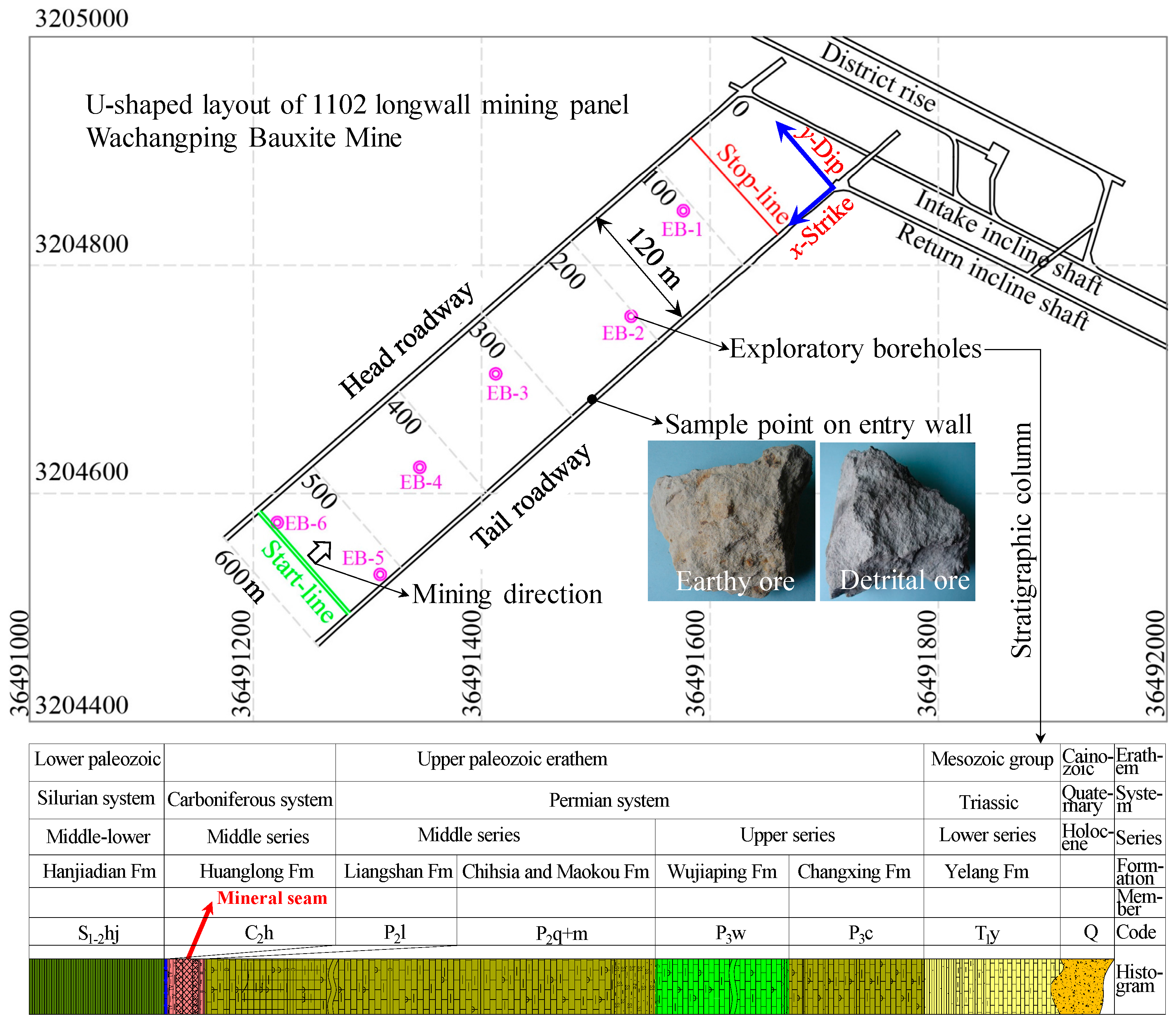
3. Scattered Grade Data

The above interpolation method is applied to interpolate the grade distribution in the bauxite seams of the Wachangping bauxite mine (China). The 1102 longwall panel is 500 m in length (from the stop-line of mining at x = 59.501 to the start-line at x = 559.501) and 120 m in width (from the tail roadway at y = 0 to the head roadway y = 120) in the Wachangping bauxite mine, as shown in Figure 2. The mineral composition of the bauxite ore or bauxitic rock was measured in 53 groups of ore samples excavated from the roadway walls, which include 27 groups from the tail roadway and 26 groups from the head roadway. The mass fraction of Al₂O₃ and SiO₂ are achieved and depicted in Figure 3.

4. Grade Distribution Model

Using the scattered sampling data measured from the roadway walls, the multi-step interpolation algorithm was proposed to establish a 3D grade distribution model of the mineralized seam, based on the coupled interpolation method comprising of the 2D nearest neighbor, linear, natural neighbor, cubic, biharmonic spline; IDW, SK, or OK, 1D biharmonic spline; and 3D linear interpolations. As the examples show, the grade distribution at the cross-sections of y = 0, 20, 40, 60, 80, 100, and 120 m in the mineralized seams are shown in Figure 4. The grade values are expressed by the two indices, namely the mass fraction of Al₂O₃ marked as W_a and the mass ratio of Al₂O₃ to SiO₂ marked as W_a/s. Corresponding to the 2D nearest neighbor, linear, natural neighbor, cubic, biharmonic spline, IDW, SK, and OK interpolation methods adopted in the interpolating processes for grade distributions on roadway walls relative to floors, the slice maps of the grade distributions are shown in Figure 4a–h, respectively. It is evident that the bauxite seam presents a distinct stratiform structure, because it belongs to a sedimentary mineral deposit embedded in the sedimentary strata.

Since bauxite is subjected to the development levels of mineral processing and metallurgy in the bauxite/aluminium industry, the grade of bauxite should satisfy certain Chinese industrial constraints, which require that the minimum W_a and W_a/s in the bauxite seam are 55% and 3.5, respectively [33]. The slice maps of the orebody delimited by the above indices are shown in Figure 5.

5. Results and Discussion

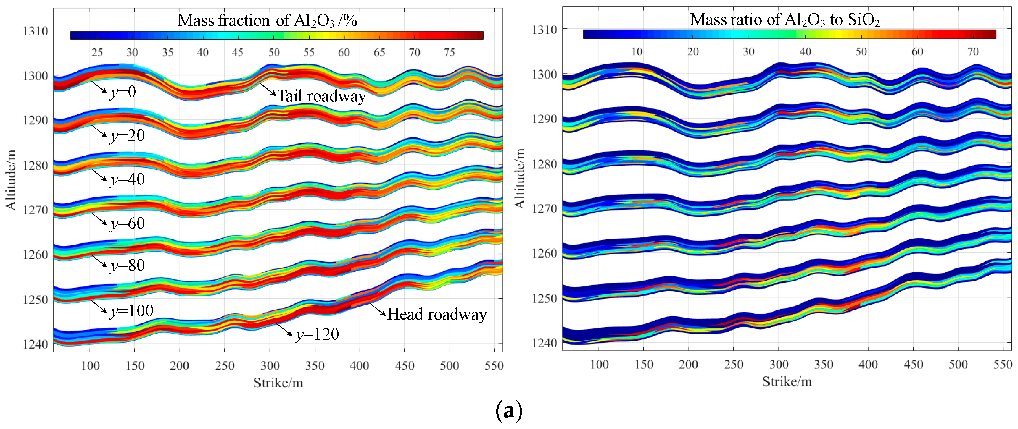
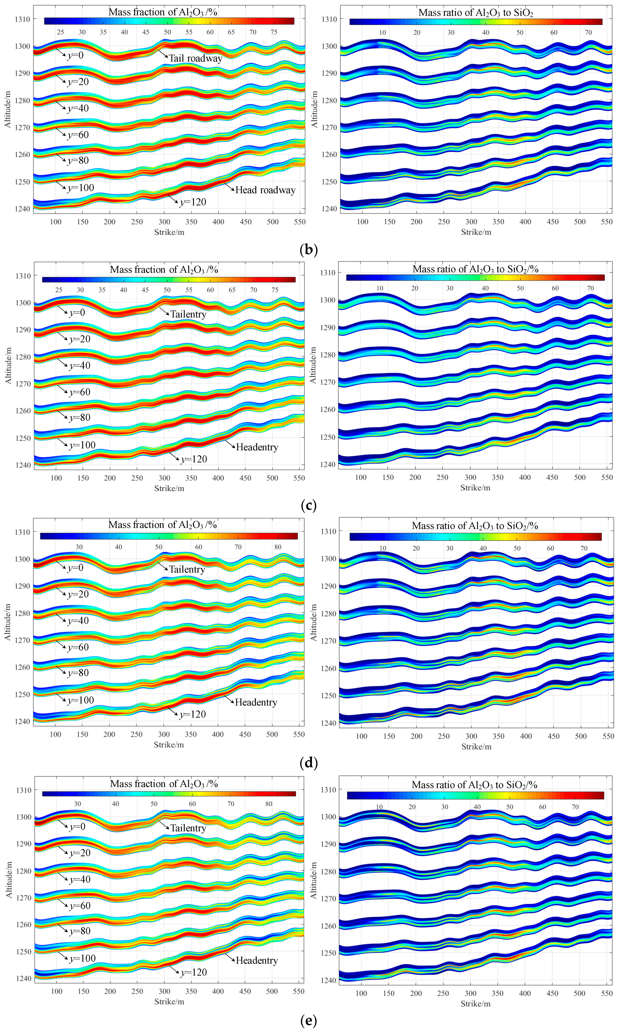
5.1. Comparison of Interpolation Methods

According to the bauxite grade distribution models established by the multi-step interpolation algorithm in which the 2D nearest neighbor, linear, natural neighbor, cubic, biharmonic spline, IDW, SK, and OK interpolation methods are used in the interpolation processes for grade distribution on the roadway walls, some characteristic and comparative indices can be calculated, which are listed in

Table 1. Comparative data of the different interpolation methods.

Method	Bauxite Seam Volume/m3	Ore Reserve/m3	In-Situ Average Grade of Bauxite Seam ${\mathit{G}}_{\mathit{S}}=\frac{1}{{\mathit{N}}_{\mathit{S}}}{\displaystyle \sum _{\mathit{i}=1}^{{\mathit{N}}_{\mathit{S}}}{\mathit{G}}_{\mathit{S}\mathit{i}}}$		Average Grade of Bauxite Orebody Applying Industrial Constrains ${\mathit{G}}_{\mathit{O}}=\frac{1}{{\mathit{N}}_{\mathit{O}}}{\displaystyle \sum _{\mathit{i}=1}^{{\mathit{N}}_{\mathit{O}}}{\mathit{G}}_{\mathit{O}\mathit{i}}}$		Assessment of Difference Ratio Between Interpolation Data and Sample Data Dis/%						Time Consuming/s
			Wa/% (SD)	Wa/s (SD)	Wa/% (SD)	Wa/s (SD)	Mean		Max		Min
							Wa	Wa/s	Wa	Wa/s	Wa	Wa/s
Nearest	189,260	97,750	54.80 (15.53)	17.89 (18.94)	63.73 (7.54)	29.20 (17.18)	18.48	45.24	0	0	0	0	76.2
Linear	189,260	96,192	54.84 (13.28)	17.52 (14.98)	61.78 (7.08)	27.18 (11.84)	18.58	42.19	−0.12	0	0	0.09	80.4
Natural	189,260	97,576	54.88 (13.11)	18.02 (14.48)	61.68 (6.85)	27.72 (10.27)	17.67	35.92	−0.15	0	0	0.09	81.4
Cubic	189,260	98,151	55.32 (13.82)	17.57 (16.01)	62.34 (7.59)	27.30 (13.34)	19.6	42.67	6.44	1.74	−4.34	−50.9	76.2
Biharmonic	189,260	99,763	56.32 (13.94)	17.38 (16.59)	62.78 (7.97)	26.97 (14.59)	21.76	41.14	9.03	6.59	−1.41	−51.4	78.1
IDW	189,260	93,348	53.15 (12.93)	17.40 (14.31)	60.74 (6.17)	27.44 (10.79)	14.92	41.27	0	0	0.05	0	153.3
SK	189,260	100,750	55.34 (14.11)	18.28 (15.87)	62.88 (7.19)	28.52 (11.77)	19.65	48.37	2.21	0	0	−58.3	2161.7
			[E: 11.22]	[E: 11.71]
			[EV: 2.04]	[EV: 0.97]
OK	189,260	100,630	55.28 (14.12)	18.24 (15.89)	62.85 (7.16)	28.52 (11.78)	19.53	48.04	1.78	0	0	−51.2	2601.5
			[E: 11.23]	[E: 11.73]
			[EV: 2.05]	[EV: 0.97]

Note: The $SD=\sqrt{{\displaystyle \sum _{i=1}^{N_S}(G_{Si}-}{G}_S{)}^2/(N_S-1)}\mathrm{or}\sqrt{{\displaystyle \sum _{i=1}^{N_O}(G_{Oi}-}{G}_O{)}^2/(N_O-1)}$ in round brackets represents the standard deviation in spatial distribution of the corresponding grade values distributed in seam or orebody $G_{Si}$ or $G_{Oi}$; the E and EV in square brackets represent the mean and standard deviation of kriging estimation variances at all interpolation points; the IDM is the abbreviation of inverse distance weighted interpolation; the SK is the abbreviation of simple kriging interpolation; the OK is the abbreviation of ordinary kriging interpolation; the mean, maximum, minimum, and standard deviation in spatial distribution of sample data are 46.25, 79.79, 21.18, and 18.53% for W_a, and 12.44, 74.04, 0.46, and 18.83 for W_a/s, respectively.

. The characteristic indices include the volumes of the bauxite seam, ore reserves, and average grade values of the bauxite seam and delimited orebody. The comparative indices refer to the assessment of differences between interpolation data and sample data, corresponding to the mean, maximum, and minimum grade values of the bauxite seam.

The total volume of the bauxite deposit in the 1102 longwall mining panel exposed by the tail and head roadways is 189,260 m³. Corresponding to the different interpolation methods, the average grades expressed by W_a and W_a/s vary from 53.15% to 56.32% and from 17.38% to 18.28%, respectively. The standard deviations in spatial distribution of grade data distributed in the bauxite deposit, marked as SD, vary from 12.93 to 15.53 and from 14.31 to 18.94, respectively, corresponding to W_a and W_a/s. Delimited by the industrial constraints of bauxite with W_a ≥ 55% and W_a/s ≥ 3.5, the ore reserve in the 1102 longwall mining panel varies from 93,348 m³ to 100,750 m³ with W_a and W_a/s varying from 60.74% to 63.73% and from 26.97% to 29.20%, respectively. The standard deviations in spatial distribution of the grade data distributed in the bauxite orebody vary from 6.17 to 7.97 and from 10.27 to 17.18, respectively, corresponding to W_a and W_a/s. The high standard deviations indicate that the spatial distribution of bauxite grades has a distinct discreteness, especially for W_a/s. The reason for this is that the Wachangping bauxite seam belongs to a sedimentary deposit, in which the rich ores in the middle seam with the rich Al₂O₃ and the less SiO₂ cause an increase of W_a/s to about 80, but the barren ores with the less Al₂O₃ and the rich SiO₂ result in lower W_a/s, close to zero around the top and bottom boundaries of bauxite seam. Even so, the average grade values of bauxite ore are evidently larger than the lower limits of the industrial constraints for bauxite. This means that a large proportion of rich bauxite exists in the orebody. Therefore, this bauxite deposit has a high exploitation value.

Additionally, some comparative indices are calculated to assess the differences between interpolation data and sample data. For the different interpolation methods, the cubic and biharmonic spline interpolation methods have higher differences between interpolation data and sample data, which are evaluated by the mean, maximum, and minimum grade data of the bauxite seam. The nearest neighbor and linear interpolation methods present a better stability with the low difference between the interpolation data and sample data expressed by the maximum and minimum grade data, while they have obvious differences between average values. The natural neighbor and IDW interpolation methods have the low differences between interpolated and sampled data in terms of the mean, maximum, and minimum. Although the kriging-based SK and OK have an advantage to give the minimum estimation variance, these methods should be improved in our future work to be applicable for modeling the seam-type deposits because the relatively high differences in the mean cannot be reduced from our efforts, and the calculation consumes a long time. All the interpolation methods utilized in this paper have a better performance for estimating the W_a with less dispersion than for interpolating the high dispersed W_a/s. For cubic, biharmonic, SK, and OK interpolations, a little difference occurring at the minimum W_a/s will cause a high difference ratio because the minimum W_a/s is very close to zero.

5.2. Confirmation by Exploratory Boreholes

In the stage of the exploration for mineral deposits, some exploratory boreholes will be drilled from the ground surface to determine the occurrence position and mineral grade. In the 1102 longwall mining panel, as shown in Figure 2, the six exploratory boreholes were included, which are marked as EB-1, EB-2, EB-3, EB-4, EB-5, and EB-6, respectively. From the corresponding stratigraphic columns, the position and grade data of mineral seams can be obtained. Compared with the grade data measured by these exploratory boreholes, the multi-step interpolation models are further evaluated and shown in

Table 2. Comparing grade data assessed by multi-step interpolation model with these measured by exploratory boreholes.

Position	I and F								$\mathit{M}{\mathit{R}}_{\mathit{D}}=(\overline{{\mathit{I}}_{\mathit{B}\mathit{i}}}/\overline{{\mathit{F}}_{\mathit{B}\mathit{i}}}-1)\times 100\%$
	Nearest	Linear	Natural	Cubic	Biharmonic	IDW	SK	OK	Nearest	Linear	Natural	Cubic	Biharmonic	IDW	SK	OK
EB-1 (107, 72)									−10.88	−7.78	−6.24	−7.03	−1.37	−9.43	−4.81	−5.01
									−42.00	−33.35	−19.11	−36.21	−40.46	−23.00	−15.59	−15.98
EB-2 (204, 32)									5.08	3.65	3.36	5.22	6.38	−0.28	4.01	3.89
									−18.48	−9.39	−12.29	−5.80	−23.49	−22.21	−18.14	−18.33
EB-3 (326, 72)									6.22	6.72	5.03	8.32	7.94	0.58	6.73	6.66
									−10.13	−5.38	−5.71	−6.88	−5.94	-12.09	1.36	1.27
EB-4 (430, 54)									3.16	5.31	5.92	5.76	8.81	1.49	7.01	6.93
									1.65	7.82	11.31	3.48	11.80	10.08	16.36	16.14
EB-5 (518, 5)									3.37	2.41	1.95	3.64	3.28	0.29	2.17	2.07
									2.97	−3.56	−1.90	−4.91	−13.78	−2.86	−4.86	−5.28
EB-6 (556, 99)									6.23	8.46	6.21	10.61	11.29	2.81	7.18	7.08
									4.48	8.95	9.36	11.31	13.59	1.72	6.74	6.24
All	Evaluation index								Nearest	Linear	Natural	Cubic	Biharmonic	IDW	SK	OK
	$M{A}_D=\frac{1}{N_B}{\displaystyle \sum _{i=1}^{N_B}\left|\overline{I_{Bi}}-\overline{F_{Bi}}\right|}$								3.125	3.050	2.544	3.612	3.464	1.310	2.832	2.808
									2.412	1.993	1.761	2.005	3.193	2.218	1.826	1.832
	$RMS{E}_D=\sqrt{\frac{1}{N_B}{\displaystyle \sum _{i=1}^{N_B}{(\overline{I_{Bi}}-\overline{F_{Bi}})}^2}}$								3.424	3.258	2.674	3.807	3.877	2.165	2.989	2.966
									3.377	2.579	1.974	2.733	3.710	2.716	2.157	2.171
	$RS{E}_D=\sqrt{\frac{1}{N_B-1}{\displaystyle \sum _{i=1}^{N_B}{\left[\left|\overline{I_{Bi}}-\overline{F_{Bi}}\right|-M{A}_D\right]}^2}}/M{A}_D\times 100\%$								44.74%	37.54%	32.37%	33.22%	50.23%	131.5%	33.78%	34.06%
									102.4%	97.74%	67.37%	122.47%	59.81%	138.3%	83.58%	54.15%

Note: The symbol ‘I’ (blue) represents the grade data assessed by multi-step interpolation model; the symbol ‘F’ (red) represents the grade data measured by exploratory borehole; the $\overline{I_{Bi}}$ is the mean of the interpolated grade data at the ith borehole; the $\overline{F_{Bi}}$ is the mean of the field grade data at the ith borehole; the $N_B$ is the number of exploratory boreholes; the $M{R}_D$, $M{A}_D$, $RMS{E}_D$, and $RS{E}_D$ are the different ratio, mean absolute error, root mean squared error, and relative standard deviation between $\overline{I_{Bi}}$ and $\overline{F_{Bi}}$, respectively.

.

The six positions corresponding to the exploratory boreholes were fixed to extract the estimated grade data from the interpolation models. It can be seen from the grade distribution curves along the exploratory boreholes, as shown in Table 2, that the stabilities of the interpolation curves decrease sequentially from natural neighbor, OK, SK, IDW, linear, cubic, and biharmonic spline, to the nearest neighbor methods. Finally, the natural neighbor and OK interpolations have the least variance between the average grades assessed by the interpolation model and measured by exploratory boreholes, relative to other interpolation methods. Corresponding to the multi-step interpolations based on the natural neighbor and OK methods, the mean absolute errors, the root mean squared errors, and the relative standard deviations of errors between interpolated and measured grade data are calculated respectively. The results are 2.544, 2.674, and 32.37% of W_a; and 1.761, 1.974, and 67.37% of W_a/s based on the natural neighbor interpolation and 2.808, 2.966, and 34.06% of W_a; and 1.832, 2.171, and 54.15% of W_a/s based on the OK interpolation. Concerning the computational efficiency and interpolation stability, the multi-step interpolation based on the natural neighbor method is the most suitable for grade distribution modeling of the seam-type sedimentary deposit with a low variation of grade distribution along strike and a high fluctuation along vertical direction in the given studies.

5.3. Optimum Model

As shown in Table 2, the grade distribution data can be smoothly interpolated in the mineralized seams using several interpolation methods, including natural neighbor, cubic, and biharmonic spline methods. The reason for this is that the first or second derivatives of the interpolated functions are continuous everywhere, or everywhere except at the sample points for the natural neighbor method [4,12]. The model based on natural neighbor interpolation has an especially optimal stability and a minimal difference with the grade distribution in three dimensions. This is because the natural neighbor interpolation has some predominant characteristics to be more physically realistic in data interpolation [20]. Firstly, the interpolation data are recovered exactly at the sample points and show little fluctuation between the sample points. Secondly, the interpolation is an entirely local method that the value at every interpolation point is only determined by its natural neighbor nodes, relative to a global method that the interpolation value is calculated by the global function established by all sample points. In addition, the first derivatives of the interpolated function are continuous everywhere except at the sample points to produce a smooth shape. Finally, this method can be represented easily to handle highly irregular distributions and large variations of sample points and their values, especially of natural mineral resources.

6. Conclusions

(1)

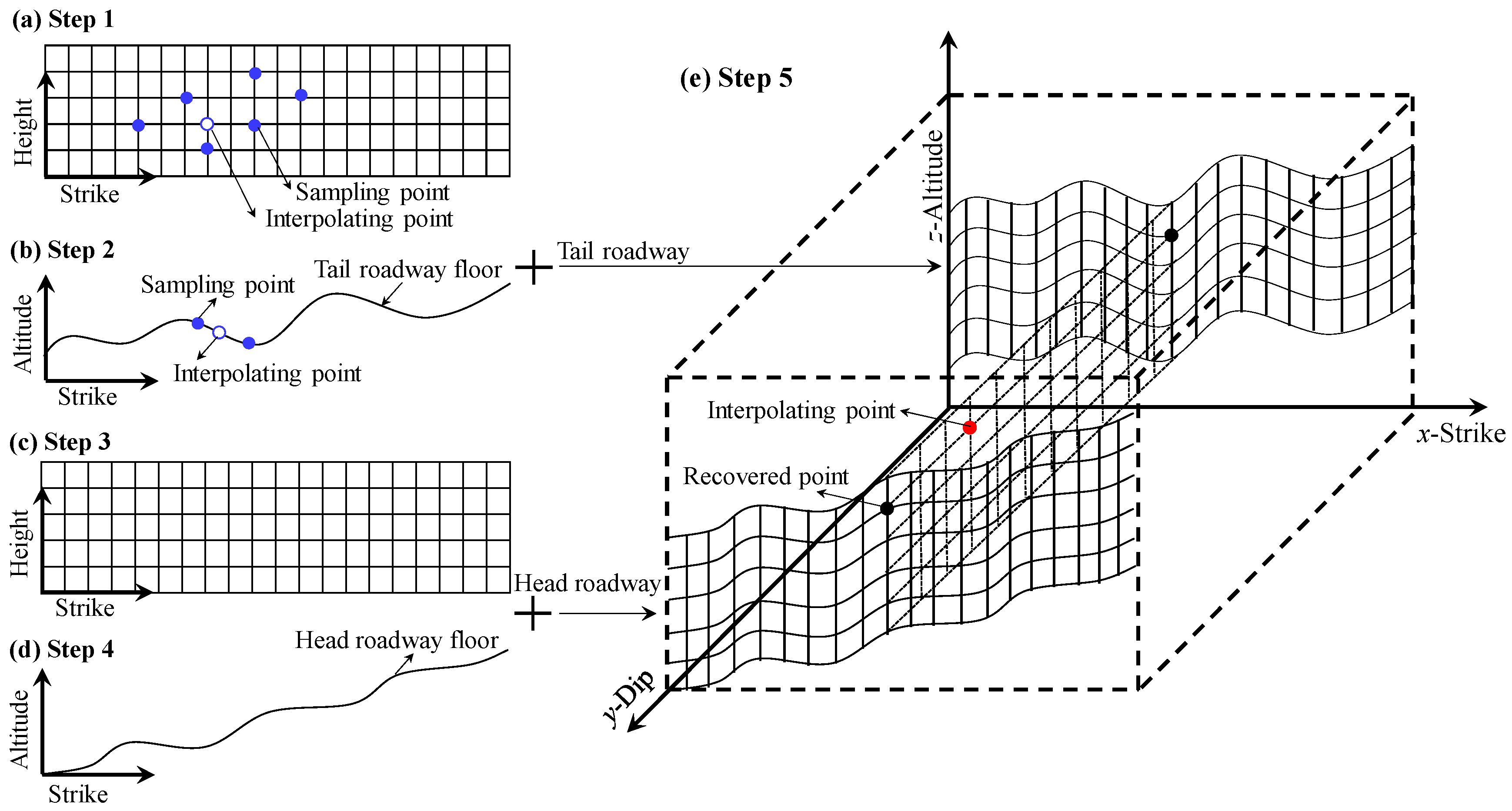
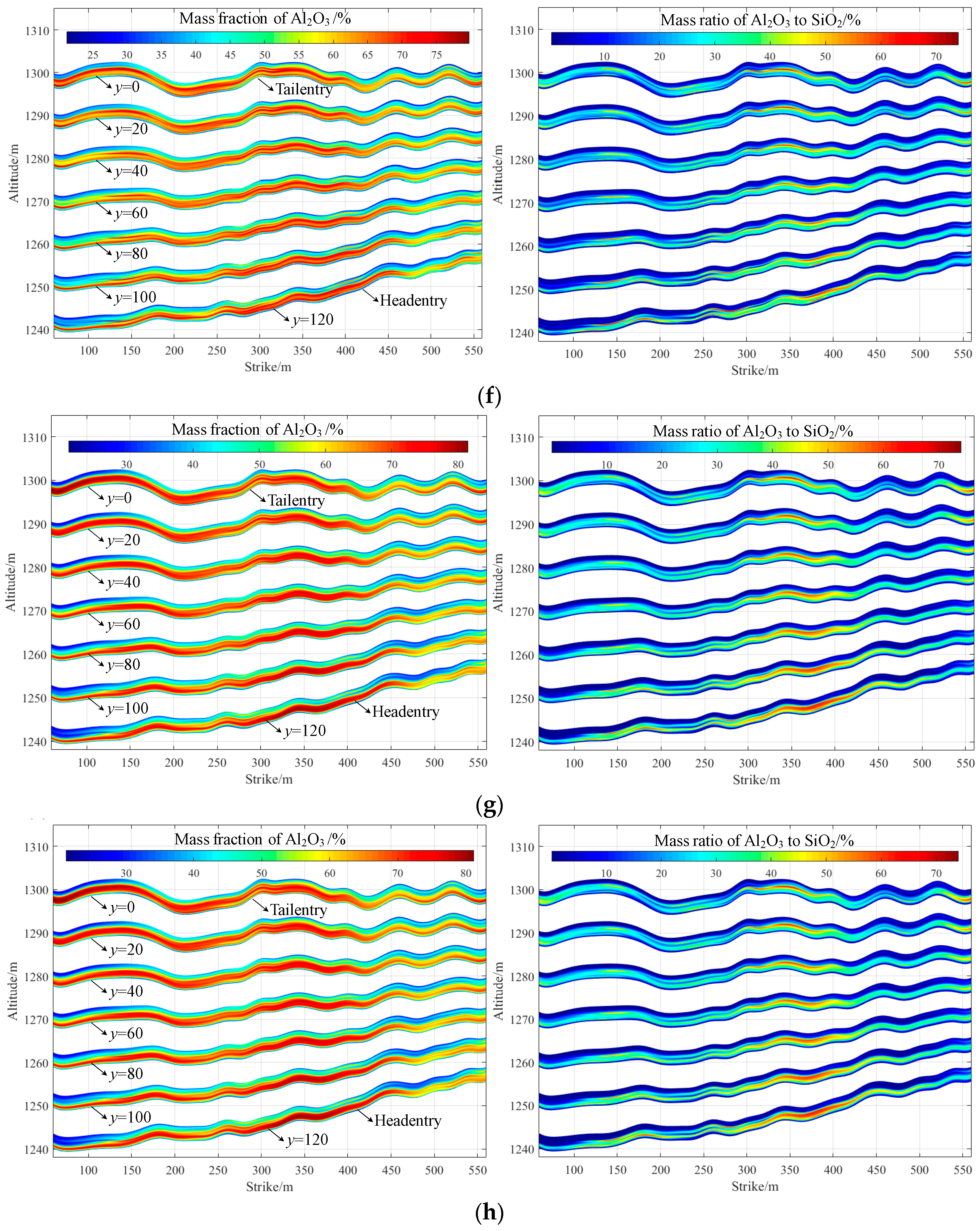
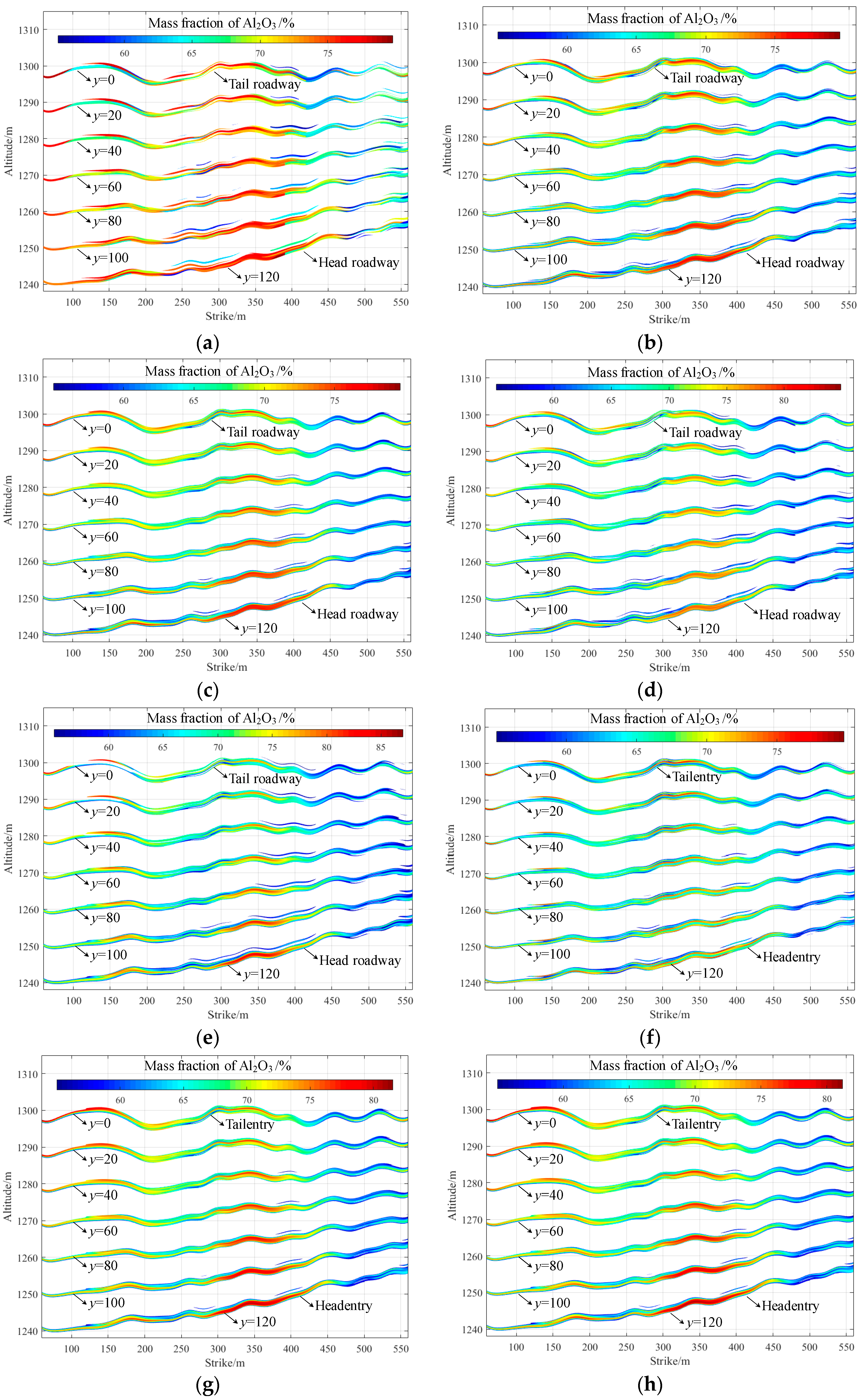
A multi-step interpolation algorithm was proposed to establish the grade distribution model of the mineralized seams in three dimensions. For a longwall mining panel with a U-shaped layout, where the tail and head roadways at both sides of the panel will be excavated beforehand, a five-step interpolation procedure was established. Firstly, the sample data with large variations and irregular distributions measured in the tail roadway were mapped into the nodes of a regular rectangular mesh grid and then used to estimate the over-sampled node data by conventional interpolation methods. Secondly, using a biharmonic spline method, the interpolated curve of the floor altitude of the tail roadway was established to recover interpolation data into the original frame. Thirdly, similar to the first step, the grade distribution data on the head roadway wall were interpolated. Fourthly, similar to the second step, the interpolation data were recovered by interpolated floor altitudes of the head roadway. Finally, the 3D distribution data between roadways were interpolated by a linear method.

(2)

During the first and the third steps, the nearest neighbor, linear, natural neighbor, cubic, biharmonic spline, IDW, SK, and OK interpolations were used to select which one is optimal for smooth and exact interpolations of the mineralized seams. A comparison of the differences between interpolated and sampled data—and between the field data from exploratory boreholes and corresponding interpolated data—showed that the stabilities of the interpolation curves decrease sequentially from natural neighbor, OK, SK, IDW, linear, cubic, and biharmonic spline, to the nearest neighbor methods. The multi-step interpolation using the natural neighbor method has an optimal stability and a minimal difference with the grade distribution in three dimensions. It seems that the natural neighbor interpolation has some predominant characteristics to be more physically realistic in the data interpolation.

(3)

Using the multi-step interpolation in which the natural neighbor method was selected to estimate the grade data distributed on the roadway wall, the ore reserve was estimated at 97,576 m³ with a mass fraction of Al₂O₃, marked as W_a, of 61.68% and a mass ratio of Al₂O₃ to SiO₂, marked as W_a/s, of 27.72. Subsequently, compared with the field data measured by the six exploratory boreholes, mean absolute errors, the root mean squared errors, and relative standard deviations of errors between interpolated and measured grade data are 2.544, 2.674, and 32.37% of W_a; and 1.761, 1.974, and 67.37% of W_a/s, respectively. On the whole, these differences are small relative to other methods.

References

1. Mortensen, M.E. Geometric Modeling; John Wiley & Sons Inc.: New York, NY, USA, 1985. [Google Scholar]
2. Calcagno, P.; Chilès, J.P.; Courrioux, G.; Guillen, A. Geological modelling from field data and geological knowledge Part I: Modelling method coupling 3D potential-field interpolation and geological rules. Phys. Earth Planet. Inter. 2008, 171, 147–157. [Google Scholar] [CrossRef]
3. Bascetin, A.; Tuylu, S.; Nieto, A. Influence of the ore block model estimation on the determination of the mining cutoff grade policy for sustainable mine production. Environ. Earth Sci. 2011, 64, 1409–1418. [Google Scholar] [CrossRef]
4. Franke, R. Scattered data interpolation: Tests of some methods. Math. Comput. 1982, 38, 181–200. [Google Scholar]
5. Myers, D.E. Spatial interpolation: An overview. Geoderma 1994, 62, 17–28. [Google Scholar] [CrossRef]
6. Goovaerts, P. Geostatistics for Natural Resources Evaluation; Oxford University Press: New York, NY, USA, 1997. [Google Scholar]
7. Sinclair, A.J.; Blackwell, G.H. Applied Mineral Inventory Estimation; Cambridge University Press: Cambridge, UK, 2002. [Google Scholar]
8. Abzalov, M. Applied Mining Geology; Springer International Publishing: Cham, Switzerland, 2016. [Google Scholar]
9. Deutsch, C.V. Geostatistical Reservoir Modeling; Oxford University Press: New York, NY, USA, 2002. [Google Scholar]
10. Zawadzki, J.; Fabijańczyk, P. Geostatistical evaluation of lead and zinc concentration in soils of an old mining area with complex land management. Int. J. Environ. Sci. Technol. 2013, 10, 729–742. [Google Scholar] [CrossRef]
11. Zawadzki, J.; Szuszkiewicz, M.; Fabijańczyk, P.; Magiera, T. Geostatistical discrimination between different sources of soil pollutants using a magneto-geochemical data set. Chemosphere 2016, 164, 668–676. [Google Scholar] [CrossRef] [PubMed]
12. Abramov, O.; Mcewen, A.S. An evaluation of interpolation methods for Mars Orbiter Laser Altimeter (MOLA) data. Int. J. Remote Sens. 2004, 25, 669–676. [Google Scholar] [CrossRef]
13. Sidik, N.A.C.; Attarzadeh, M.R.N. The use of cubic interpolation method for transient hydrodynamics of solid particles. Int. J. Eng. Sci. 2012, 51, 90–103. [Google Scholar]
14. Mahmoudabadi, H.; Izadi, M.; Menhaj, M.B. A hybrid method for grade estimation using genetic algorithm and neural networks. Comput. Geosci. 2009, 13, 91–101. [Google Scholar] [CrossRef]
15. Tutmez, B. An uncertainty oriented fuzzy methodology for grade estimation. Comput. Geosci. 2007, 33, 280–288. [Google Scholar] [CrossRef]
16. Gligorić, M.; Gligorić, Z.; Beljić, Č.; Torbica, S.; Štrbac Savić, S.; Nedeljković Ostojić, J. Multi-attribute technological modeling of coal deposits based on the fuzzy TOPSIS and C-mean clustering algorithms. Energies 2016, 9, 1059. [Google Scholar] [CrossRef]
17. Samanta, B.; Bandopadhyay, S. Construction of a radial basis function network using an evolutionary algorithm for grade estimation in a placer gold deposit. Comput. Geosci. 2009, 35, 1592–1602. [Google Scholar] [CrossRef]
18. Smirnoff, A.; Boisvert, E.; Paradis, S.J. Support vector machine for 3D modelling from sparse geological information of various origins. Comput. Geosci. 2008, 34, 127–143. [Google Scholar] [CrossRef]
19. Wang, Q.; Deng, J.; Liu, H.; Wang, Y.; Sun, X.; Wan, L. Fractal models for estimating local reserves with different mineralization qualities and spatial variations. J. Geochem. Explor. 2011, 108, 196–208. [Google Scholar] [CrossRef]
20. Sambridge, M.; Braun, J.; Mcqueen, H. Geophysical parametrization and interpolation of irregular data using natural neighbours. Geophys. J. Int. 1995, 122, 837–857. [Google Scholar] [CrossRef]
21. Peng, S.S. Longwall Mining, 2nd ed.; Society for Mining, Metallurgy, and Exploration, Inc. (SME): Englewood, CO, USA, 2006; pp. 1–20. [Google Scholar]
22. Karacan, C.Ö. Analysis of gob gas venthole production performances for strata gas control in longwall mining. Int. J. Rock Mech. Min. Sci. 2015, 79, 9–18. [Google Scholar] [CrossRef]
23. Islavath, S.R.; Deb, D.; Kumar, H. Numerical analysis of a longwall mining cycle and development of a composite longwall index. Int. J. Rock Mech. Min. Sci. 2016, 89, 43–54. [Google Scholar] [CrossRef]
24. Wang, S.; Li, X.; Wang, D. Mining-induced void distribution and application in the hydro-thermal investigation and control of an underground coal fire: A case study. Process Saf. Environ. Prot. 2016, 102, 734–756. [Google Scholar] [CrossRef]
25. Wang, S.; Li, X.; Wang, D. Void fraction distribution in overburden disturbed by longwall mining of coal. Environ. Earth Sci. 2016, 75, 151. [Google Scholar] [CrossRef]
26. Wang, S.; Li, X. Dynamic Distribution of Longwall Mining-Induced Voids in Overlying Strata of a Coalbed. Int. J. Geomech. 2016, 17. [Google Scholar] [CrossRef]
27. Wang, S.F.; Li, X.B.; Wang, S.Y.; Li, Q.Y.; Chen, C.; Feng, F.; Chen, Y. Three-dimensional orebody modelling and intellectualized longwall mining for stratiform bauxite deposits. Trans. Nonferr. Met. Soc. China 2016, 26, 2724–2730. [Google Scholar] [CrossRef]
28. Wang, S.; Li, X.; Du, K. Grade distribution and orebody demarcation of bauxite seam based on coupled Interpolation. Arab. J. Sci. Eng. 2017. [Google Scholar] [CrossRef]
29. Math Works. Matlab User Manual Version R2016b; Math Works: Natick, MA, USA, 2016. [Google Scholar]
30. Susanto, F.; de Souz, P.; He, J. Spatiotemporal interpolation for environmental modelling. Sensors 2016, 16, 1245. [Google Scholar] [CrossRef] [PubMed]
31. Burrough, P.A.; McDonnell, R.A. Principles of Geographical Information Systems; Oxford University Press: New York, NY, USA, 1998. [Google Scholar]
32. Sandwell, D.T. Biharmonic spline interpolation of GEOS-3 and SEASAT altimeter data. Geophys. Res. Lett. 1987, 14, 139–142. [Google Scholar] [CrossRef]
33. Administration of Quality Supervision, Inspection and Quarantine of the People’s Republic of China (AQSIQ). National Standard of the People’s Republic of China: Bauxite; Standard Press of China: Beijing, China, 2009.
Figure 1. Multi-step interpolation processes, including (a) a 2D interpolation for mineral grade on the tail roadway wall in the strike-height coordinate frame; (b) a 1D interpolation for interpolating floor altitudes of the tail roadway in the strike-altitude coordinate frame; (c) a 2D interpolation for the mineral grade on the head roadway wall in the strike-height coordinate frame; (d) a 1D interpolation for interpolating floor altitudes of the head roadway in the strike-altitude coordinate frame; and (e) a 3D linear interpolation for the mineral grade between roadways in the strike-dip-altitude coordinate frame.
Minerals 07 00071 g001
Figure 2. Layout of the 1102 longwall mining panel in the Wachangping bauxite mine.
Minerals 07 00071 g002
Figure 3. Position and grade data at scattered sampling points on the roadway walls.
Minerals 07 00071 g003
Figure 4. Slice maps of grade distributions at the cross-sections of y = 0, 20, 40, 60, 80, 100, and 120 m, based on the different 2D interpolation methods, including (a) nearest neighbor; (b) linear; (c) natural neighbor; (d) cubic; (e) biharmonic spline; (f) IDW; (g) SK; and (h) OK interpolations.
Minerals 07 00071 g004aMinerals 07 00071 g004bMinerals 07 00071 g004c
Figure 5. Slice maps of delimited orebody at the cross-sections of y = 0, 20, 40, 60, 80, 100, and 120 m, based on the different 2D interpolation methods, including (a) nearest neighbor; (b) linear; (c) natural neighbor; (d) cubic; (e) biharmonic spline; (f) IDW; (g) SK; and (h) OK interpolations.
Minerals 07 00071 g005