Mineralogical Characterization and Dissolution Experiments in Gamble’s Solution of Tremolitic Amphibole from Passo di Caldenno (Sondrio, Italy)

 , , , ,
Abstract
:1. Introduction
Geological Setting
2. Materials and Methods
2.1. VLM
2.2. XRPD
2.3. EPMA
2.4. µ-Raman and FTIR Spectroscopy
2.5. BET Surface Area Analysis
2.6. Laser Diffraction
2.7. FE-ESEM-EDXS
2.8. ICP-OES
3. Results
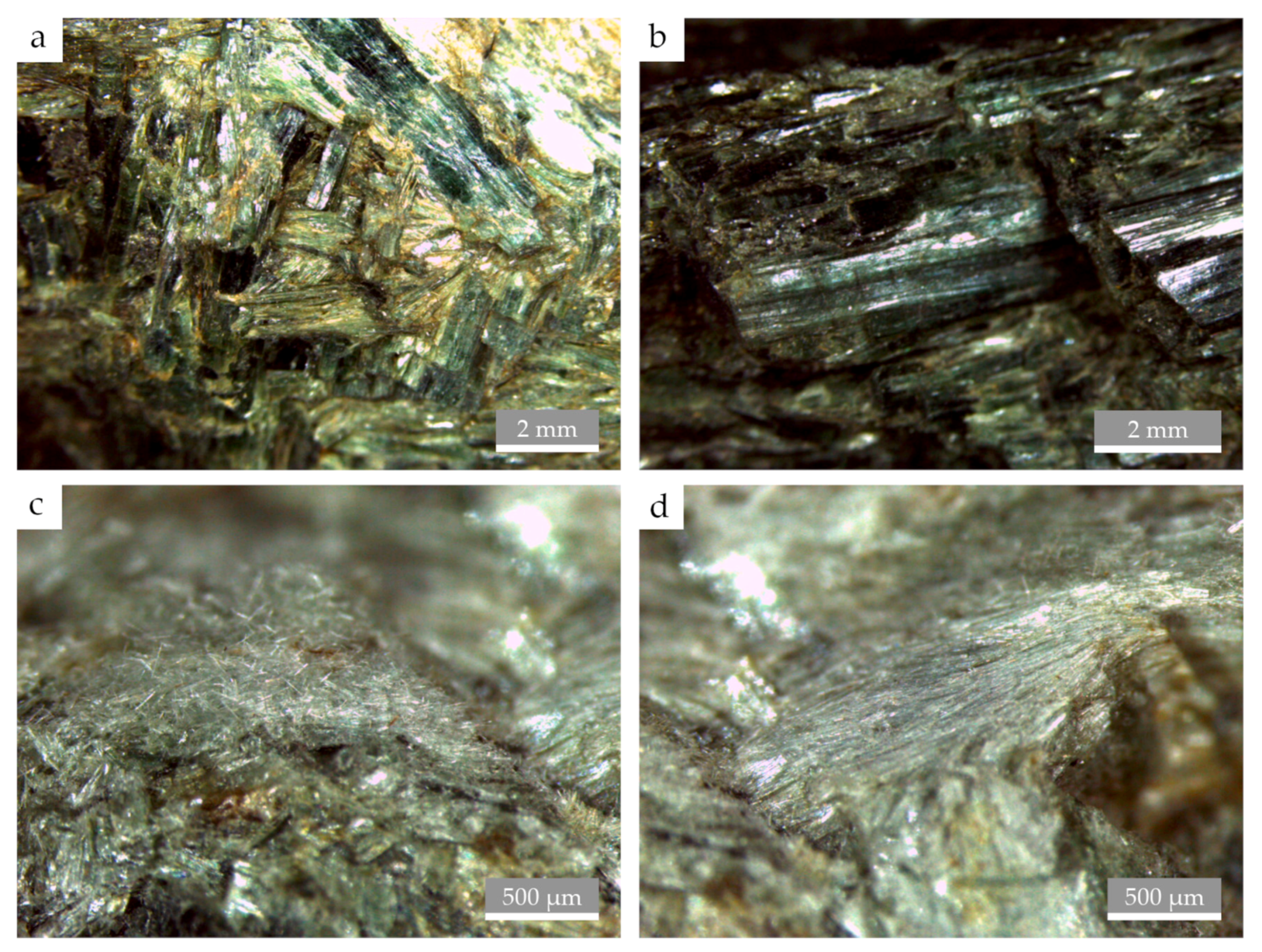
3.1. Naked-Eye and VLM Description of the Sample
3.2. XRPD
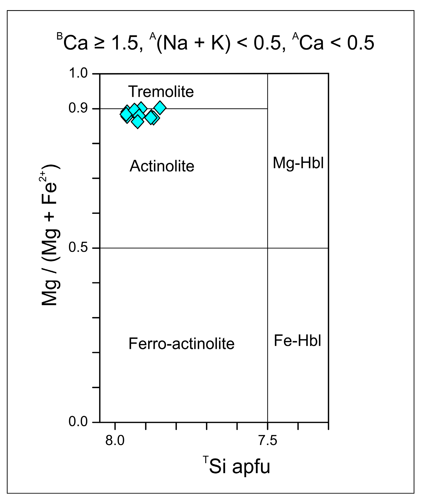
3.3. EPMA
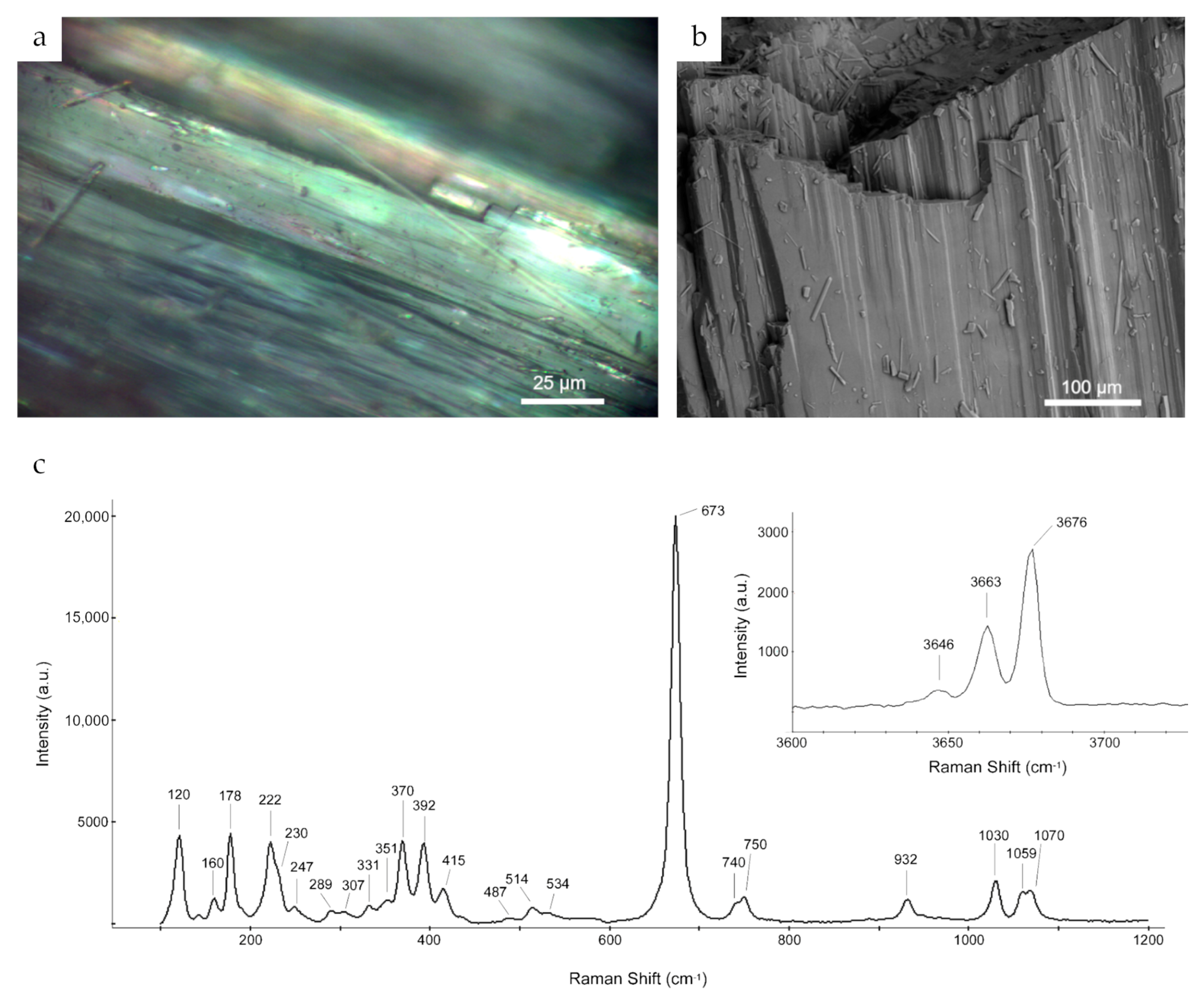
3.4. µ-Raman and FTIR Spectroscopic Observations
3.5. BET Surface Area Results
3.6. Particle-Size Distribution
3.7. Morphology as Observed by FE-ESEM for the Powdered Starting Material
3.8. Dimensional Results Obtained by FE-ESEM for the Powdered Starting Material
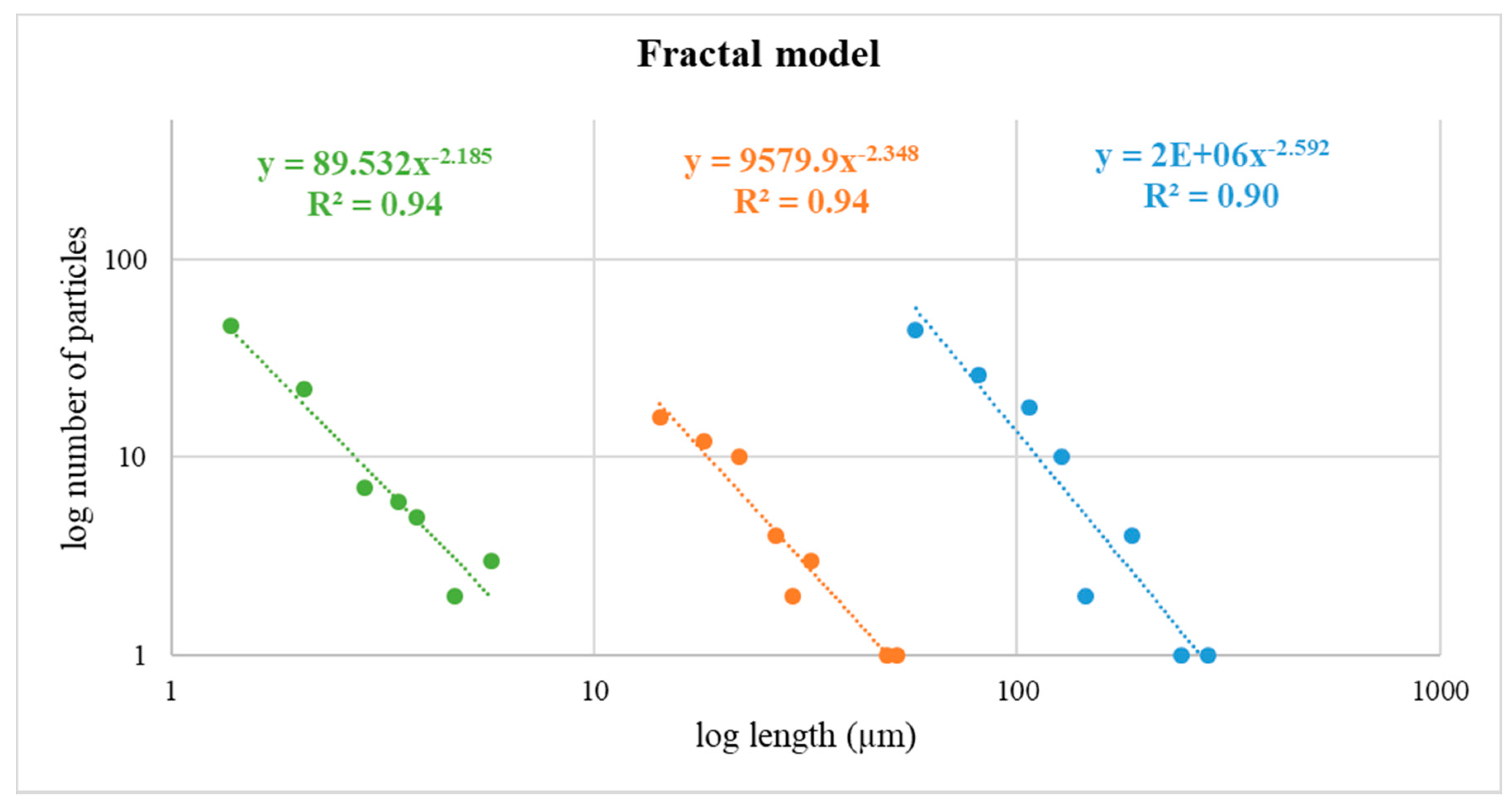
3.9. Fractal Model from FE-ESEM Data Obtained for the Powdered Starting Material
3.10. ICP-OES Data from Dissolution Experiment
3.11. Morphology as Observed by FE-ESEM for the Material After Dissolution Experiment
3.12. Dimensional Results Obtained by FE-ESEM for the Material after Dissolution Experiment
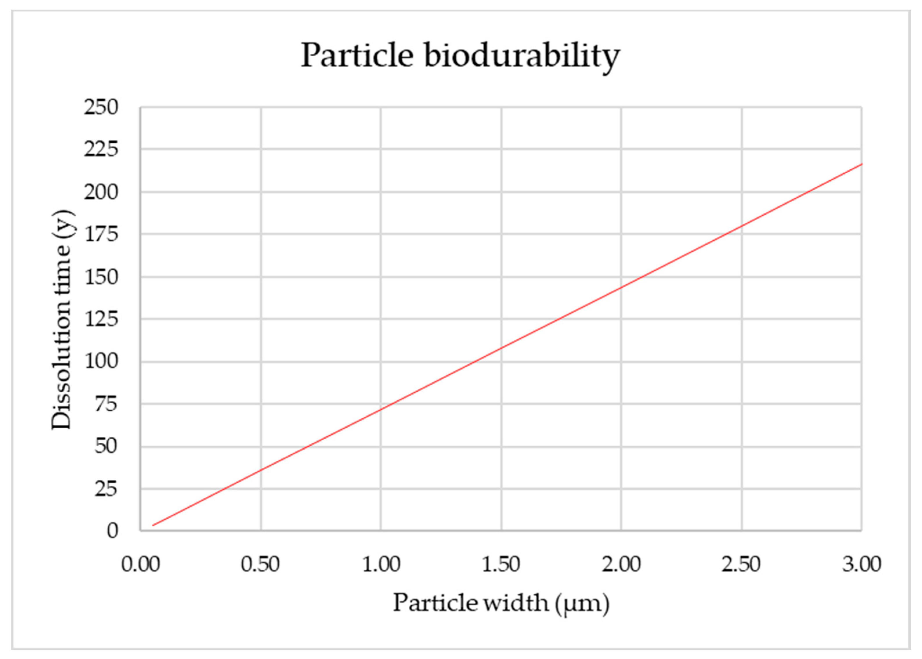
3.13. Estimation of Fiber Biodurability
4. Discussion
5. Conclusions
Supplementary Materials
Author Contributions
Funding
Acknowledgments
Conflicts of Interest
References
- Gamble, J.F.; Gibbs, G.W.; Nolan, R.P. An evaluation of the risk of lung cancer and mesothelioma from exposure to amphibole cleavage fragments. Regul. Toxicol. Pharmacol. 2008, 52, S154–S186. [Google Scholar] [CrossRef] [PubMed]
- Gualtieri, A.F. (Ed.) Introduction. In Mineral Fibres: Crystal Chemistry, Chemical-Physical Properties, Biological Interaction and Toxicity (EMU Notes in Mineralogy); European Mineralogical Union: London, UK, 2017; Volume 18, pp. 1–15. ISBN 9780903056656. [Google Scholar]
- Ferro, A.; Zebedeo, C.N.; Davis, C.; Ng, K.W.; Pfau, J.C. Amphibole, but not chrysotile, asbestos induces anti-nuclear autoantibodies and IL-17 in C57BL/6 mice. J. Immunotoxicol. 2014, 11, 283–290. [Google Scholar] [CrossRef] [PubMed]
- Pfau, J.C.; Serve, K.M.; Noonan, C.W. Autoimmunity and asbestos exposure. Autoimmune Dis. 2014, 2014, 782045. [Google Scholar] [CrossRef] [PubMed]
- Meeker, G.P.; Bern, A.M.; Brownfield, I.K.; Lowers, H.A.; Sutley, S.J.; Hoefen, T.M.; Vance, J.S. The composition and morphology of amphiboles from the Rainy Creek complex, near Libby, Montana. Am. Mineral. 2003, 88, 1955–1969. [Google Scholar] [CrossRef]
- Boulanger, M.; Morlais, F.; Bouvier, V.; Galateau-Salle, F.; Guittet, L.; Maquignon, M.; Paris, C.; Raffaelli, C.; Launoy, G.; Clin, B. O32-1 Digestive cancers and occupational asbestos exposure: Significant associations in a French cohort of asbestos plant workers. Occup. Environ. Med. 2016, 73, A58. [Google Scholar] [CrossRef]
- Clin, B.; Thaon, I.; Boulanger, M.; Brochard, P.; Chamming’s, S.; Gislard, A.; Lacourt, A.; Luc, A.; Ogier, G.; Paris, C.; Pairon, J. Cancer of the esophagus and asbestos exposure. Am. J. Ind. Med. 2017, 60, 968–975. [Google Scholar] [CrossRef] [PubMed]
- Di Ciaula, A. Asbestos ingestion and gastrointestinal cancer: A possible underestimated hazard. Expert Rev. Gastroenterol. Hepatol. 2017, 11, 419–425. [Google Scholar] [CrossRef] [PubMed]
- Paris, C.; Thaon, I.; Hérin, F.; Clin, B.; Lacourt, A.; Luc, A.; Coureau, G.; Brochard, P.; Chamming’s, S.; Gislard, A.; et al. Occupational asbestos exposure and incidence of colon and rectal cancers in French men: The asbestos-related diseases cohort (ARDCo-Nut). Environ. Health Perspect. 2017, 3, 409–415. [Google Scholar] [CrossRef] [PubMed]
- Gunter, M.E.; Belluso, E.; Mottana, A. Amphiboles: Environmental and health concerns. Rev. Mineral. Geochem. 2007, 67, 453–516. [Google Scholar] [CrossRef]
- Martin, R.F. Amphiboles in the igneous environment. Rev. Mineral. Geochem. 2007, 67, 323–358. [Google Scholar] [CrossRef]
- Schumacher, J.C. Metamorphic amphiboles: Composition and coexistence. Rev. Mineral. Geochem. 2007, 67, 359–416. [Google Scholar] [CrossRef]
- Vignaroli, G.; Rossetti, F.; Belardi, G.; Billi, A. Linking rock fabric to fibrous mineralisation: A basic tool for the asbestos hazard. Nat. Hazard Earth Syst. 2011, 11, 1267–1280. [Google Scholar] [CrossRef] [Green Version]
- Vignaroli, G.; Ballirano, P.; Belardi, G.; Rossetti, F. Asbestos fibre identification vs. evaluation of asbestos hazard in ophiolitic rock mélanges; a case study from the Ligurian Alps (Italy). Environ. Earth Sci. 2014, 72, 3679–3698. [Google Scholar] [CrossRef]
- Trommsdorff, V.; Montrasio, A.; Hermann, J.; Müntener, O.; Spillman, P.; Gieré, R. The geological map of Valmalenco. Schweiz. Mineral. Petrogr. Mitt. 2005, 85, 1–13. [Google Scholar]
- Trommsdorff, V.; Evans, B.W. Antigorite-ophicarbonates: Contact metamorphism in Valmalenco, Italy. Contrib. Mineral. Petrol. 1977, 62, 301–312. [Google Scholar] [CrossRef]
- Hermann, J.; Müntener, O.; Trommsdorff, V.; Hansmann, W.; Piccardo, G.B. Fossil crust-to-mantle transition, Val Malenco (Italian Alps). J. Geophys. Res-Solid Earth 1997, 102, 20123–20132. [Google Scholar] [CrossRef] [Green Version]
- Bocchio, R.; Diella, V.; Adamo, I.; Marinoni, N. Mineralogical characterization of the gem-variety pink clinozoisite from Val Malenco, Central Alps, Italy. Rend. Fis. Acc. Lincei 2017, 28, 549–557. [Google Scholar] [CrossRef]
- Trommsdorff, V.; Evans, B.W. Titanian hydroxyl-clinohumite: Formation and breakdown in antigorite rocks (Malenco, Italy). Contrib. Mineral. Petrol. 1980, 72, 229–242. [Google Scholar] [CrossRef]
- Wojydr, M. Fityk: A general purpose peak fitting program. J. Appl. Crystallogr. 2010, 42, 1126–1128. [Google Scholar] [CrossRef]
- Marques, M.R.C.; Loebenberg, R.; Almukainzi, M. Simulated biological fluids with possible application in dissolution testing. Dissolut. Technol. 2011, 18, 15–28. [Google Scholar] [CrossRef]
- Pacella, A.; Fantauzzi, M.; Turci, F.; Cremisini, C.; Montereali, M.R.; Nardi, E.; Atzei, D.; Rossi, A.; Andreozzi, G.B. Dissolution reaction and surface iron speciation of UICC crocidolite in buffered solution at pH 7.4: A combined ICP-OES, XPS and TEM investigation. Geochim. Cosmochim. Acta 2014, 127, 221–232. [Google Scholar] [CrossRef]
- Della Ventura, G.; Vigliaturo, R.; Gieré, R.; Pollastri, S.; Gualtieri, A.F.; Iezzi, G. Infrared spectroscopy of the regulated asbestos amphiboles. Minerals 2018, 8, 413. [Google Scholar] [CrossRef]
- Oberti, R.; Cannillo, E.; Toscani, G. How to name amphiboles after the IMA 2012 report: Rules of thumb and a new PC program for monoclinic amphiboles. Periodico Mineral. 2012, 81, 257–267. [Google Scholar] [CrossRef]
- Locock, A.J. An Excel spreadsheet to classify chemical analyses of amphiboles following the IMA 2012 recommendations. Comput. Geosci. 2014, 62, 1–11. [Google Scholar] [CrossRef]
- Hawthorne, F.C.; Oberti, R.; Harlow, G.E.; Maresch, W.V.; Martin, R.F.; Schumacher, J.C.; Welch, M. IMA Report: Nomenclature of the amphibole supergroup. Am. Mineral. 2012, 9, 2031–2048. [Google Scholar] [CrossRef]
- Leake, B.E.; Woolley, A.R.; Arps, C.E.; Birch, W.D.; Gilbert, M.C.; Grice, J.D.; Hawthorne, F.C.; Kisch, H.J.; Krivovichev, V.G. Nomenclature of amphiboles: Report of the subcommittee on amphiboles of the International Mineralogical Association commission on new minerals and mineral names. Mineral. Mag. 1997, 61, 295–321. [Google Scholar] [CrossRef]
- Leake, B.E.; Woolley, A.R.; Birch, W.D.; Burke, E.A.; Ferraris, G.; Grice, J.D.; Hawthorne, F.C.; Kisch, H.J.; Krivovichev, V.G.; Schumacher, J.C.; et al. Nomenclature of amphiboles: Additions and revisions to the International Mineralogical Associations amphibole nomenclature. Mineral. Mag. 2004, 68, 209–215. [Google Scholar] [CrossRef]
- Lucci, F.; Della Ventura, G.; Conte, A.; Nazzari, M.; Scarlato, P. Naturally Occurring Asbestos (NOA) in Granitoid Rocks, A Case Study from Sardinia (Italy). Minerals 2018, 8, 442. [Google Scholar] [CrossRef]
- Rinaudo, C.; Belluso, E.; Gastaldi, D. Assessment of the use of Raman spectroscopy for the determination of amphibole asbestos. Mineral. Mag. 2004, 68, 455–465. [Google Scholar] [CrossRef]
- Apopei, A.I.; Buzgar, N.; Buzatu, A. Raman and infrared spectroscopy of kaersutite and certain common amphiboles. Analele Stiintifice ale Universitatii “Al. I. Cuza” din Iasi. Seria Geologie 2011, 57, 35–58. [Google Scholar]
- Della Ventura, G. The analysis of asbestos minerals using vibrational spectroscopies (FTIR, Raman): Crystal Chemistry, identification and environmental applications. In Mineral Fibres: Crystal Chemistry, Chemical-Physical Properties, Biological Interaction and Toxicity (EMU Notes in Mineralogy); Gualtieri, A.F., Ed.; European Mineralogical Union: London, UK, 2017; Volume 18, pp. 135–169. ISBN 9780903056656. [Google Scholar]
- Ishida, K.; Jenkins, D.M.; Hawthorne, F.C. Mid-IR bands of synthetic calcic amphiboles of tremolite-pargasite series and of natural calcic amphiboles. Am. Mineral. 2008, 93, 1112–1118. [Google Scholar] [CrossRef]
- Kouropis-Agalou, K.; Liscio, A.; Treossi, E.; Ortolani, L.; Pugno, N.M.; Palermo, V. Fragmentation and exfoliation of 2-dimensional materials: A statistical approach. Nanoscale 2014, 6, 5926–5933. [Google Scholar] [CrossRef] [PubMed]
- Gonda, I.; Abd El Khalik, A.F. On the calculation of aerodynamic diameters of fibers. Aerosol Sci. Technol. 1985, 4, 233–238. [Google Scholar] [CrossRef]
- Veblen, D.R.; Wylie, A.G. Mineralogy of amphiboles and 1:1 layer silicates. In Reviews in Mineralogy and Geochemistry; Guthrie, G.D., Jr., Mossman, B.T., Eds.; Mineralogical Society of America: Chantilly, VA, USA, 1993; Volume 28, pp. 61–137. ISSN 0275-0279. [Google Scholar]
- National Institute for Occupational Safety and Health (NIOSH). Asbestos Fibers and Other Elongated Mineral Particles: State of the Science and Roadmap for Research; DHHS Publication No.2011-159; 2011. Available online: https://www.cdc.gov/niosh/docs/2011-159/pdfs/2011-159.pdf (accessed on 28 November 2018).
- Wylie, A.G. Modeling asbestos population: A fractal approach. Canad. Mineral. 1993, 30, 437–446. [Google Scholar]
- Rozalen, M.; Ramos, M.E.; Gervilla, F.; Kerestedjian, T.; Fiore, S.; Huertas, F.J. Dissolution study of tremolite and anthophyllite: pH effect on the reaction kinetics. Appl. Geochem. 2014, 49, 46–56. [Google Scholar] [CrossRef]
- Bernstein, D.M.; Castranova, V.; Donaldson, K.; Fubini, B.; Hadley, J.; Hesterberg, T.; Kaneg, A.; Laih, D.; McConnell, E.E.; Muhle, H.; et al. Testing of fibrous particles: Short-term assays and strategies. Inhal. Toxicol. 2005, 17, 497–537. [Google Scholar] [CrossRef] [PubMed]
- Hume, L.A.; Rimstidt, J.D. The biodurability of chrysotile asbestos. Am. Mineral. 1992, 77, 1125–1128. [Google Scholar]
- Rozalen, M.; Ramos, M.E.; Huertas, F.J.; Fiore, S.; Gervilla, F. Dissolution kinetics and biodurability of tremolite particles in mimicked lung fluids: Effect of citrate and oxalate. J. Asian Earth Sci. 2013, 77, 318–326. [Google Scholar] [CrossRef]
- Critelli, T.; Marini, L.; Schott, J.; Mavromatis, V.; Apollaro, C.; Rinder, T.; De Rosa, R.; Oelkers, E.H. Dissolution rates of actinolite and chlorite from a whole-rock experimental study of metabasalt dissolution from 2 ≤ pH ≤ 12 at 25 °C. Chem. Geol. 2014, 390, 100–108. [Google Scholar] [CrossRef]
- Pollastri, S.; Gualtieri, A.F.; Lasinantti Gualtieri, M.; Hanuskova, M.; Cavallo, A.; Gaudino, G. The zeta potential of mineral fibres. J. Hazard. Mater. 2014, 276, 469–479. [Google Scholar] [CrossRef] [PubMed]
- Pacella, A.; Fantauzzi, M.; Turci, F.; Cremisini, C.; Montereali, M.R.; Nardi, E.; Atzei, D.; Rossi, A.; Andreozzi, G.B. Surface alteration mechanism and topochemistry of iron in tremolite asbestos: A step toward understanding the potential hazard of amphibole asbestos. Chem. Geol. 2015, 405, 28–38. [Google Scholar] [CrossRef]


| Oxides | Average (n = 12 with σn−1 in Parentheses) | Range |
|---|---|---|
| SiO2 (wt. %) | 56.68 (0.67) | 55.65–57.72 |
| TiO2 | <0.01 | - |
| Al2O3 | 0.46 (0.07) | 0.29–0.54 |
| FeOt | 5.37 (0.75) | 4.44–6.59 |
| MnO | 0.19 (0.04) | 0.13–0.26 |
| MgO | 21.16 (0.35) | 20.58–21.62 |
| CaO | 13.12 (0.29) | 12.58–13.74 |
| Na2O | 0.25 (0.08) | 0.03–0.36 |
| K2O | 0.03 (0.02) | 0.00–0.06 |
| F | 0.06 (0.01) | 0.00–0.22 |
| Cl | <0.01 | - |
| Total | 97.32 | 96.47–98.16 |
| Normalization Scheme: 13-CNK, all ferrous iron | ||
| Si, apfu | 7.92 | 7.85–7.96 |
| Al | 0.07 | 0.04–0.09 |
| ΣT | 7.99 | 7.94–8.00 |
| Al | 0.01 | 0.00–0.04 |
| Mn2+ | 0.01 | 0.00–0.02 |
| Fe2+ | 0.58 | 0.49–0.69 |
| Mg | 4.41 | 4.31–4.51 |
| ΣC | 5.00 | 5.00 |
| Mn2+ | 0.02 | 0.00–0.03 |
| Fe2+ | 0.05 | 0.00–0.12 |
| Ca | 1.96 | 1.89–1.99 |
| ΣB | 2.03 | 2.00–2.13 |
| Na | 0.07 | 0.01–0.09 |
| K | 0.01 | 0.00–0.01 |
| ΣA | 0.08 | 0.01–0.10 |
| OH | 1.98 | 1.90–2.00 |
| F | 0.02 | 0.00–0.10 |
| ΣW | 2.00 | 2.00 |
| Mg/(Mg+Fe2+) | 0.88 | 0.86–0.90 |
| Laser Diffraction Dimensional Distribution | Geometric | Logarithmic |
| µm | ɸ | |
| Mode 1: | 127.79 | 2.97 |
| Mode 2: | 73.02 | 3.78 |
| Mode 3: | - | - |
| D10: | 4.53 | 2.57 |
| Median or D50: | 49.78 | 4.33 |
| D90: | 168.75 | 7.79 |
| (D90/D10): | 37.25 | 3.03 |
| (D90-D10): | 164.22 | 5.22 |
| (D75/D25): | 6.45 | 1.83 |
| (D75-D25): | 90.44 | 2.69 |
| Folk & Ward Method | ||
| Geometric | Logarithmic | |
| µm | ɸ | |
| Mean | 39.21 | 4.67 |
| Sorting (σ) | 4.13 | 2.05 |
| Skewness (Sk) | −0.34 | 0.34 |
| Kurtosis (K) | 1.05 | 1.05 |
| Magnification 102× (n = 150) | ||||||||
| ESEM Dimensional Study | L | w | L/w | Areal | Acalc | Areal/Acalc | s (Areal) | Dae |
| Mean | 75.03 | 26.00 | 4.53 | 2141.08 | 2396.60 | 0.88 | 38.69 | 54.68 |
| Median | 61.56 | 17.75 | 3.18 | 1061.42 | 1181.89 | 0.91 | 32.58 | 44.09 |
| Mode | #N/D | 43.50 | #N/D | #N/D | #N/D | #N/D | #N/D | #N/D |
| Max | 336.27 | 162.91 | 33.37 | 31031.81 | 31038.24 | 1.00 | 176.16 | 256.19 |
| Min | 16.00 | 1.18 | 0.73 | 21.19 | 25.48 | 0.58 | 4.60 | 3.93 |
| Std. Dev. | 47.60 | 24.98 | 4.26 | 3660.95 | 3976.48 | 0.10 | 25.47 | 39.57 |
| Std. Error | 3.89 | 2.04 | 0.35 | 298.92 | 324.68 | 0.01 | 2.08 | 3.23 |
| Magnification 103× (n = 150) | ||||||||
| L | w | L/w | Areal | Acalc | Areal/Acalc | s (Areal) | Dae | |
| Mean | 11.80 | 3.92 | 5.24 | 57.15 | 66.36 | 0.86 | 5.86 | 8.34 |
| Median | 8.52 | 2.80 | 3.47 | 18.50 | 22.35 | 0.90 | 4.30 | 6.13 |
| Mode | 8.18 | 0.75 | #N/D | #N/D | #N/D | #N/D | #N/D | #N/D |
| Max | 54.63 | 23.67 | 33.75 | 1046.30 | 1082.56 | 1.00 | 32.35 | 46.28 |
| Min | 2.00 | 0.20 | 0.33 | 0.58 | 0.63 | 0.11 | 0.76 | 0.71 |
| Std. Dev. | 9.13 | 3.99 | 5.43 | 114.36 | 125.81 | 0.14 | 4.79 | 7.21 |
| Std. Error | 0.75 | 0.33 | 0.44 | 9.34 | 10.27 | 0.01 | 0.39 | 0.59 |
| Magnification 104× (n = 150) | ||||||||
| L | w | L/w | Areal | Acalc | Areal/Acalc | s (Areal) | Dae | |
| Mean | 1.87 | 0.59 | 4.03 | 1.07 | 1.40 | 0.87 | 0.87 | 1.26 |
| Median | 1.29 | 0.47 | 2.52 | 0.53 | 0.60 | 0.89 | 0.72 | 1.03 |
| Mode | 0.92 | 0.41 | #N/D | 0.20 | #N/D | #N/D | 0.45 | #N/D |
| Max | 41.56 | 2.35 | 59.73 | 10.38 | 28.92 | 1.00 | 3.22 | 5.18 |
| Min | 0.15 | 0.05 | 0.85 | 0.01 | 0.01 | 0.09 | 0.11 | 0.17 |
| Std. Dev. | 3.44 | 0.44 | 5.50 | 1.62 | 2.93 | 0.12 | 0.56 | 0.89 |
| Std. Error | 0.28 | 0.04 | 0.45 | 0.13 | 0.24 | 0.01 | 0.05 | 0.07 |
| Magnification | Acicular % | Bladed % | Columnar % | Equant % | Fiber % | Massive % | Platy % | Prismatic % |
|---|---|---|---|---|---|---|---|---|
| 102× | 7.33 | 16.00 | 12.67 | 10.67 | 21.33 | 6.67 | 4.00 | 21.33 |
| 103× | 14.00 | 20.67 | 6.67 | 10.00 | 15.33 | 6.00 | 12.00 | 15.33 |
| 104× | 11.33 | 29.33 | 13.33 | 9.33 | 6.67 | 9.33 | 4.00 | 16.67 |
| Atomic % Ratios | Powdered Starting Material (Bulk EPMA) | Powdered Starting Material (Bulk EDXS) | Powdered Sample after 168-h Exposure (Bulk EDXS) | Gamble’s Solution after 168-h Experiment (ICP-OES) |
|---|---|---|---|---|
| 0.56 (0.01) | 0.63 (0.1) | 0.64 (0.1) | 0.51 (0.04) | |
| 0.25 (0.01) | 0.29 (0.07) | 0.41 (0.2) | 0.11 (0.03) | |
| 0.08 (0.01) | 0.12 (0.09) | 0.22 (0.2) | 0.030 (0.01) |
| Magnification 102× (n = 150) | ||||||||
| ESEM Dimensional Study | L | w | L/w | Areal | Acalc | Areal/Acalc | s (Areal) | Dae |
| Mean | 115.18 | 31.09 | 5.34 | 3652.20 | 4201.40 | 0.85 | 52.48 | 72.56 |
| Median | 107.94 | 28.31 | 4.02 | 2762.68 | 3081.09 | 0.90 | 52.56 | 68.32 |
| Mode | #N/D | 6.25 | #N/D | 93.99 | #N/D | #N/D | 9.69 | #N/D |
| Max | 462.15 | 94.95 | 40.56 | 22437.60 | 30946.22 | 1.00 | 149.79 | 198.56 |
| Min | 13.52 | 1.40 | 1.06 | 15.63 | 19.87 | 0.12 | 3.95 | 4.28 |
| Std. Dev. | 71.68 | 21.77 | 5.15 | 3776.07 | 4436.00 | 0.16 | 30.07 | 43.61 |
| Std. Error | 5.85 | 1.78 | 0.42 | 308.31 | 362.20 | 0.01 | 2.46 | 3.56 |
| Magnification 103× (n = 150) | ||||||||
| L | w | L/w | Areal | Acalc | Areal/Acalc | s (Areal) | Dae | |
| Mean | 17.70 | 6.12 | 3.72 | 144.19 | 171.05 | 0.85 | 8.95 | 13.22 |
| Median | 10.66 | 4.37 | 2.63 | 33.27 | 41.13 | 0.88 | 5.77 | 8.90 |
| Mode | 4.44 | 1.90 | #N/D | 71.60 | #N/D | #N/D | 8.46 | #N/D |
| Max | 154.49 | 41.94 | 34.43 | 2188.56 | 2369.54 | 1.00 | 46.78 | 69.59 |
| Min | 1.57 | 0.19 | 1.04 | 0.58 | 0.60 | 0.08 | 0.76 | 0.62 |
| Std. Dev. | 19.39 | 6.11 | 3.76 | 298.25 | 343.70 | 0.13 | 8.03 | 11.98 |
| Std. Error | 1.58 | 0.50 | 0.31 | 24.35 | 28.06 | 0.01 | 0.66 | 0.98 |
| Magnification 104× (n = 150) | ||||||||
| L | w | L/w | Areal | Acalc | Areal/Acalc | s (Areal) | Dae | |
| Mean | 3.64 | 1.38 | 3.12 | 6.19 | 7.66 | 0.83 | 1.95 | 3.00 |
| Median | 2.73 | 1.15 | 2.27 | 2.71 | 3.17 | 0.86 | 1.65 | 2.45 |
| Mode | 2.30 | 0.15 | #N/D | #N/D | #N/D | #N/D | #N/D | #N/D |
| Max | 19.99 | 6.85 | 15.25 | 74.16 | 102.53 | 1.00 | 8.61 | 14.88 |
| Min | 0.14 | 0.02 | 1.11 | 0.00 | 0.01 | 0.11 | 0.03 | 0.06 |
| Std. Dev. | 3.34 | 1.14 | 2.39 | 10.55 | 13.38 | 0.15 | 1.55 | 2.41 |
| Std. Error | 0.27 | 0.09 | 0.20 | 0.86 | 1.09 | 0.01 | 0.13 | 0.20 |
| Magnification | Acicular % | Bladed % | Columnar % | Equant % | Fiber % | Massive % | Platy % | Prismatic % |
|---|---|---|---|---|---|---|---|---|
| 102× | 10.67 | 19.33 | 13.33 | 9.33 | 22.67 | 8.67 | 0.67 | 15.33 |
| 103× | 10.67 | 24.67 | 10.67 | 12.00 | 14.67 | 8.00 | 4.00 | 15.33 |
| 104× | 10.67 | 26.00 | 19.33 | 11.33 | 6.00 | 10.67 | 0.67 | 15.33 |
© 2018 by the authors. Licensee MDPI, Basel, Switzerland. This article is an open access article distributed under the terms and conditions of the Creative Commons Attribution (CC BY) license (http://creativecommons.org/licenses/by/4.0/).
Share and Cite
Vigliaturo, R.; Della Ventura, G.; Choi, J.K.; Marengo, A.; Lucci, F.; O'Shea, M.J.; Pérez-Rodríguez, I.; Gieré, R. Mineralogical Characterization and Dissolution Experiments in Gamble’s Solution of Tremolitic Amphibole from Passo di Caldenno (Sondrio, Italy). Minerals 2018, 8, 557. https://doi.org/10.3390/min8120557
Vigliaturo R, Della Ventura G, Choi JK, Marengo A, Lucci F, O'Shea MJ, Pérez-Rodríguez I, Gieré R. Mineralogical Characterization and Dissolution Experiments in Gamble’s Solution of Tremolitic Amphibole from Passo di Caldenno (Sondrio, Italy). Minerals. 2018; 8(12):557. https://doi.org/10.3390/min8120557
Chicago/Turabian StyleVigliaturo, Ruggero, Giancarlo Della Ventura, Jessica K. Choi, Alessandra Marengo, Federico Lucci, Michael J. O'Shea, Ileana Pérez-Rodríguez, and Reto Gieré. 2018. "Mineralogical Characterization and Dissolution Experiments in Gamble’s Solution of Tremolitic Amphibole from Passo di Caldenno (Sondrio, Italy)" Minerals 8, no. 12: 557. https://doi.org/10.3390/min8120557