1. Introduction
Multiple-point statistics (MPS) allows the simulation of spatial or temporal random functions by reproducing pattern statistics from an exhaustive data set — the training image (TI) — built from conceptual knowledge [
1] or borrowed from analogue sites [
2,
3]. Due to the capabilities and the power of MPS, its use has been rather widespread for simulating complex structures in earth sciences. This fact paved the way for the development of a large number of MPS algorithms and their application to various contexts [
1,
4,
5,
6,
7,
8,
9,
10,
11,
12].
In this paper, we focus on a novel application of MPS: geological modelling of lateritic bauxite deposits. The objective is to simulate the footwall contact topography, which constitutes the base of the exploitable deposit. The reason why MPS could be interesting in this particular case is that several sites have already been mined out, and the topographies of the footwall contact exposed after the mining operations can be considered as analogues to the footwall contact of a future mining area. In addition, the data sets collected from such mines usually include several variables such as exploration boreholes, exhaustive geophysical data, and production control boreholes [
13,
14,
15]. In order to account for the multivariate nature of the modelling problem and the necessity to simulate a continuous variable, it was decided to use the Direct Sampling (DS) algorithm [
10] in this work.
As in all MPS algorithms [
16], DS requires some input data such as the training image (TI) and a set of specific input parameters. The choices of the TI and the input parameters significantly influence the simulation results [
17]. Assuming that the selection of a TI has already been made, identifying a correct set of input parameters plays a direct role on the quality of the simulations and the spatial uncertainty quantification. One of the most common approaches to determine the MPS parameters is to manually tune them by conducting a sensitivity analysis [
10,
16,
18]. Computation time and simulation quality are the key performance indicators used in the sensitivity analysis [
19]. Because these two indicators often counteract each other, the optimality of a set of input parameters is usually assessed based on the balance achieved between them. Applications of such sensitivity analyses can be found in Liu [
19], Meerschman et al. [
20], Rezaee et al. [
21], Huysmans and Dassargues [
22].
More generally, the quality of the simulations is often difficult to assess since many different criteria can be used and the parameter identification is based on a manual procedure and a visual inspection of the results. More rigorous methods define a set of indicators to quantify the similarity between the input data and the simulations. Quantification of the similarity between the TI, conditioning data and the resulting simulations is usually based on the reproduction of first and second order statistics. For instance, Meerschman et al. [
20] quantify the error between the TI and model statistics based on the calculated errors in connectivity, histograms and variograms. Quantifying the multiple-point statistics error, on the other hand, can be done by multiple-point histograms [
18,
23,
24], cumulants [
8], connectivity functions [
25], spatial patterns [
26], smooth histograms [
27], or connectivity indicators [
3]. However, carrying out such a sensitivity analysis manually requires running many simulations and is cumbersome and time-consuming.
The specific aim of the present paper is to present a new automated technique to determine the appropriate input parameters of the MPS algorithm for the case of bauxite deposits. Some of the techniques and ideas that are developed in this context can easily be re-used and extended for more general situations (stratified deposits), as we will discuss at the end of the paper. The benefits of an automated method are twofold: it leads to higher quality simulations through the enhancement of pattern reproduction; and it provides less labour intensive and more objective parameter tuning. The approach presented in this paper makes use of a stochastic optimisation framework to automate the parameter tuning process. Input parameters are utilised as the decision variables to minimise an objective function which quantifies the mismatch between the pattern statistics of the conditioning data and the generated realisations. Computing the objective function is performed in two steps: First, the smooth histogram formulation of Melnikova et al. [
27] is used to quantify the pattern statistics of the boreholes and that of the simulations. We have selected that approach since it allows working with continuous variables, while other simpler techniques would not allow computing histograms of patterns of continuous variables. Second, the dissimilarity between pattern histograms is evaluated utilising the Jensen-Shannon divergence (JS) [
28]. In order to observe the effect of the optimisation algorithm on the tuned parameters, a number of optimisation techniques have been utilised to minimise the objective function. Nevertheless, the Simulated Annealing (SA) algorithm [
29] has proven to be the most efficient method amongst the ones tested, as the objective function may contain many local minima. After hundreds of iterations, the SA algorithm converges and provides the parameters yielding the minimum JS divergence value.
The remainder of the paper is organised as follows:
Section 2 reviews the underlying methods used to develop the proposed approach,
Section 3 presents the setup of the problem using the data from a bauxite mine and implementation of the approach,
Section 4 is dedicated to the analyses of the results and
Section 5 concludes the key features of the automated parameter tuning process presented.
2. Overview of Underlying Methods
In this section, the methods that are used in the proposed methodology are reviewed. The aim is to provide the required background information to understand the implementation of the methodology described in
Section 3.
2.1. Direct Sampling Algorithm
Direct Sampling is a pixel-based MPS algorithm which is used to simulate a random function
Z [
10]. Being a sequential simulation algorithm, it successively visits all the locations
x of a regular simulation grid (SG) and generates simulated
values, until all the grid nodes are informed. Once all the conditioning data (if available) are assigned in the SG, the algorithm follows a predefined random path to visit all the non-informed grid nodes
x to perform the simulations. Having chosen the
n maximum number of closest grid nodes parameter of the DS, the algorithm finds
n number of informed neighbours at grid nodes
around
x and computes the lag vectors
to define the data event
. The TI is randomly scanned at
y locations until the distance between the patterns
and
falls below a predefined threshold
t or until the maximal scan fraction
f of the TI is reached. Then, the value
at the scanned node
y is taken as the best match and is pasted on the grid node
x of the SG. These steps are repeated until all the nodes in the SG are simulated.
There are different ways of computing the distance between two data events (or patterns) in the DS algorithm and the choice depends mainly on the type of the variable. For instance, the distance for continuous variables can be calculated by using the Manhattan distance:
where
When calculating the distances between the patterns retrieved from the SG and the TI, different weightings can be given to the data event nodes based on their distances
to the central node. This is carried out by a weighting factor
applied to each data event node such that:
where
is the power for computing the weight. A specific weighting
w can also be used to achieve pattern consistency in the neighbourhood of the conditioning data. The weighting factor
then becomes:
where
The DS algorithm also allows multivariate simulations utilising the multiple-point relationship between the variables in the training data set. The training image TI used in multivariate simulations is comprised of m variables. Considering the variables () used in the multivariate analysis, each variable may have a different data event with different lag vectors. The joint data event is then used to scan the TI to find a compatible pattern.
In the original version of the DS [
10], the algorithm combines all the specific distances using a weighted average. However, in this work, we use a different implementation of the DS called DeeSse [
30]. Instead of using a global threshold and a set of weights, DeeSse uses a variable specific threshold
for each variable
. The TI is scanned until the distance for each pattern is below the corresponding threshold, or the maximum scan fraction is reached [
30,
31]. More detailed information on the implementation and application of the DS algorithm can be found in Mariethoz et al. [
10] and Meerschman et al. [
20].
2.2. Comparing Patterns with Smooth Histograms
The smooth histogram is a pseudo-histogram reflecting the pattern statistics of an image [
27]. Since it is based on the pixel values rather than the pattern counts, it can be computed for both discrete and continuous images. Melnikova et al. [
27] use such a histogram to compare the multiple-point statistics of a continuous model with a discrete training image for an inverse problem. The comparison is carried out by first defining a search template
T to collect the unique patterns
of the categorical training image. These patterns are then used to construct the categories (classes) of the pseudo-histograms
and
of the model image and the TI, respectively. Because the categories of the constructed pseudo-histograms are discrete, any pattern
observed in the continuous model image
m would not fall into one of these categories. Instead, it contributes to all
numbers of unique categories with a value between 0 and 1. This value is calculated based on the similarity of the patterns in the histogram categories and the patterns of the model image. The
jth bin of the model histogram
is then computed by:
Similarly, the pseudo-histogram of the TI can be computed by calculating the patterns of the categories and all the patterns in the TI, as in the following:
where
A,
k and
s are user-defined parameters to shape the pattern similarity function. Melnikova et al. [
27] state that these parameters not only define how well the pseudo-histogram approximates the true frequency distribution, but they also control the degree of smoothing. However, there is a trade-off between the degree of smoothing achieved and the true frequency distribution approximated. Therefore, optimal values balancing these are required. Melnikova et al. [
27] define
,
and
as optimal parameters balancing this trade-off.
The comparison of two pseudo-histograms requires a dissimilarity metric. In our case, we chose the Jensen–Shannon (JS) divergence to calculate the dissimilarity of two pseudo-histograms. The JS is used to quantify the dissimilarity between two density distributions
p and
q by averaging the Kullback–Leibler divergences, as in the following [
32]:
where
and
represent the probability densities at the
ith bins. Calculation of the dissimilarity also requires the pseudo-histograms to share the same (mutual) classes.
2.3. Generalised Simulated Annealing
Simulated Annealing (SA) is a stochastic optimisation tool to solve complex optimisation problems by mimicking the annealing process of a molten metal [
33,
34]. Being inspired by the Metropolis algorithm [
35], it was first proposed by Kirkpatrick et al. [
29] to find the global optimum of a complex objective function. The method approximates the global minimum by exploring the solution space at finite locations. The combination of stochastic exploration and a cooling scheme controls the probability of accepting worse solutions and avoiding remaining trapped in local minima. The artificial temperature is high in the initial stages of the optimisation, therefore, worse solutions have a higher probability of acceptance. As the optimisation progresses, the temperature is lowered and the focus is shifted toward accepting only better solutions to identify the minimum more accurately.
Given an objective function
such that
, a standard SA algorithm uses the following steps to find the global minimum [
36]:
Choose a high initial temperature value, an initial solution and evaluate the objective function, .
Propose a new solution :
Generate a candidate solution from the current one () using a predefined visiting distribution.
Evaluate the change in the objective function for the candidate solution, .
Accept the iteration if it reduces the objective function, .
Otherwise, accept or reject it based on a probability of acceptance criterion.
Repeat step 2 for L number of iteration times keeping T constant.
Reduce the temperature to using a cooling function.
Repeat steps 2–4 until the convergence criteria is satisfied.
The choice of the visiting distribution in step 2 has a significant effect on the efficiency of the SA algorithm. Therefore, different visiting distributions for the SA have been investigated by some researchers such as Szu and Hartley [
37] and Tsallis and Stariolo [
38]. In this research, the Generalised Simulated Annealing algorithm (GSA) [
38] with the distorted Cauchy–Lorentz distribution is used. As for the stopping criteria, the GSA offers different options such as maximum running time, maximum function calls, maximum iteration number or a threshold value for the objective function.
3. Problem Setup and Methodology
Before describing the details of the proposed methodology, let us present the problem more precisely. The ultimate aim is to determine the MPS parameters to simulate the interface between the ore and waste within a laterite-type bauxite deposit.
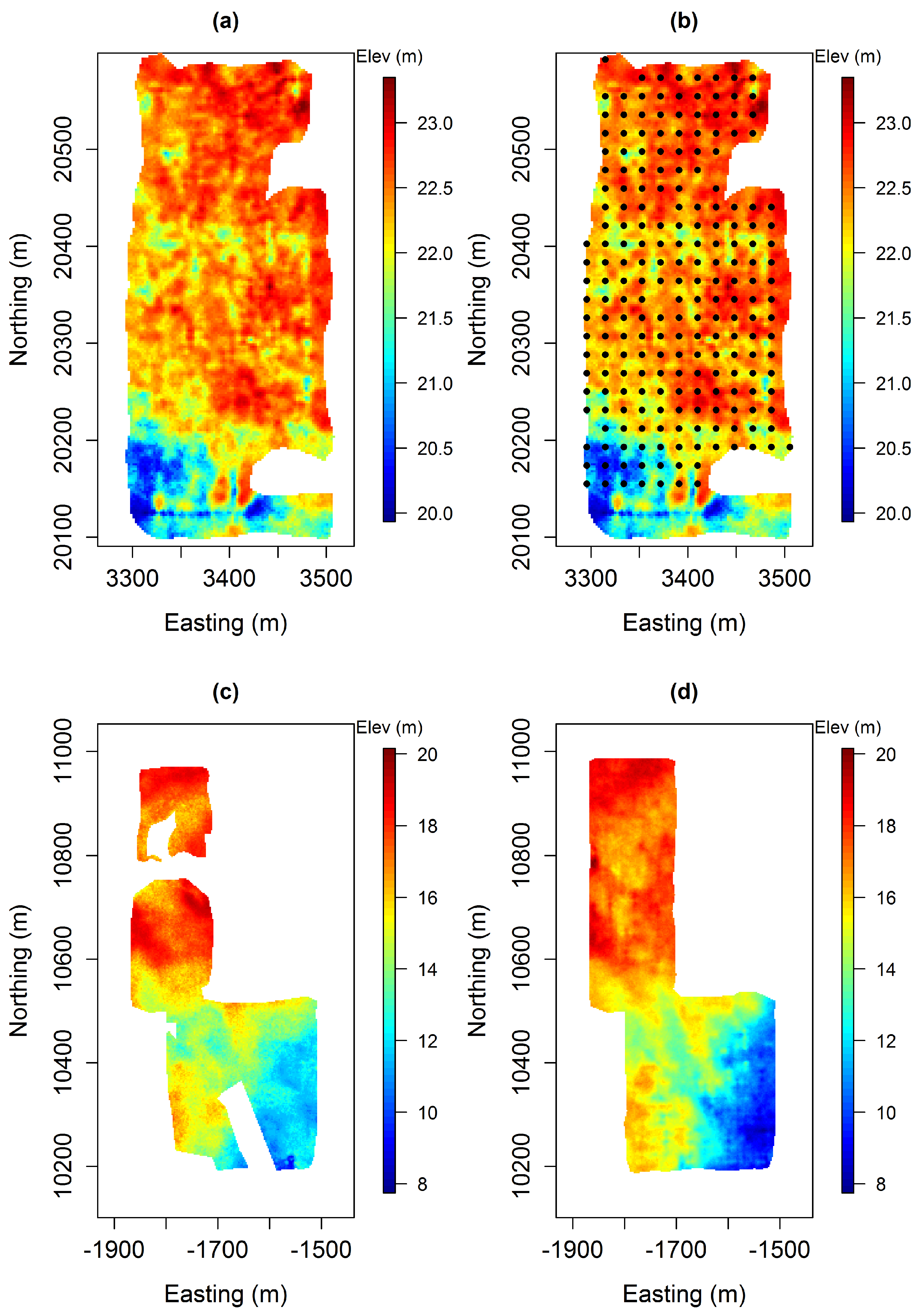
The data to perform the simulations comes from two mine sites. The first one (
Figure 1a,b) comprises a finite set of depth measurements collected from regularly spaced boreholes (conditioning data and primary variable) and an exhaustive Ground Penetrating Radar (GPR) survey (soft data and secondary variable). The position of the interface in this mine site is aimed to be simulated by DS, using these data sets as conditioning information. The second site is a mined-out analogue area providing a training data set. It includes the topographical survey of the exposed deposit base (primary variable) as well as a GPR survey done before the mining operation. This training data set, which is used as a bivariate training image, can be seen in
Figure 1.
In addition to this data, the simulation of the interface with DS requires the input parameters (number of neighbours, distance thresholds, etc.) to be determined. The aim of the proposed methodology is, therefore, to automatically obtain an optimal set of parameters for that purpose.
In lateritic bauxite deposits, the data sets may be dense and regularly organised. This offers the possibility to define a specific quality metric in which the patterns observed in the conditioning data can be taken as the target. Therefore, the general principle of the proposed methodology is to minimise an objective function representing the dissimilarity of the conditioning data with the simulated image in terms of pattern statistics. The calculation of the dissimilarity requires the pattern statistics to be computed. This is only done once for the conditioning data. For the simulated image, however, the pattern statistics change with each perturbation of the parameters and needs to be updated.
Methodology
The computation of the conditioning data pattern statistics first requires the migration of the borehole datapoints into the SG. This step is needed to convert the punctual data into the gridded type. Once this step is done, a search template
T is defined to retrieve the patterns contained in the borehole data. Since we are comparing the pseudo-histograms of one fully informed simulation image and a partially-informed borehole data image, a special search template needs to be constructed. Therefore, the construction of the search template
T is based on two parameters: (1) the number of grids between borehole data and (2) the number of borehole data desired to be used in one category of the pseudo-histogram. This is illustrated in the following example: say we have borehole data located in a grid at every five nodes in the x and y directions. If we want to capture a four boreholes data pattern, we choose the size of the search template to be 5 × 5. The constructed search template scans the borehole data grid and collects the patterns once four borehole data is captured by the search template. The collected patterns serve as the categories of the pseudo-histogram to be constructed. In order to account for the non-stationarity, the means
are subtracted from each
, focusing on the variation of each pattern around its mean. The steps mentioned above are illustrated in
Figure 2.
Following the construction of the smooth histogram categories for the conditioning data, the pseudo-histogram
for the conditioning data is computed by the following:
where
represents the number of patterns captured from the SG.
Once the smooth histogram of the borehole data is generated, the SA algorithm runs the DS algorithm to produce a realisation. The smooth histogram of this realisation is then computed using the categories created for the conditioning data histogram. In order to calculate the contribution of each pattern
in the histogram categories
, the means
are again subtracted from each
. The pseudo-histogram
of a realisation is calculated as follows:
where
is the number of patterns captured in the realisation image generated. Because there are more patterns in the simulation image than the conditioning data image, the weights in each category of the pseudo-histograms of the realisations are expected to be higher than those of the conditioning pseudo-histogram. In order to compare the pseudo-histograms, they are normalised before the computation of the Jensen–Shannon divergence. The normalisation is carried out through the following:
where
is the normalised weight corresponding to the weight of the
category
of either
or
. Subtraction of 1 from each individual pseudo-histogram category has been done to remove the weight contribution of each pattern
in its own
category. The Jensen-Shannon divergence is then calculated as follows:
Starting from an initial set of
DeeSse parameters (vector of decision variables), the SA algorithm runs the DS algorithm to produce a realisation and evaluate the objective function
. Then, the parameters are iteratively and randomly perturbed using the Cauchy-Lorentz visiting distribution. A new value of the objective function
is computed and the new set of parameters
is accepted or rejected according to a probability acquired from the generalised Metropolis algorithm. Factors influencing the probability of acceptance comprise the previous and candidate objective function values
as well as the number of iterations that have been made so far. During the initial iterations, the SA has a relatively high probability of accepting changes that may worsen the objective function. In order to explore the function that we want to minimise later in the process, this probability is reduced allowing the identification of the optimum better. The SA algorithm runs until the convergence is achieved and the objective function
O is minimised. The overall flowchart of the methodology is shown in
Figure 3.
The methodology was mainly implemented using R statistics software [
39]. The MPS simulations were performed by calling the DeeSse algorithm (which is coded in C) from R. For the optimisation part, we implemented the GSA using the GenSA package of R software [
40].
4. Results and Discussion
4.1. Implementation and Analysis of the Tuned Parameters on the Simulations
As explained in
Section 3, the aim is to model the lateral variability of the ore/waste contact surface in a lateritic bauxite deposit using borehole and GPR datasets (
Figure 1). For that purpose, we use a training dataset (bivariate TI) coming from an analogue site (
Figure 1c,d). The simulation grid has a size of 97 and 214 nodes in the
x and
y directions, respectively. The TI, on the other hand, is 180 × 400 in grid size. The spacing between the nodes of both the SG and the TI grids are 2.38 m. Since the data sets have apparent drifts, the types and the coefficients of these drifts were initially detected. First order trend surfaces for the TI and the second order trend surfaces for the simulation variables were found suitable and subtracted from the data sets to obtain the residuals. The residuals obtained were then used to perform the MPS simulations. Following the simulations, the trend surfaces were added back to each realisation.
Several combinations of DS parameters were initially tested to determine the appropriate simulation parameters by visually checking the simulation qualities. These initial attempts have shown that the simulation qualities were rather sensitive to changes in the parameter, making it difficult to identify optimal parameters through visually analysing the resulting simulations. The proposed methodology was then implemented. Five parameters that were considered during the optimisation procedure were
,
,
,
and
. The weighting factor
of the GPR data was not selected for the optimisation, as the simulation grid
of the GPR data was already exhaustively informed and any change in
would not affect the simulations. One of the main parameters of the DS algorithm, the scan fraction
f, was also not considered in the procedure. Based our previous trials, it did not affect the simulation quality significantly for this example. This observation of ours is rather consistent with the results presented in Meerschman et al. [
20]; they state that the parameter
f has a small effect on the simulation qualities unless it is below 0.2 for continuous simulations. Therefore, the scan fraction
f was kept equal to 0.5 throughout the optimisation procedure.
As the first step of our proposed algorithm, a search template is built to capture 4 points to construct the pseudo-histogram. Because the boreholes are drilled on a regular grid of 19.05 × 19.05 m and the grid spacing is 2.38 m, they are located in the SG at every 9th node in the x and y directions. Therefore, a 9 × 9 search template was constructed to capture four borehole data at a time. This search template was then used to construct the pseudo-histogram of the borehole patterns.
Having constructed the pseudo-histogram of the conditioning data, the SA algorithm was run with the following initial parameters:
= 10,
= 5,
= 20,
= 0.01 and
= 0.1. These parameters were selected as the ones yielding visually good simulation quality during the manual sensitivity analyses. In addition, the optimisation is also constrained by an upper and lower boundary, as can be seen in
Table 1. The resulting realisation is shown in
Figure 4a.
The pseudo-histogram
of the initial realisation is then calculated to compute the
mismatch. The JS divergence
between the pseudo-histograms
and
was initially calculated as 0.102. Using 30,000 function calls as the stopping criteria, the SA algorithm converged and found the parameters for the DS algorithm yielding a local minimum divergence value. The resulting realisation can be seen in
Figure 4b. The parameters along with their associated JS divergence values are provided in
Table 1.
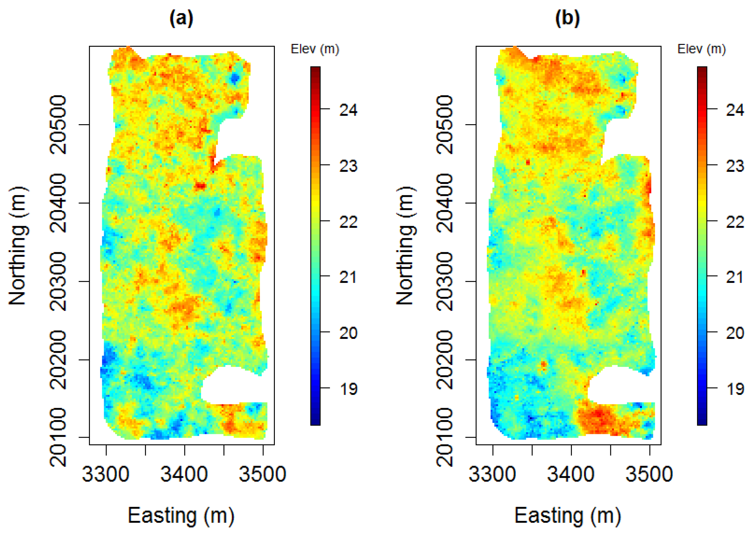
Although the initial and final realisations exhibit a noticeable difference, the average of 40 realisations generated using the initial and optimum parameters do not show an apparent dissimilarity, as can be seen in
Figure 5. However, the interquartile ranges of the elevation values calculated at each grid node noticeably dropped after the parameter tuning procedure, as illustrated in
Figure 5.
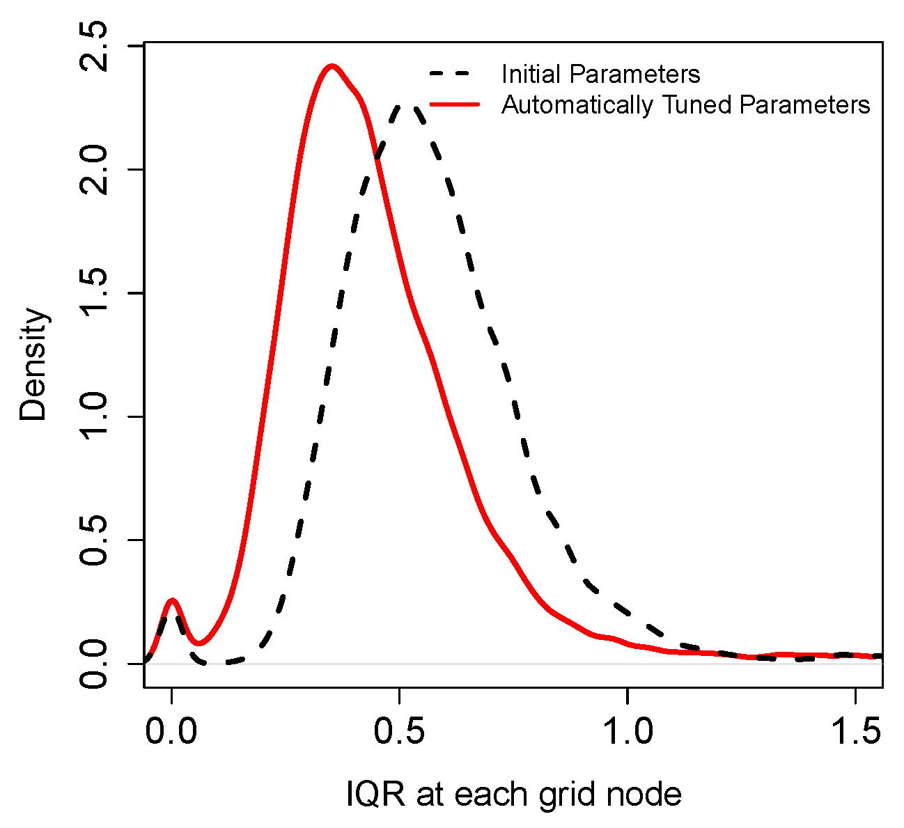
This can be seen more clearly in the distributions of IQR values shown in
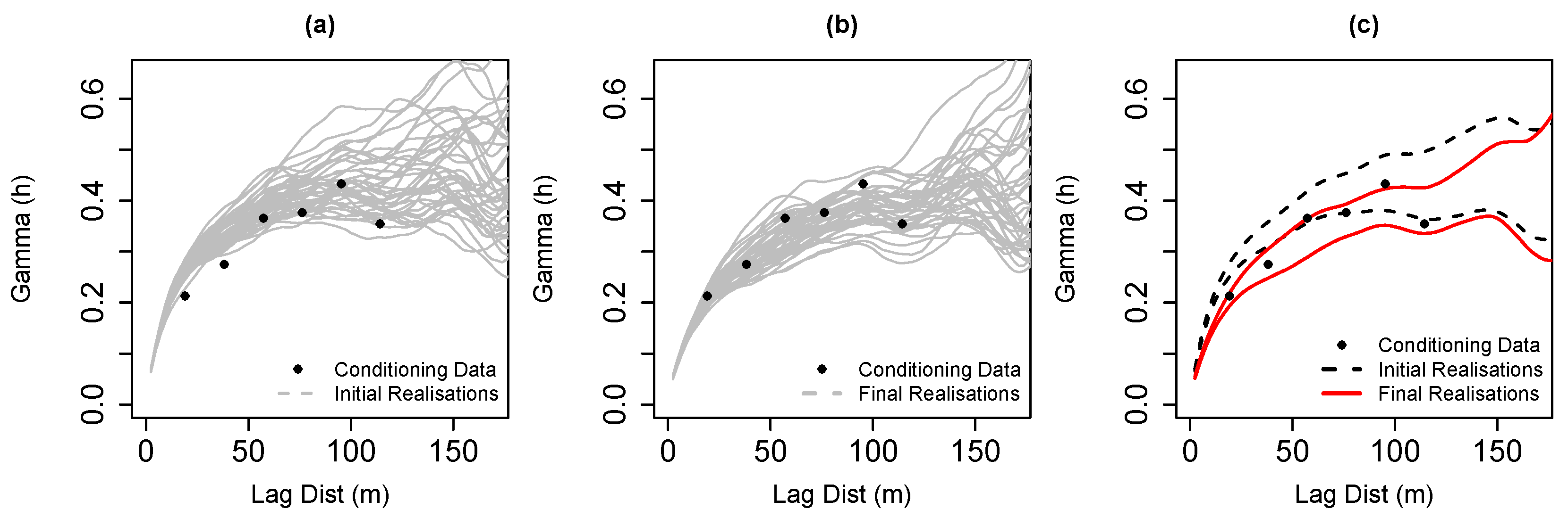
Figure 6. Similarly, the evolution of the variograms in
Figure 7 also shows that the variability between the realisations has decreased. In other words, the statistical fluctuations are better centred around the experimental variogram of the borehole data. These results indicate that although the means of the realisations exhibit a considerable similarity, there is a reduction in the estimated uncertainty around the mean. Since the optimised realisations are richer in terms of conditioning data patterns, the model of uncertainty would represent the original data variability better. Therefore, we consider the resulting uncertainty reduction as an improvement.
4.2. Effect of the Optimisation Method and the Initial Parameters on the Final Results
In order to test the choice of the SA, we compared the performances of different optimisation techniques. The parameter tuning process has also been carried out using other optimisation methods. These optimisers include the L-BFGS (quasi-newton type) [
41] and BOBYQA (trust region) [
42] methods. The optimisers were set to run with different initial parameters. These included a set of input parameters yielding a high JS divergence value, suggested parameters in Meerschman et al. [
20] and our initial parameters based on the manual sensitivity analysis.
The results in
Figure 8 indicate that the final value of the JS divergence is highly dependent on the initial parameters chosen for the BOBYQA and LBFGS optimisers. The performance of the SA algorithm, on the other hand, is less sensitive to the choice of initial parameters for these cases. Therefore, it is more robust and requires less preliminary manual sensitivity analysis. As discussed earlier, such a manual analysis is rather time consuming as it involves testing different set of parameters and observing the results manually. Furthermore, in three out of four cases, the SA outperformed the other optimisation algorithms in terms of reaching the minimum JS divergence.
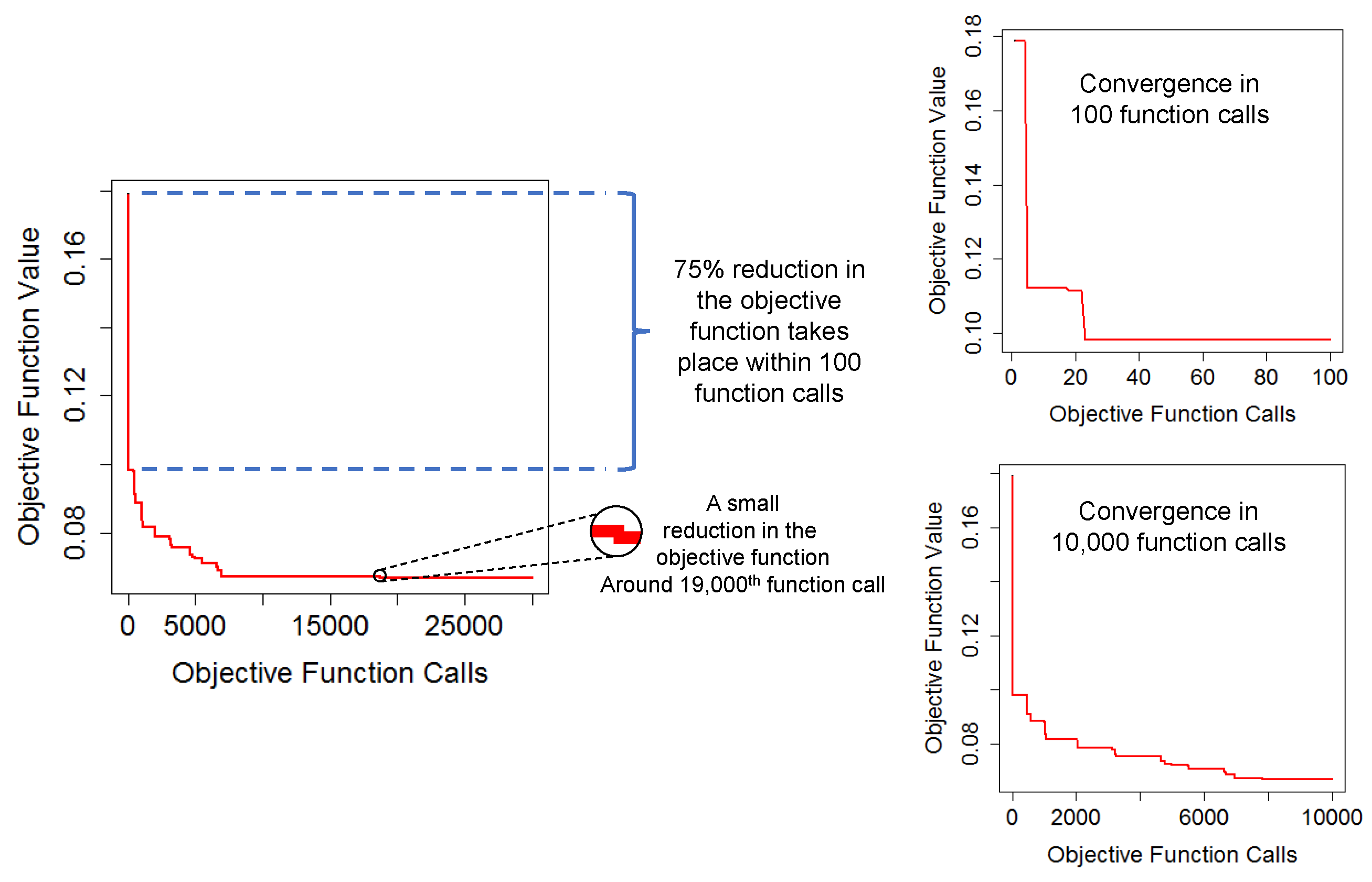
It should be noted that the optimizers used in this paper are reaching an optimum solution by utilising an iterative process. Hence, as the number of iterations increases, the probability of achieving a better solution increases as well. However, this would increase the total CPU time required for the optimisation. In the case study presented, 5 DS parameters were tuned to simulate the elevation values of the ore/waste interface. The simulation of 20,758 grid nodes took, on average, 4 s to perform one run using 8 threads. Using 30,000 simulations in the optimisation process, therefore, takes roughly 33.3 h to complete. If the method is applied for a problem with larger grid size, CPU time may become an important concern. Therefore, the number of iterations should be adjusted depending on the nature and the complexity of the simulations. Based on our experience obtained from this study, even 100 function calls with the SA seem to be adequate to find a better set of parameters than the visual inspection method. This can also be seen in the convergence plots of the SA for 30,000 function calls (
Figure 9). Taking the total reduction in 30,000 function calls as a reference (from 0.180 to 0.067), the graphs show that 75% of the reduction that is achieved actually takes place within 100 function calls. Whereas, 99% is achieved in 7000 function calls. Therefore, if feasible, the optimisation can be set to run around seven to eight thousand function calls. Otherwise, a hundred function calls would also yield satisfactory results.
4.3. Effect of the Chosen Parameters on the Pattern Reproduction
Since the JS divergence is a function of five DS parameters, the direct visualisation of its behaviour depending on the parameters is not straightforward. An approach to visualise such multi-dimensional problems is to plot the lowest JS divergence values in 1-D against individual parameters. This technique is called profile-likelihood and is utilised to check visually the parameters of a statistical model obtained via maximum likelihood techniques. The idea is to plot the maximum likelihood function values as a function of all but one parameter. It can also be considered analogous to tracking the maximum values along the crests of a five dimensional function. Given a model with parameters
and the likelihood
, the profile of the likelihood
for parameter
can be denoted as follows [
43]:
To create such 1-D profiles, 30,000 DS simulations were first performed. During these simulations, the tested parameters and their associated JS divergence values were recorded. In our case, we were interested in minimising the objective function. Therefore, we used the created data set to plot the individual parameters against the minimum JS divergence values.
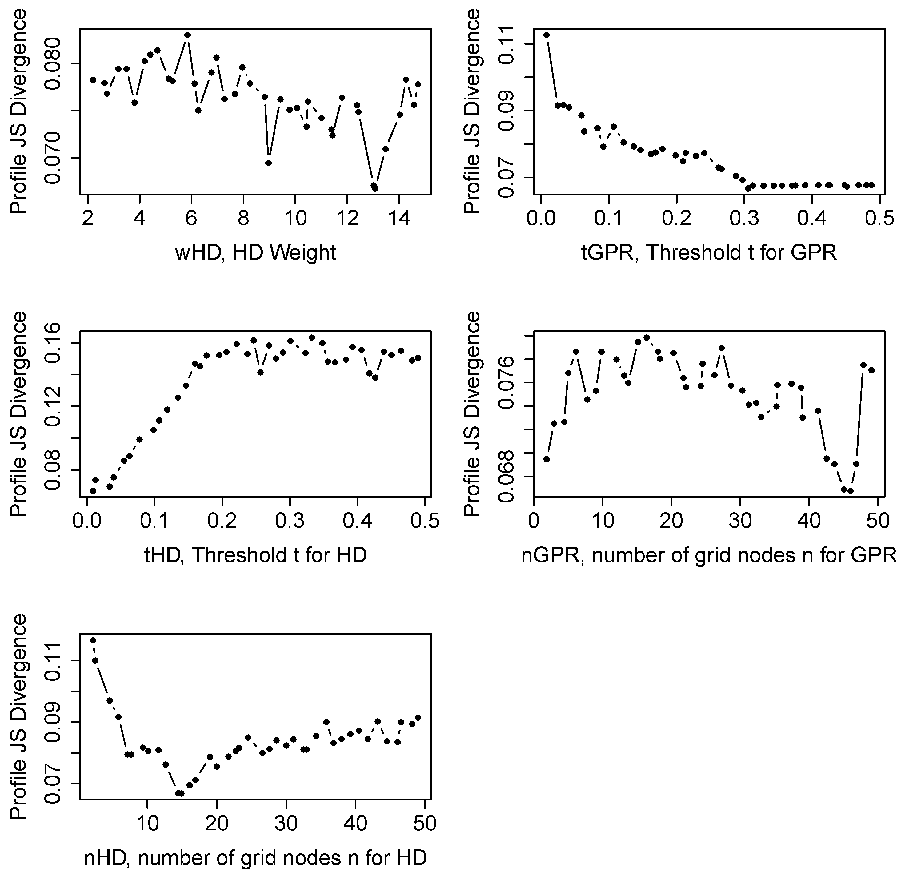
The created profiles shown in
Figure 10 help our understanding of the optimisation problem better and its sensitivity to the parameters. For instance, they show that as the parameter
increases, the JS divergence increases as well. This is an expected outcome as a high
would lead to poor reproduction of the conditioning patterns; hence, would yield a high JS divergence.
For the
parameter, the JS divergence decreases as expected with the maximum number of neighbours in the search template. But, the decrease stops at around thirteen and then starts to slightly increase with increasing
. It means that the conditioning data patterns are best reproduced with search templates consisting of approximately thirteen informed nodes. This is unusual since in most cases the patterns of the TI are better reproduced with more points [
20]. Here, the TI seems to contain features that are not present in the conditioning punctual data. One can see this as an indication that the TI is not fully compatible with the point data. But also, a very interesting feature is that the proposed automatic parameter identification is able to find automatically the best compromise between reproducing the patterns from the TI and those of the available point data. It is able to adapt the level of reproduction of the TI to ensure compatibility with the conditioning data.
Similarly, there is an apparent trend in the profile JS divergence for . As the increases, the JS divergence decreases and yields better simulation results. This is an unusual behaviour and can be better understood by being reminded of how the DS works. Considering a bivariate pattern collected from the SG, the grid nodes of the TI are visited to find a compatible match. During this search, a compatible pattern is considered to be the one with computed distances lower than the specified and . An increase in increases the probability of accepting a GPR component of the multivariate pattern as compatible. Therefore, the effect of the GPR variable becomes less pronounced in the simulations. Secondary information is normally considered to enhance the quality of the simulations. Here, the TI could be imperfectly compatible with the simulated area, as the multiple-point dependence between the reference mine and the simulation area could be different.
For the and parameters, the plots are noisy and do not exhibit a simple systematic decrease or increase. Considering that these plots were created using 30,000 simulation data, these noisy plots should not be due to insufficient data. A more likely cause could be the existence of many local minima. This could explain why the SA performed more efficiently than the other optimization methods.
Another observation is related to the sensitivity of the JS divergence to the parameters. When the range of the JS divergence values are considered, seems to be the most sensitive parameter as it has a high range of JS divergence values. This parameter is followed by and . The parameters and seem to have less effect on the resulting JS divergences. Another interesting observation is related to the and values. Both threshold values lose their significance on the JS divergence values above . Therefore, it can be concluded that the most influential range for these parameters for this case is between 0 and 0.3.
4.4. Analysis of the Automatically Tuned Parameters
The DS algorithm we used in this study was DeeSse. This version of the DS incorporates some modifications such as the introduction of a specific threshold for each variable rather than a global one as in the original version of Mariethoz et al. [
10]. Therefore, a direct comparison of the parameters we found with the parameters suggested by Meerschman et al. [
20] (based on the original DS) cannot be made. However, we can still get an insight into the parameters from their study. For instance, they have documented an increase in the pattern consistency by altering the conditioning data weight from 1 to 5. In our case, the optimal value was found to be 13.07. This means that high importance was given to the conditioning data points. Hence, better reproduction of the conditioning data pattern was attained. Also, the threshold value for a good quality simulation is suggested to be lower than 0.1 for the continuous variables. In addition,
is stated to produce noisy images. Our automatically found threshold values for the conditioning data, which is 0.009 is also consistent with their findings. However, GPR threshold
was determined as 0.305 and it is higher than their suggested values. The fact that
value is higher than
could be due to the objective function chosen. As the aim was to reproduce the conditioning data better in the simulations, the focus has automatically become more on better pattern consistency of the reference mined-out surface patterns.
5. Summary and Conclusions
In this paper, we presented a methodology to improve bauxite footwall contact simulations through an automatic parameter tuning process. The main idea was to identify the parameters best reproducing the patterns existing in the borehole/conditioning data. There are several benefits of relying on the borehole data patterns to tune the parameters. First, although the borehole data is a partial representation of the ground truth, they serve as precise and rather reliable information. Second, in lateritic bauxite deposits, the data set can be dense enough to compute the pattern statistics of the conditioning data as a reference to be targeted in the simulations. Third, getting a TI may sometimes be difficult. Considering the mined-out topography exposed after a bauxite extraction, the resulting surface might not be entirely compatible with the conditioning data of another area. Therefore, putting more emphasis on the conditioning data and borrowing the patterns from a TI can be considered as a merge between two sets of information. As a result, the adapted MPS parameters lead to generating realisations which contain the correct patterns observed at the location where the forecast is being made.
The proposed approach mainly provides three significant advantages. The first advantage is related to the uncertainty estimation. The evolution of the calculated IQR values at each grid node reveals a fair drop in the uncertainty after the parameter optimisation. Also, the observed convergence of the simulation variograms towards the conditioning data variogram indicates that the uncertainty estimation is more reliable after optimisation. Secondly, the parameter selection is carried out more objectively than with the usual trial and error approach. Identification of the appropriate parameters is performed based on an objective and quantitative criterion. Therefore, it naturally alleviates any subjective decision that can be made as a result of the visual inspection method. Third, the approach reduces the time and effort spent for the sensitivity analysis. Contrary to a traditional parameter tuning procedure in which a set of different parameters are tested and the results are analysed manually, the proposed approach selects the parameters automatically. This reduces the time and effort spent for the manual sensitivity analysis. Only some initial tests are required to set up the optimisation process.
In addition to the above-mentioned advantages, the selection of the pseudo-histograms of Melnikova et al. [
27] as pattern statistics provides: (1) the ability to calculate the pattern statistics of continuous images; (2) computation of the pattern statistics of regularly spaced borehole data and (3) an extensive flexibility when constructing the histogram categories. For instance, apart from the patterns of the borehole data, one can also include the patterns from the other sources to update the pattern categories. Examples of such sources may include the training images or simulations. All the patterns coming from different sources can then be used to construct the categories of the pseudo-histograms.
Visualisation of the behaviour of the JS divergence values based on the parameters has been performed through the profile-likelihood method. It allowed the analysis and better understanding of the behaviour of the objective function. The results have shown that the most influential parameters were , and . An interesting observation was made on . Contrary to the expectation, the JS divergence value increased with decreasing . Such a behaviour could be due to a possible TI compatibility issue and should be further investigated. In general, we believe that the observed objective function behaviours are related to both the choice of objective function as well as the case study. For instance, if the chosen objective function included the better reproduction of the TI patterns rather than the conditioning data, a different result could have been observed. Therefore, a different case study and the choice of the objective function could lead to a different behaviour.
One of the drawbacks of the proposed approach is the requirement of regularly spaced conditioning data to calculate the pattern statistics. We use the patterns with a particular spatial configuration in the pseudo-histogram construction. Therefore, the proposed method can only be used if the conditioning data is regularly spaced. Considering the stratified deposits such as lateritic bauxite, nickel or coal seams, a regularly spaced exploration borehole configuration is often implemented. Hence, the proposed approach can be used to aid parameter tuning for the MPS algorithms for such deposits. However, the conditioning data sets may sometimes be sparse and it may not be possible to accurately infer the multiple-point statistics of the conditioning data and make a comparison with the simulations. In such a case, the objective function could focus more on the reproduction of the multiple-point statistics of the training image and can easily be integrated into the objective function in the manner described in this paper.
The general workflow proposed in the paper could be adapted to irregularly spaced conditioning data, but this would require using a different quantification of pattern statistics. One idea could be to use cumulants [
8], because of the tolerances it offers for irregular grids. Another option would be to define a very different objective function focusing on a cross-validation approach where the quality criteria would be based on evaluating the MPS model performances. Most likely, the simulated annealing would still remain the most efficient algorithm to obtain the parameters since previous experiences have shown that the objective functions may contain local minima [
20].
Lastly, as this approach identifies the parameters iteratively, it requires computational time. This is a well-known feature of the SA technique. However, the strength of the approach is that it allows obtaining a global minimum even when the objective function contains many local minima. This has also been observed by the comparison made using different optimisers with different initial DS parameters. The SA does not get stuck in local minimum values as compared to the other methods. Moreover, when different the optimisations are initiated with initial input parameters, the SA appears to be the least sensitive method among the ones tested. Therefore, it might require less preliminary sensitivity analysis to define the initial parameters for the optimisations. These facts favour the use of the SA to tune the parameters automatically.


