Large-Scale 3D Modeling and Inversion of Multiphysics Airborne Geophysical Data: A Case Study from the Arabian Shield, Saudi Arabia

Abstract

Recent developments in large-scale geophysical inversions made it possible to invert the results of entire airborne geophysical surveys over large areas into 3D models of the subsurface. This paper presents the methods for and results of the interpretation of the data acquired by a multiphysics airborne geophysical survey in Saudi Arabia. The project involved the acquisition, processing, and interpretation of airborne electromagnetic, gravity, and magnetic geophysical data over an 8000 square kilometer area. All the collected data were carefully analyzed and inverted in 3D models of the corresponding physical properties of the subsurface, including 3D density, magnetization vector, and conductivity models. This paper summarizes the interpretation of all geophysical data sets collected during the field airborne survey. The goal of the paper is to demonstrate how the advanced 3D modeling and inversion methods can be effectively used for interpretation of multiphysics airborne survey data and to study and analyze the potential of the survey area for natural resource exploration in Saudi Arabia.

1. Introduction

Recent advances in system integration have enabled airborne geophysical systems to acquire simultaneously electromagnetic, gravity, and magnetic geophysical data, which can be interpreted for three-dimensional (3D) earth models relevant to groundwater, mineral, and hydrocarbon exploration. In the spring of 2016, the Saudi Arabian Glass Earth (pilot) project was conducted as a collaboration between TechnoImaging, King Abdulaziz City for Science & Technology (KACST), and Spectrem Air. The Glass Earth (pilot) project involved the acquisition, processing, and interpretation of airborne electromagnetic, gravity, and magnetic geophysical data over an initial 8000 square kilometer area of Saudi Arabia. The goal of the project was to study the top km of the Saudi Arabian landmass, so as to provide a road map for natural resource exploration in the survey area.

For interpretation of the multiphysics data collected by the airborne survey in Saudi Arabia, we have developed and applied advanced 3D forward modeling and inversion software, capable of modeling and inverting the data acquired over the entire airborne survey area. It is based on the concept of the moving sensitivity domain and large-scale parallel computing.

In this paper, we summarize the results of surveying and construct an integrated geological-geophysical model over the survey area (“Glass Earth Model”), which is based on the results of these inversions. We have also discussed correlations with geology and provide interpretations made from these data, including some recommendations of ground follow-up and further mineral exploration in the survey area.

Airborne geophysical surveying can economically cover large areas with the resolution required for mineral deposit exploration. These methods helped to discover hundreds of mineral deposits all over the world (e.g., [1]) Traditional interpretation of airborne geophysical surveys, e.g., magnetic and gravity, was based on the analysis of maps of the distribution of magnetic and gravity field data. Magnetic and gravity maps provide regional characterization of major geological features and can be useful in defining magnetic and density anomalies which may represent minerals associated with ore deposits (indirect or inferential detection). However, they alone cannot be used for identification of specific locations and types of mineral deposits.

In the case of airborne electromagnetic (AEM) surveys, simple techniques, like conductivity depth transforms [2] and 1D inversions (layered earth inversions, e.g., [3]), were used for interpretation of the airborne data. Advances are still being made with respect to these 1D methods to make them large scale and fast with parallelization (e.g., [4]). More advanced transforms have also been developed to extend the approximate inversion methods to 2D (e.g., [5]). Despite the advances, these methods will always be approximate and the development needs to be directed toward full 3D solutions (e.g., [6,7]).

To overcome the limitations of 1D inversions, several 3D inversion algorithms were introduced recently (e.g., [8,9,10]). These 3D inversion methods are based on more accurate modeling of the AEM fields; however, they still are difficult to apply to a large-scale airborne survey. These difficulties in performing full 3D inversion for airborne survey data stems from the necessity to solve the inverse problems for a large survey area. However, it is widely known that geophysical data are only sensitive to a limited sensitivity domain (e.g., [11,12,13]), which is significantly smaller than the area of even a small airborne survey. The sensitivity matrix for the entire 3D model can then be constructed as the superposition over the entire inverse model of the Fréchet derivatives from all corresponding sensitivity subdomains. This combined sensitivity matrix is much smaller (in an order of hundreds to thousands) than the sensitivity matrix for the entire modeling domain.

The concept of a moving sensitivity domain was introduced in [14,15,16,17]. This concept made possible a 3D inversion of frequency- and time-domain AEM data that did not rely on any approximations in the modeling or inversion kernels. Since then, others have also used this approach to introduce full 3D inversion codes based on finite difference [10], finite element [18] and hybrid FE-IE [19] solutions.

We applied advanced forward modeling and inversion software, based on the concept of the moving sensitivity domain, to multiphysics data collected by the airborne survey in Saudi Arabia. The developed “Glass Earth Model” presents the geophysical interpretations of the data collected by Spectrem Air during the 2016 airborne survey. Correlations with geology and interpretations are made from these data, including some recommendations of ground follow-up and further mineral exploration in the survey area.

The results of the Glass Earth (Pilot) project helped to identify a dozen potential mining targets, which can be associated with gold and other base metal deposits, including zinc and copper, potentially contained in Precambrian rocks of the Arabian Shield in the western part of the country. These targets typically have no surface expression, and can only be detected with modern high resolution geophysical methods as provided by the Glass Earth project.

2. Inversion Methodology

The general principles of modeling and inversion algorithms used in this paper are outlined in [20,21].

2.1. 3D Potential Field Modeling

Gravity (${\mathbf{d}}_g$) and magnetic (${\mathbf{d}}_H$) field data are linear with respect to the 3D density ($\rho$) and magnetization vector ($\mathbf{M}$) of the rocks. Therefore, the responses can be written in discrete form as follows:

$${\mathbf{d}}_g={\mathbf{A}}_g\rho ,$$

(1)

$${\mathbf{d}}_H={\mathbf{A}}_H\mathbf{M},$$

(2)

where ${\mathbf{d}}_g$ and ${\mathbf{d}}_H$ are $N_d$ length vectors of the observed gravity and magnetic field data; ${\mathbf{A}}_g$ and ${\mathbf{A}}_H$ are the gravity and magnetic operators, numerically expressed as the $N_d\times N_m$sensitivity matrices; and $\rho$ is the $N_m$ length vector of density and $\mathbf{M}=(M_x,M_y,M_z)$ is the $3N_m$ length vector of magnetization.

In the inversion, we use the measured response data ${\mathbf{d}}_g$ , ${\mathbf{d}}_H$ to recover the unknown density $\rho$ or magnetization vector $\mathbf{M}$.

2.1.1. Gravity Forward Modeling

The gravity field, produced by the density $\rho \left({\mathbf{r}}^{\prime }\right)$distributed within volume V of the rock, can be computed as the gradient of the gravity potential U:

$$\mathbf{g}\left(\mathbf{r}\right)=\nabla U\left(\mathbf{r}\right)=\gamma {\int \int \int }_D\rho \left({\mathbf{r}}^{\prime }\right)\frac{{\mathbf{r}}^{\prime }-\mathbf{r}}{{\left|{\mathbf{r}}^{\prime }-\mathbf{r}\right|}^3}dv,$$

(3)

where $\gamma$ is the gravitational constant and the gravity potential, $U,$ has the following form:

$$U\left(\mathbf{r}\right)=\gamma {\int \int \int }_D\frac{\rho \left({\mathbf{r}}^{\prime }\right)}{\left|{\mathbf{r}}^{\prime }-\mathbf{r}\right|}dv.$$

(4)

One can use the point-mass approximation to calculate Formula (3) in discretized form by considering each cell as a point mass [22].

2.1.2. Magnetic Forward Modeling

The anomalous magnetic field induced by the magnetic source distributed within volume V of the rock with the magnetization vector $\mathbf{I}\left(\mathbf{r}\right)$, can be represented by the following integral formula:

$$\Delta \mathbf{H}\left({\mathbf{r}}^{\prime }\right)={\nabla }^{\prime }{\int \int \int }_V\mathbf{I}\left(\mathbf{r}\right){\nabla }^{\prime }\left(\frac{1}{|\mathbf{r}-{\mathbf{r}}^{\prime }|}\right)dv,$$

(5)

where $\mathbf{r}$ is the radius vector of a point within the volume V; and ${\mathbf{r}}^{\prime }$ is the vector of an observation point. Most 3D magnetic inversion methods are based on the assumption that there is no remanent magnetization (e.g., [23,24]). However, the earth’s magnetic field is nonstationary over geological time, meaning that the direction of magnetization in a rock differs from the direction of today’s magnetic field. This effect is manifested by the presence of the remanent magnetization in the rocks. Under this assumption, we have to consider both induced and remanent magnetizations. To include the remanent magnetization in the magnetic field analysis, we introduce a magnetization vector, $\mathbf{M}$, which consists of two parts—induced, ${\mathbf{M}}_{ind}$, and remnant, ${\mathbf{M}}_{rem},$ magnetizations, respectively:

$$\mathbf{M}\left(\mathbf{r}\right)={\mathbf{M}}_{ind}\left(\mathbf{r}\right)+{\mathbf{M}}_{rem}\left(\mathbf{r}\right).$$

(6)

In this case, the intensity of magnetization, $\mathbf{I}\left(\mathbf{r}\right)$, is linearly related to the magnetization vector, $\mathbf{M}$, through the amplitude of an inducing magnetic field, $H_0,$ as follows:

$$\mathbf{I}\left(\mathbf{r}\right)=H_0\mathbf{M}\left(\mathbf{r}\right).$$

(7)

Thus, the anomalous magnetic field can be presented in the following form:

$$\Delta \mathbf{H}\left({\mathbf{r}}^{\prime }\right)=-H_0{\int \int \int }_V\frac{1}{|\mathbf{r}-{\mathbf{r}}^{\prime }{|}^3}\left[\mathbf{M}-\frac{3(\mathbf{M}·(\mathbf{r}-{\mathbf{r}}^{\prime }))(\mathbf{r}-{\mathbf{r}}^{\prime })}{|\mathbf{r}-{\mathbf{r}}^{\prime }{|}^2}\right]dv.$$

(8)

In the airborne magnetic survey, the total magnetic intensity (TMI) field is measured, which can be computed approximately as follows:

$$\Delta T\left({\mathbf{r}}^{\prime }\right)\approx \mathbf{l}\left({\mathbf{r}}^{\prime }\right)·\Delta \mathbf{H}\left({\mathbf{r}}^{\prime }\right)=$$

$$-H_0\mathbf{l}\left({\mathbf{r}}^{\prime }\right)·{\int \int \int }_V\frac{1}{|\mathbf{r}-{\mathbf{r}}^{\prime }{|}^3}\left[\mathbf{M}-\frac{3(\mathbf{M}·(\mathbf{r}-{\mathbf{r}}^{\prime }))(\mathbf{r}-{\mathbf{r}}^{\prime })}{|\mathbf{r}-{\mathbf{r}}^{\prime }{|}^2}\right]dv.$$

(9)

As in the case of the gravity field (Equation (3)), one can use the point-mass approximation to calculate the magnetic field in discretized form using Formula (9).

2.1.3. Modeling of AEM Data

Time-domain AEM modeling can be accomplished computing the EM field in the frequency domain and applying a cosine transform to the frequency-domain data [25]. For the Spectrem time domain data used in this paper, 31 logarithmically spaced frequencies from 1 Hz to 100 kHz were required to properly model the time domain response. As detailed in the inversion section, the parallelization is implemented over domains and data points, not over frequencies.

The conventional integral equation (IE) method of modeling the frequency-domain EM field is based on separation of the total EM field into the background, $\left\{{\mathbf{E}}^b,{\mathbf{H}}^b\right\},$and anomalous, $\left\{{\mathbf{E}}^a,{\mathbf{H}}^a\right\},$ parts as follows:

$$\mathbf{E}={\mathbf{E}}^b+{\mathbf{E}}^a,\mathbf{H}={\mathbf{H}}^b+{\mathbf{H}}^a,$$

(10)

where the background field is a field generated by the given sources in the model with a background distribution of conductivity, ${\sigma }_b$, and the anomalous field is produced by the anomalous conductivity distribution, $\Delta \sigma \left(\mathbf{r}\right)$, $\mathbf{r}\in D_a\subset R^3$.

Then, the electric and magnetic fields can be obtained by the following equations:

$$\begin{array}{c}\mathbf{E}\left({\mathbf{r}}^{\prime }\right)-{\mathbf{E}}^b\left({\mathbf{r}}^{\prime }\right)=\\ \underset{D_a}{\int \int \int }{\mathbf{G}}_E\left({\mathbf{r}}^{\prime },\mathbf{r}\right)\Delta \sigma \mathbf{E}\left(\mathbf{r}\right)\mathbf{dv}={\mathbf{G}}_E^{D_a}\left(\Delta \sigma \mathbf{E}\right),\end{array}$$

(11)

$$\begin{array}{c}\mathbf{H}\left({\mathbf{r}}^{\prime }\right)-{\mathbf{H}}^b\left({\mathbf{r}}^{\prime }\right)=\\ \underset{D_a}{\int \int \int }{\mathbf{G}}_H\left({\mathbf{r}}^{\prime },\mathbf{r}\right)\Delta \sigma \mathbf{E}\left(\mathbf{r}\right)\mathbf{dv}={\mathbf{G}}_H^{D_a}\left(\Delta \sigma \mathbf{E}\right),\end{array}$$

(12)

where ${\mathbf{G}}_E$ and ${\mathbf{G}}_H$ are the electric and magnetic Green’s tensors for a layered model with conductivity ${\sigma }_n$.

In Equations (11) and (12), the symbols ${\mathbf{G}}_E^{D_a}$ and ${\mathbf{G}}_H^{D_a}$ denote the electric and magnetic Green’s operators with a volume integration of $D_a,$ respectively.

The process of solving the forward electromagnetic problem according to Equations (11) and (12) consists of two parts. First, it is necessary to find the electric fields inside domain $D_a$ (where $\Delta \sigma \ne 0$), which requires the solution of an integral equation (domain equation) (11) for ${\mathbf{r}}^{\prime }\in D_a$. Second, using the data equations, (11) and (12), with ${\mathbf{r}}^{\prime }\in P$ , we calculate the electric and magnetic fields in the receiver’s domain P ([22,26,27]).

2.2. Geophysical Data Inversion

The inversion process is nonunique and unstable, therefore, one needs to use the methods of regularization theory to obtain a stable solution of the ill-posed inverse problem. We introduce parametric functional, $P\left(\mathbf{m}\right)$, as follows:

$$P^{\alpha }\left(\mathbf{m}\right)=\varphi \left(\mathbf{m}\right)+\alpha s\left(\mathbf{m}\right)\to min,$$

(13)

where $\varphi \left(\mathbf{m}\right)$ is the misfit; and $s\left(\mathbf{m}\right)$ is the stabilizing functional, respectively, and $\alpha$ is the regularization parameter [20,21].

We apply the re-weighted regularized conjugate gradient method (RRCG, [20]) to minimize the parametric functional $P^{\alpha }\left(\mathbf{m}\right)$. The re-weighting method converts the inversion problem into the space of weighted data and model parameters. The model weighting is based on the calculated sensitivities, which make the weighted sensitivities uniform across the model with respect to distance from measurement points. In its simplest form, this reduces to depth weighting. Data weights are also applied based on relative uncertainties in the data. The inversion runs until the misfit between the observed and predicted data reaches the noise level in the data.

An important distinguishing feature of our potential field’s inversion methods is the fact that the sensitivity matrix is computed on the fly and it is not stored in the computer memory. This approach dramatically reduces the memory requirements and speeds up the calculations; however, it also increases the amount of the computing power used for computations. To overcome this requirement, we employ the moving sensitivity domain approach. The concept of a moving sensitivity domain was introduced in [14,17]. This concept made possible a 3D inversion of airborne data that did not rely on any approximations in the modeling or inversion methods. There is no need to calculate the responses or sensitivities beyond the sensitivity domain. The sensitivity matrix for the entire 3D model can then be constructed as the superposition over the entire inverse model of the Fréchet derivatives for corresponding sensitivity subdomains. This combined sensitivity matrix can be stored as a sparse matrix with memory and computational requirements reduced by several orders of magnitude. We choose a sensitivity domain size such that the volume cells, which constitute typically between 95–99% of the total sensitivity are included in the receiver sensitivity domain. The radius of the sensitivity domain is dependent on the survey geometry and geology, but this survey was set to be 15 km for gravity and magnetic data, and 350 m for EM data. The radius is chosen through a combination of experience and gradually increasing the radius until the results no longer change with increasing distance. This makes the inversion results with the sensitivity domain virtually indistinguishable from those using the full 3D volume response.

To speed things up further on the CPUs, we precompute a neighbor list of the cell-receiver pairs that are within the sensitivity domain distance. As there are generally several orders of magnitude more cells than receivers and the cells are distributed horizontally across the MPI processes, it is more efficient to create the neighbor list for each cell, not each receiver.

The geophysical fields modeling and inversion is further sped up by domain based parallelization with both Message Passing Interface (MPI) and OpenMP and calculation of the numerical kernels on a graphics processing unit (GPUs). The MPI tasks are virtually independent which leads to nearly linear parallel scaling. A detailed analysis of the CPU time performance as a function of the number of processors can be found in [28]. The interested reader can find another example of large-scale gravity and magnetic field modeling in [29,30].

The AEM modeling and inversion are also parallelized with MPI and OpenMP. Due to the relatively high frequencies used in AEM, the moving sensitivity domain size is limited and as such modeling computation and storage requirements are relatively small for each data point. Furthermore, these requirements remain constant with increasing inversion domain size and amount of observation data. This allows us to primarily distribute the problem to MPI tasks over the data which are independent. Since we use the iterative solver, the number of iterations to solution can vary, which can lead to load imbalance. We alleviate this imbalance by round-robin distribution of the data points, as adjacent data points have similar characteristics leading to similar solver convergence [31].

3. Description of the Airborne Survey and Data Acquisition Systems

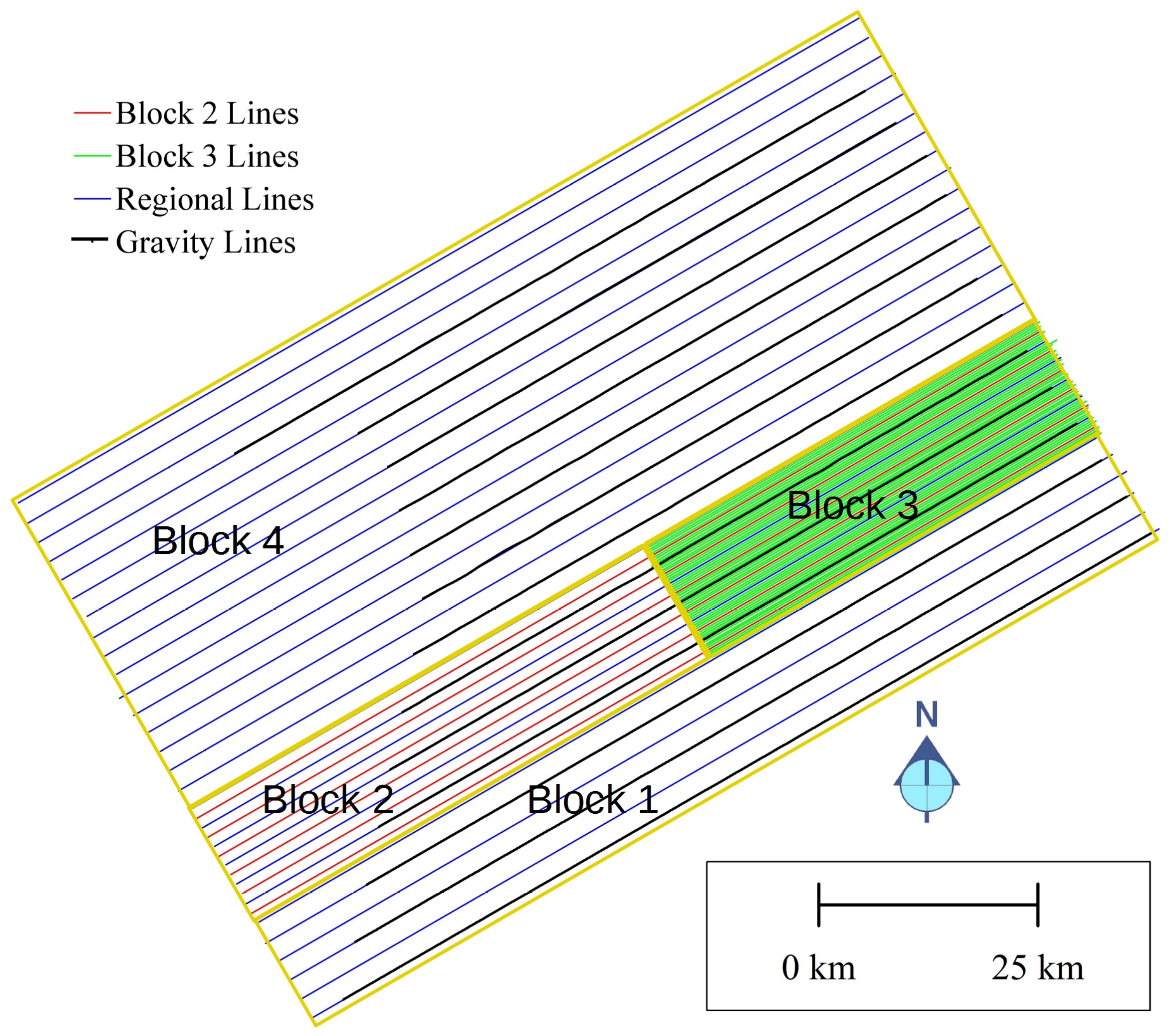
The airborne geophysical survey covered approximately 8000 km${}^2$ in the western part of Saudi Arabia. The survey area was divided into four blocks as shown in Figure 1. For the EM and magnetic data collection, we used three different line spacings to increase the resolution in some areas, while performing faster reconnaissance in other areas. The maximum line spacing was 2.5 km to give a high-level view of the geology, while other areas had a 1250 m or 250 m line spacing to increase the resolution and data coverage. The survey lines were designed to be flown perpendicular to the regional geologic strike. The regional survey was flown first. After analysis of this airborne data, sites within the survey area were back filled with 1250 and 250 m flight lines. All gravity lines were flown with 5 km line spacings.

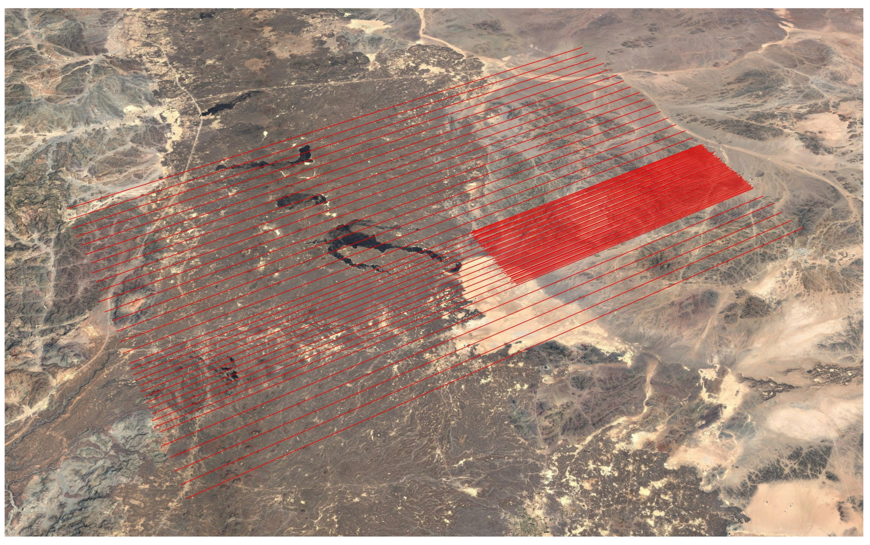
The selected area was first flown on a coarse grid, then back filled with denser survey lines which, based on the initial results, needed no changes from the initially planned locations (Figure 2).

The survey was performed by Spectrem Air, LTD, which is a fixed wing system. Airborne EM, gravity, and magnetic data were collected in the survey. These data types can be inverted to 3D models of density, electrical conductivity, magnetic permeability, and remnant magnetism to provide a comprehensive geophysical “look” at the earth’s surface and subsurface.

The Spectrem time domain system was used to collect the EM data. The transmitter was on the aircraft at a flight height of approximately 100 m, with the receiver 40 m below and 120 m behind the transmitter. Nine decays of the x, y, and z components were collected from the z-directed magnetic transmitter. The transmitting wave form was a 100% duty cycle square wave with a base frequency of 30 Hz. Collecting full duty cycle B-field data allowed for the best penetration possible.

We collected the total field magnetic data concurrently with the EM. The magnetic receiver was towed 19 m below and 41 m behind the plane. Magnetic measurements were made every few meters along the flight lines.

Approximately 1400 line-km of gravity data were collected. The flight height of the plane during the survey was fixed at 2200 m above sea level. The gravimeter was installed in the cabin of the plane. The instrument was a Micro-g LaCoste TAGS-6 gravity meter. Technicians from Scintrex installed and monitored the gravity data collection. Scintrex performed all the data processing in Saudi Arabia.

4. Geologic Background of the Survey Area

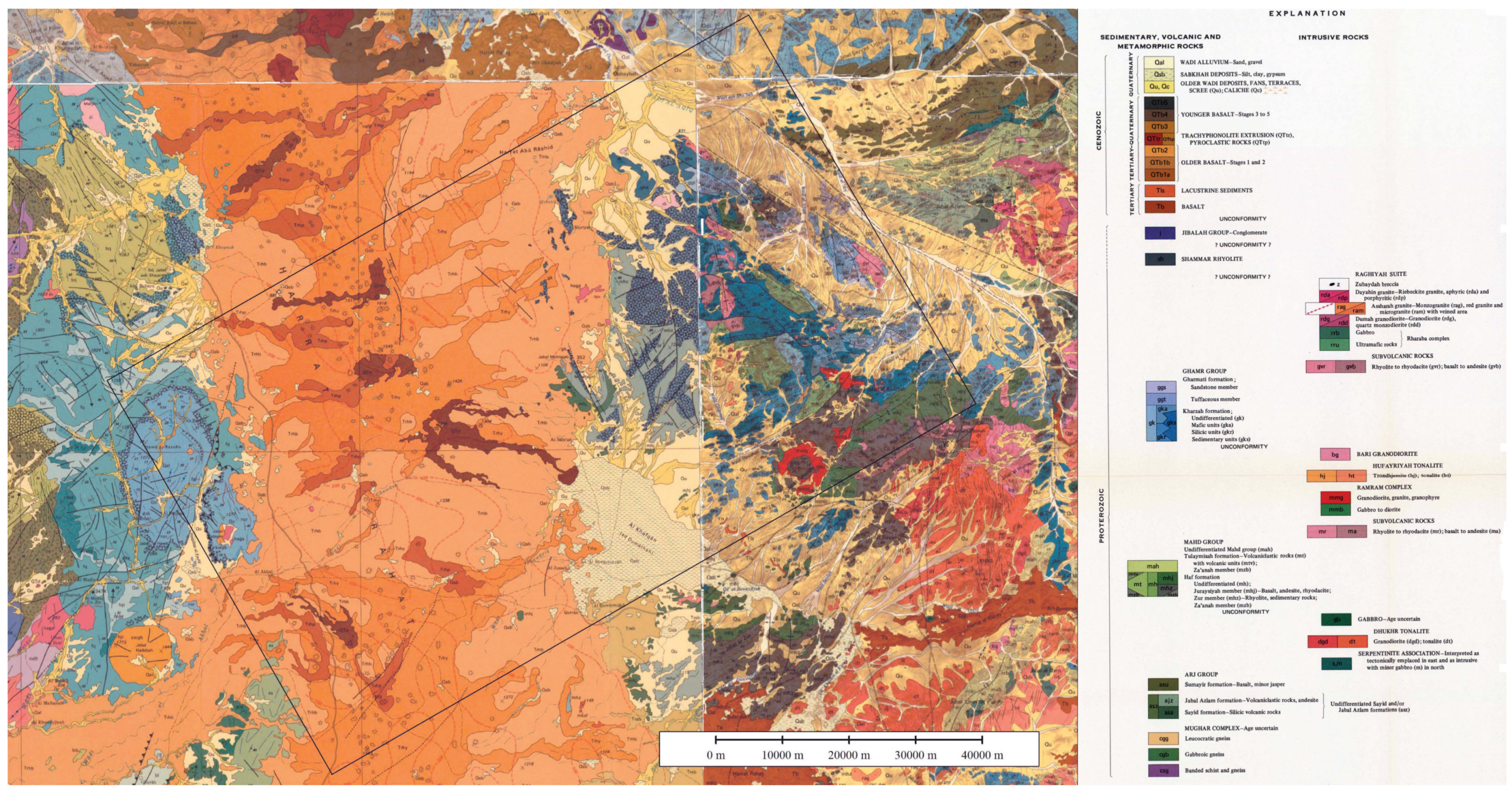
The survey area comprises three distinct geologic regimes. In the far west of the study area, the Precambrian Arabian Shield forms mountains up to nearly 1 km above the surrounding land. In the central part of the survey are Cenozoic volcanic rocks (harrats) that average several hundred meters in thickness, with a maximum thickness of around 400–700 m. They are very recent, with historic eruptions recorded in 1256 AD. These are underlain by the Arabian Shield. Approximately the eastern 1/3 of the survey area covers the Arabian Shield with sediment filled basins and mountains of locally high relief (100s m). The Quaternary sediments in the areas are predominately wadi alluvium, Aeolian sand and sand dunes, and terraced, slightly consolidated alluvium of old wadi deposits. These three provinces can be clearly seen in the geologic map shown in Figure 3.

The geologic map of the area shows several mineral occurrences in the Arabian Shield area in the eastern 1/3 of the survey area. Many of these were historic mines of archaeological interest, but little modern mineral extraction has occurred in the area. In addition, the active volcanism and proximity to the Red Sea rift zone brings the possibility of geothermal resources in the area.

5. Constructing 3D Earth Models

The multiphysics data collected by the airborne survey were used to create 3D models of different physical properties within the survey area (“Glass Earth” models). The inversions of geophysical data were done using the methods described above. In this section, we will discuss the main results of these inversions and present a brief description of corresponding 3D models.

5.1. Three-Dimensional Density Model

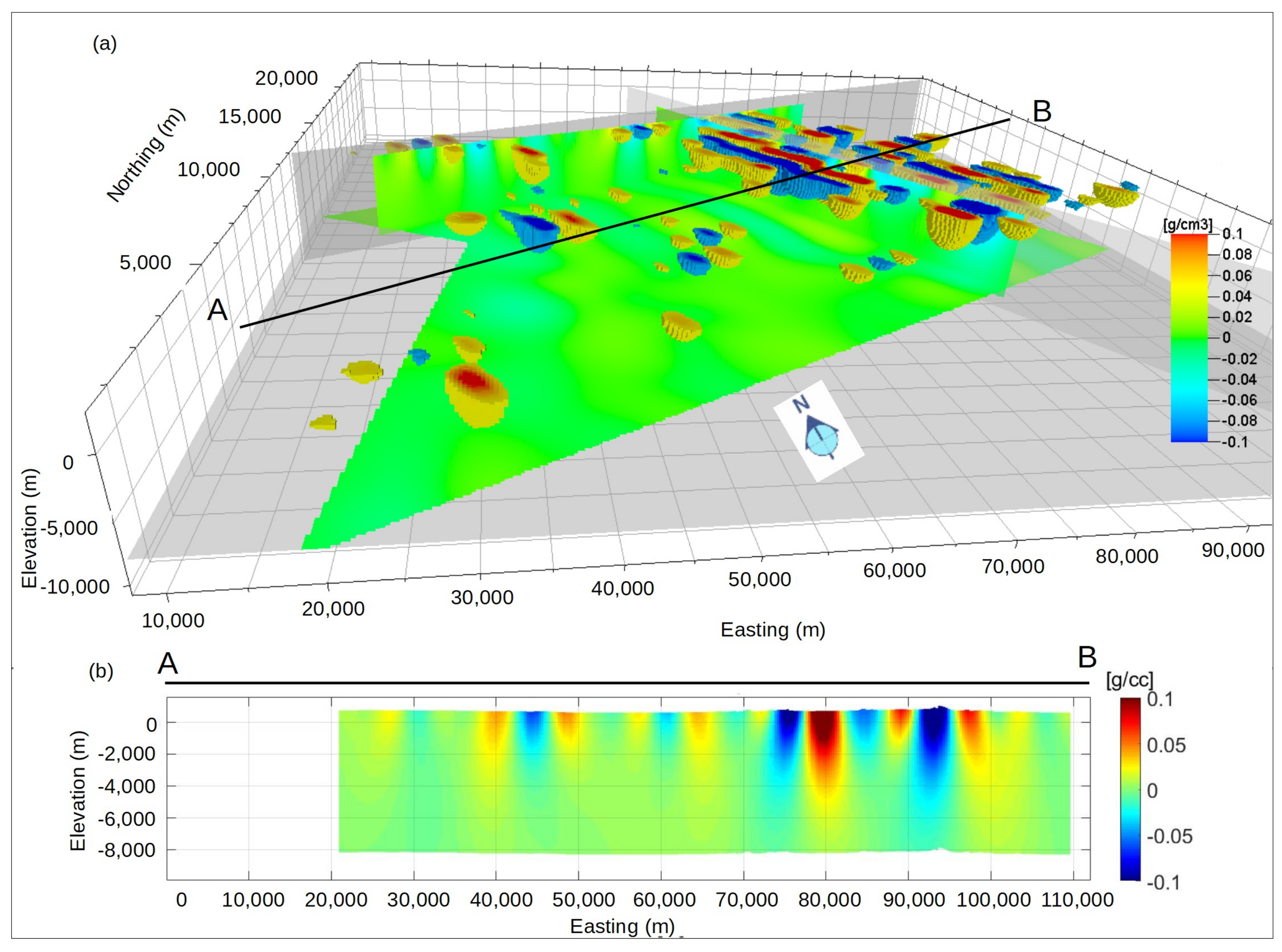
The Bouguer anomaly gravity data were collected by the airborne survey at 2200 m above sea level. These data were inverted on a horizontally uniform grid with 1000 m by 1000 m cell sizes in the x and y directions. In the vertical direction, the model grid increases logarithmically with depth and the vertical cell sizes vary from 175 m at the top of the model to 2900 m at the bottom. Forward modeling of gravity data accounts for topographic variations of the ground surface, so cells are adjusted in the vertical direction according to topography.

Figure 4 presents a perspective and cross-section view of the inverse density model. The color map indicates anomalous density. The hot colors indicate anomalously high densities, while the cool colors indicated anomalously low densities. The anomalous densities between −0.07 and 0.045 g/cm${}^3$ have been removed. This gives a transparent view of the anomalous materials— both positive and negative. The slices are also shown to give more depth and perspective to the model. The total thickness of the displayed section is 10,000 m.

A few larger regional anomalies are shown in the southwest, but most of the interesting features are in the eastern part of the survey. Overall, the regional trends in the density model show large, anomalous features in the eastern portion of the survey area. The lack of apparent density variations in and underneath the harrat is clearly shown in the figures.

5.2. Three-Dimensional Magnetic Property Model

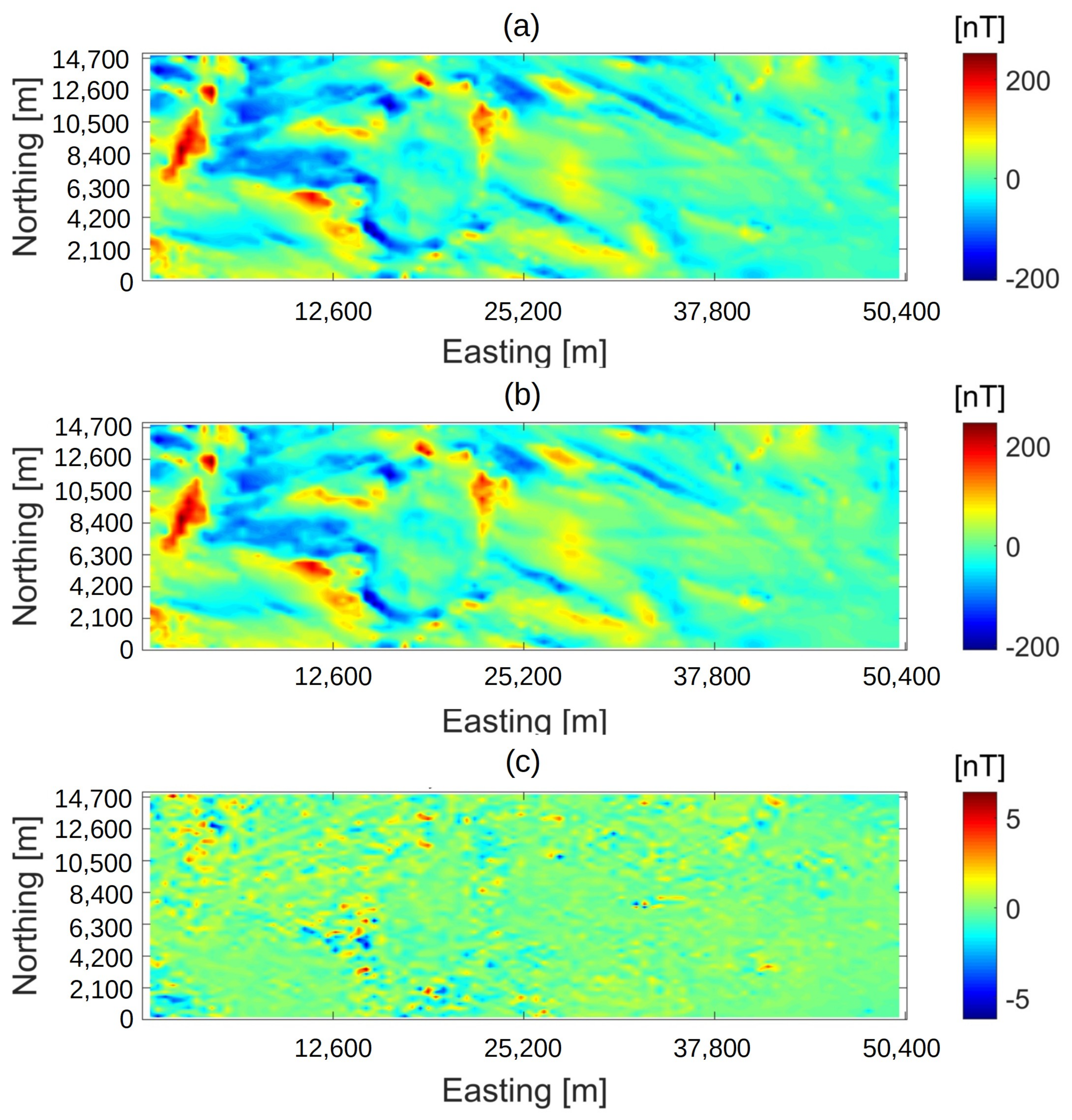
The inversions were run for the magnetization vector. We used filtered total magnetic intensity data in order to take into account the remanent magnetization (Figure 5, panel (a)). Block 3 was inverted on a grid that was 25 m in the in-line direction and 100 m in the cross-line direction. This inversion included leveled data from the Block 2 and regional flight lines. Block 2 and the regional survey were inverted with 100 m by 500 m cells in the in-line and cross-line directions, respectively. In all inversions, the vertical direction of the model grid increases logarithmically with depth and vertical cell sizes vary from 7.1 m at the top of the model to 129.4 m at the bottom of the model. Forward modeling of magnetic data accounts for topographic variations of the ground surface, so cells are adjusted in the vertical direction according to topography. A 10 km wavelength high-pass filter was applied to the observed data in order to increase the resolution of the near surface in the model. Each inversion converged to a normalized misfit of 2%. Panel (b) in Figure 5 shows predicted TMI data computed from the model of magnetization obtained by the 3D inversion. Figure 5c shows the final residual (predicted data subtracted from observed data). All areas have good data fit with no trouble spots.

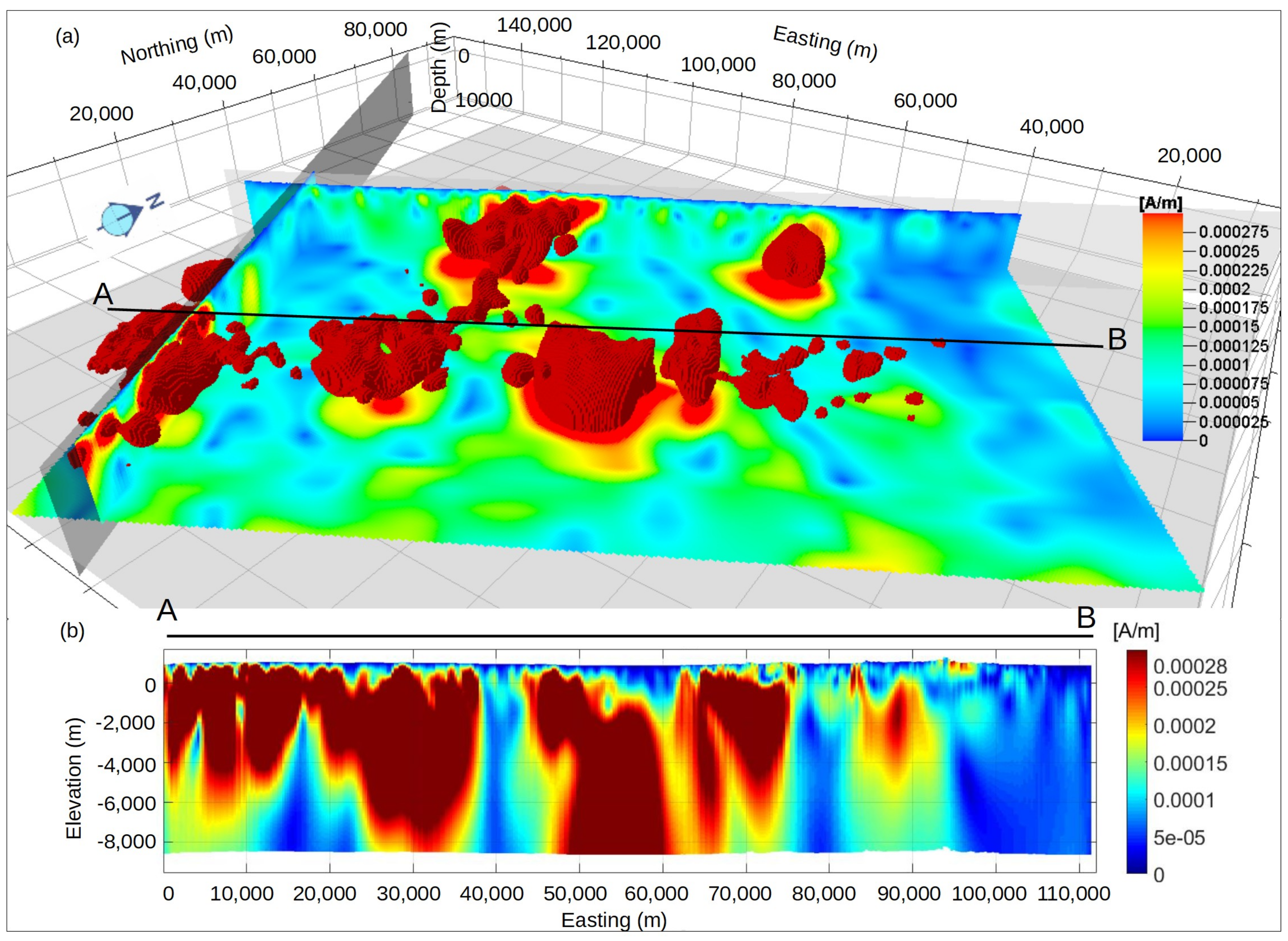
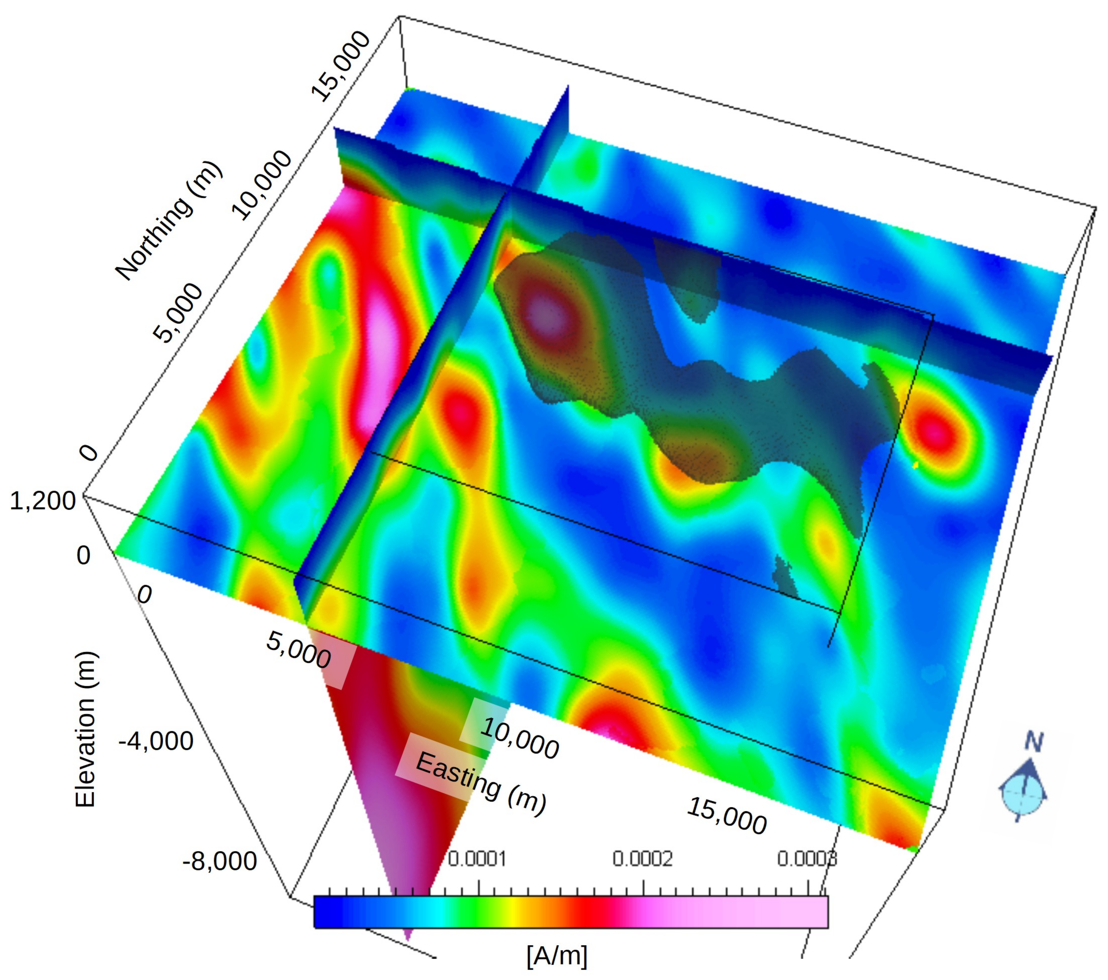
The final magnetic property model is shown in perspective and cross-section view in Figure 6. As with the gravity, the magnetic figures are shown in perspective view from the southwest to the northeast. The color bar corresponds to the magnitude of the magnetization vector. The hot colors indicate higher magnetization. Magnetization vector magnitude less than 0.000253 A/m has been removed from the volume for display, leaving only the anomalously high values. The slices are shown to help add perspective. The model is about 10,000 m in depth extent.

The different characters of the near-surface lava flows (shallow, stippled) are contrasted against the deeper-seated magnetic bodies, which extend to depth and are more coherent. These larger magnetic bodies are more likely to be associated with mineral or geothermal deposits.

5.3. Three-Dimensional Conductivity Model

All airborne EM data were inverted to 3D conductivity models using the technique described above. Many inversions were run using both 1D and 3D inversion codes to determine optimal parameters such as stabilizers, discretization, data error levels, and other regularization parameters. A 1D inversion was then run on the entire survey area to develop the background conductivity models and initial and reference models for the 3D inversion.

The area with closely spaced flight lines, Block B3, was inverted at 30 m horizontal cells in the in-line direction and 50 m in the cross-line direction. The model was divided into 16 cells in the z direction. The top of the first cell is the surface of the earth, and the bottom of the last cell is 1042 m below the surface of the earth. The cells varied in thickness from 10 m at the surface to 150 m thick in the deepest cell. A minimum norm stabilizer plus the 2nd derivative smooth stabilizer in the cross-line direction were used.

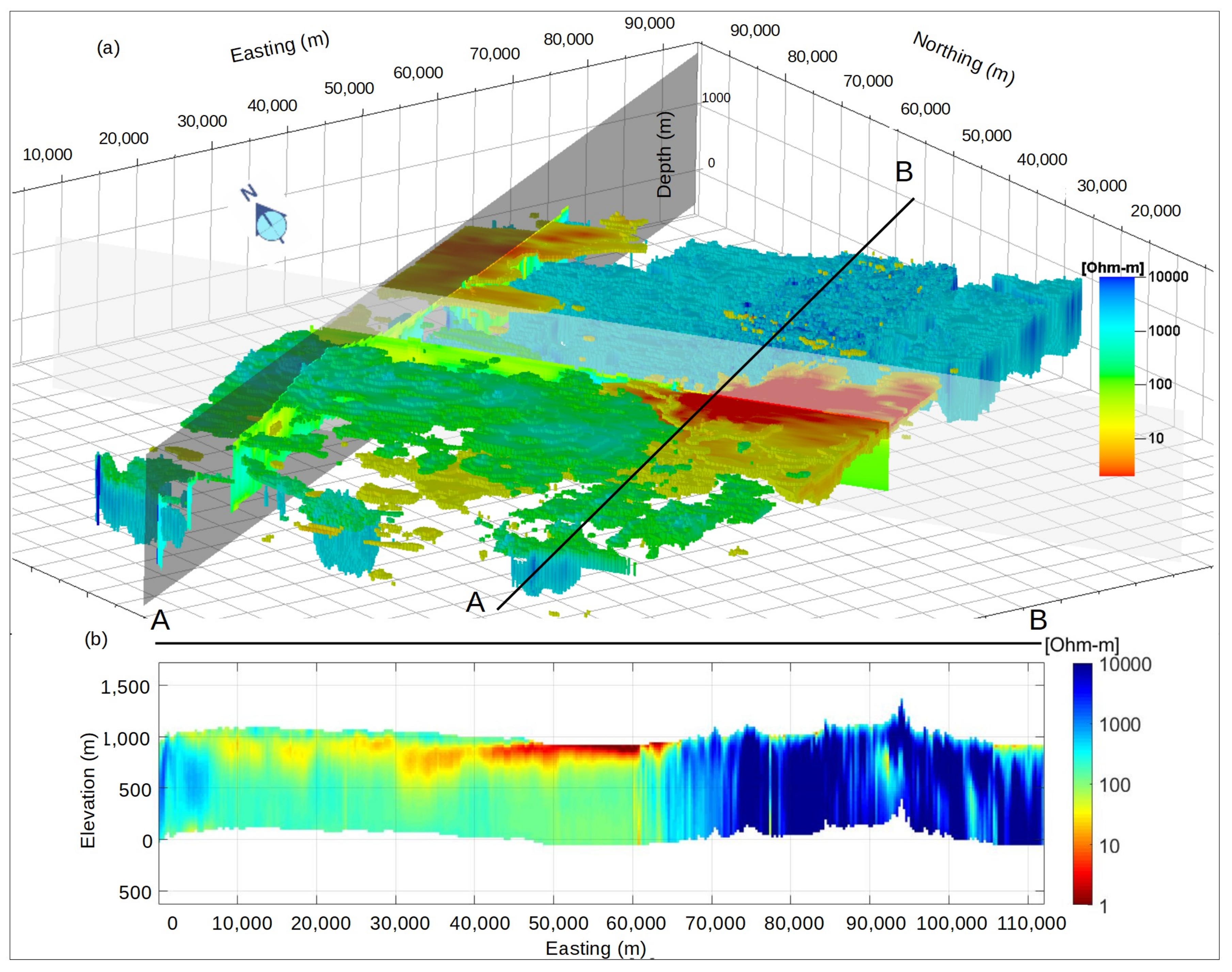
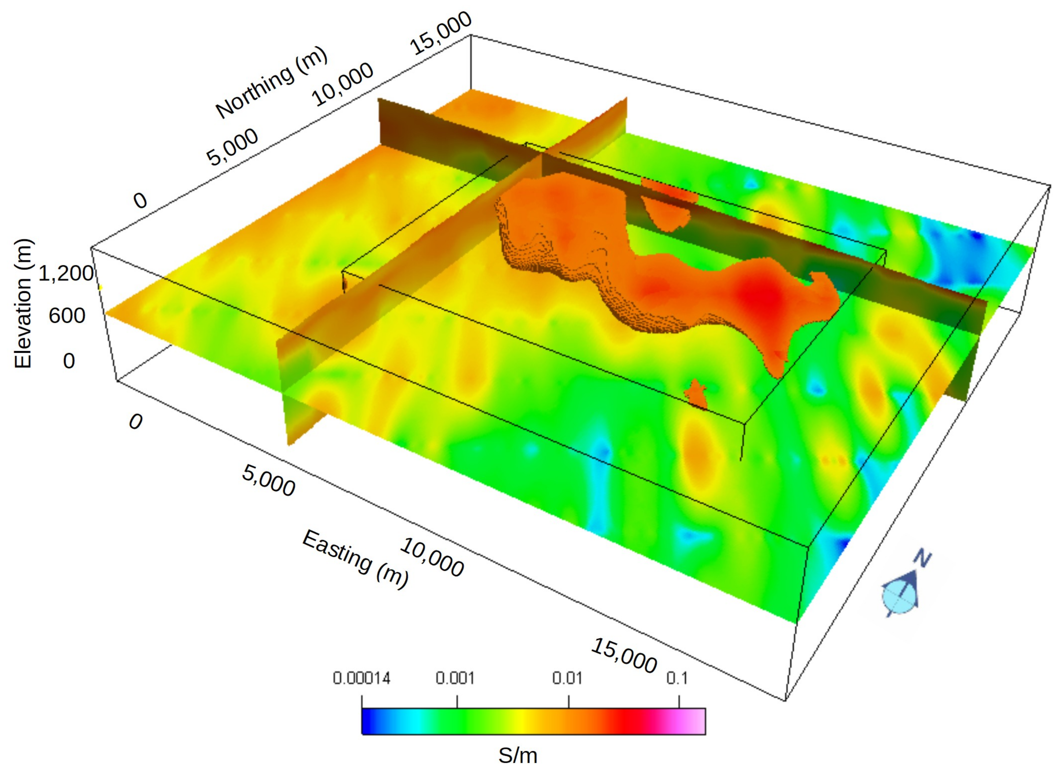
A regional view of the 3D conductivity model is shown in Figure 7. The model is shown in units of resistivity in Ohm-m. The total thickness of this model is 1900 m. The color map has been optimized to show several different terrains in the area. In general, the sedimentary basins, likely salt flats, are shown in red. The resistivity of these displayed values varies from 0.34 to 27.78 Ohm-m. The harrat in the center is shown in green, and the displayed values vary from 150 to 10,000 Ohm-m. The blue areas show the Arabian Shield with little to no conductive cover or lava flows. The displayed values in this area vary from 1300 to 10,000 Ohm-m. On the far side of the figure from this perspective is another section of conductive overburden from a sedimentary basin. This is less conductive than the southern basin.

Overall the conductivity model clearly shows several different terrains: the harrat, the exposed Arabian Shield, and two sedimentary basin areas with conductive overburden. The Arabian Shield has the most potential for near-surface mineral deposits that are clearly mapped with geophysics.

6. Glass Earth Model and Prospective Anomalous Targets for Mineral Resource Exploration

Bringing together the density, magnetization, and electrical conductivity data for the entire region provides a clear and comprehensive picture of the regional geology. In this section, we present an overview of the produced “Glass Earth Model” by highlighting regional features that correspond to the regional geology, but were previously unknown. We then list as an example several anomalies of interest which have mineral potential and should be targets for mineral resource exploration.

It should be noted that there is considerable potential for mineral and/or geothermal resources underneath the harrat (basalt flows), but these will be more difficult to explore, target, and drill than anomalies in the eastern region, where the shield is exposed. The eastern region contains the “low hanging fruit” in the survey area and it should be targeted first. When these targets are exhausted and more geologic information is gained, the exploration can then move outward, including under the basaltic cover.

6.1. Regional Structures

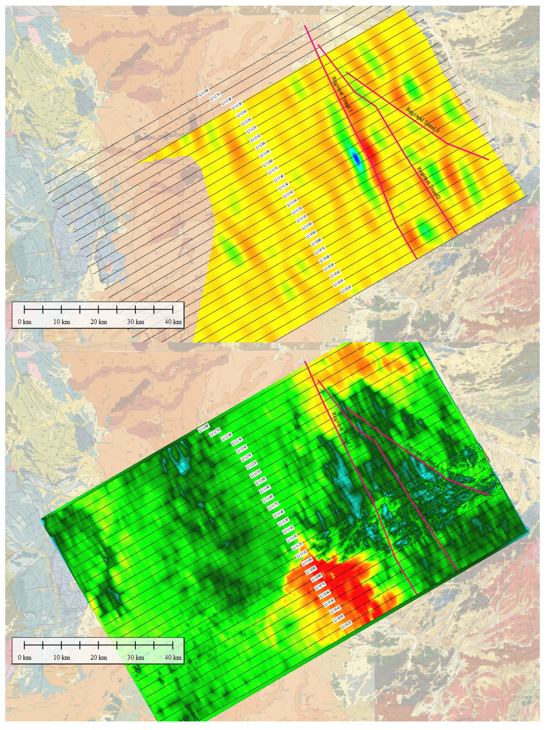
In general, the geology of the region has a NNW trend, paralleling the Red Sea rift zone. Many faults in the area are mapped with this orientation. The airborne gravity maps a large regional feature at 10 s of km depth, which is oriented almost directly NS and is centered on the edge of the harrat. This is also shown in Figure 8. The top panel in this figure shows the density variations in the top few 100 m. The hot colors are high density and the cool colors are low density. The bottom panel shows the electrical conductivity at the 100-m depth, with the hot colors showing higher conductivity. Both methods help map and reinforce the regional geology.

6.2. Local Anomalous Structures

Several anomalies of interest can be identified in the survey area based on the Glass Earth models of the physical properties of the subsurface. Note that the majority of the anomalies are located on or very close to the large regional features that have been identified. Exceptions are some anomalies that are on the mapped major structural feature (syncline), or on the inferred major fault.

While we can only speculate about the origin of these anomalies, the fact that both copper and gold mineralization is known in the surrounding area is very encouraging. Sulfides, such as pyrite, pyrrhotite, and chalcopyrite, are commonly associated with gold and copper mineralization. These minerals are electrically conductive and can often be detected by airborne surveys. We believe some of the following anomalies may be sourced from sulfides.

The area also has a large number of lava flows, some very recent. This is an indication of high heat flow in the area. The identified anomalies are of varied origin and are best suited for immediate follow-up. They give a good cross-section of the types of geophysical targets presented in the Glass Earth Model.

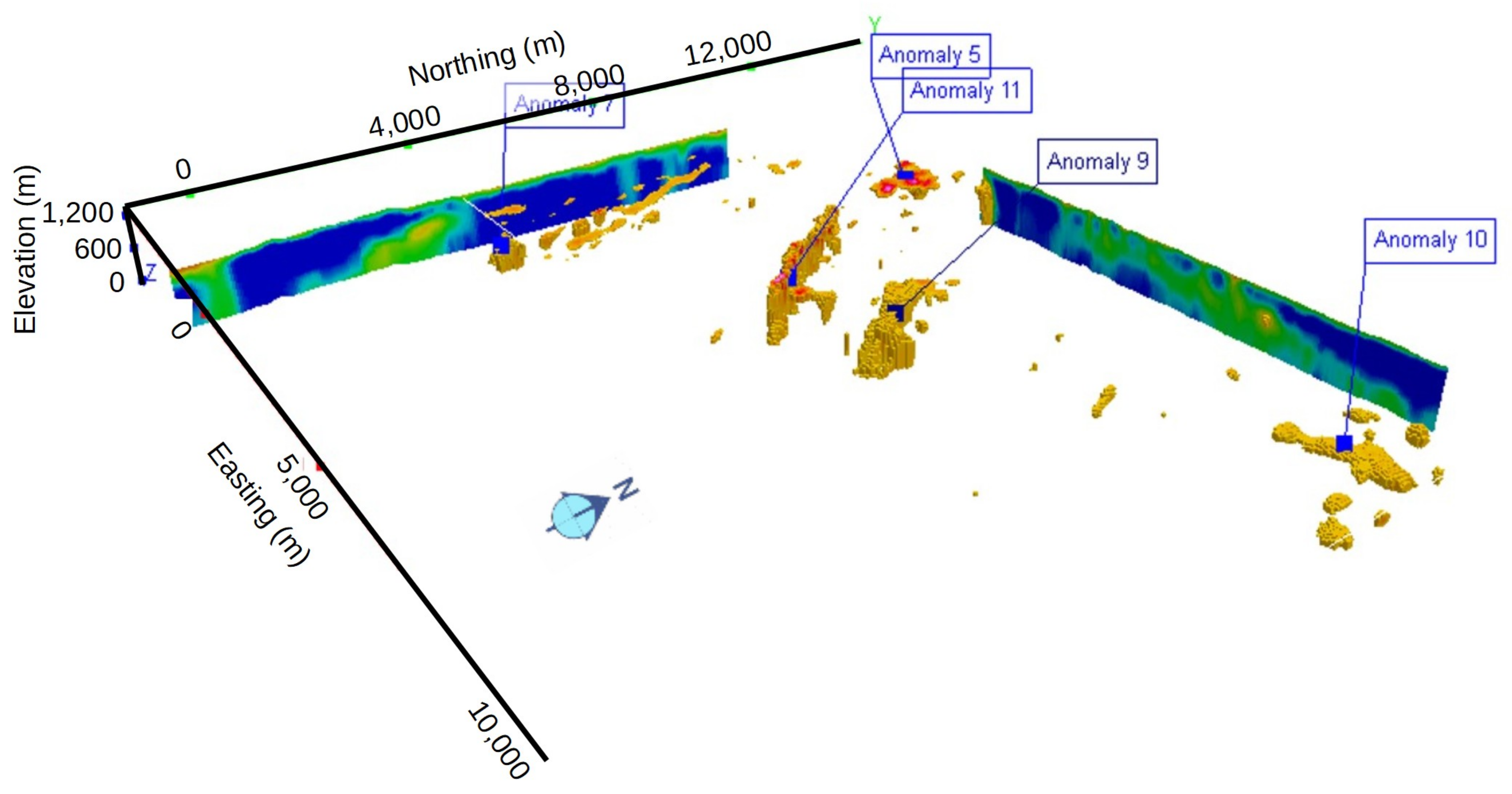
As an example, Figure 9 presents five anomalies shown based on the electrical conductivity, magnetic, and/or gravity responses. The airborne gravity data do not contain resolution to individually target these anomalies, but the area is in the large regional trend identified in the gravity anomaly. The image shows two vertical sections and also all voxels where the electrical conductivity is greater than 100 mS/m. The view is from the southeast. Anomaly 5 is primarily a conductivity anomaly which is flat laying and around 100 mS/m. Anomaly 7 is stronger (up to 1 S/m) and crosses four flight lines. It has a clear correlation with a large magnetic low associated with it and a magnetic high surrounding it. Anomaly 9 has conductivities exceeding 15 mS/m and is strongly correlated with a magnetic high. Anomaly 10 is a large (several square km) conductive anomaly exceeding 100 mS/m. It is flat laying, and does not have an associated magnetic response. Anomaly 11 is a near-vertical sheetlike conductor, with strong conductivities approaching 1000 mS/m and a coincident magnetic anomaly.

As an illustration, we present in the next figures the magnified images of one of the anomalous targets. This anomaly is associated with both a magnetic high and a conductivity high. The anomaly crosses two lines in this area of 2.5 km line spacing, which makes it relatively large and more certain of being representative of some specific geologic structure.

Figure 10 shows a 3D view of the local conductivity anomaly. The target is flat laying and moderately conductive. The view is to the southeast. Figure 11 presents both the conductivity and magnetic images of the same anomaly. The slices show the magnetic properties, while the cut-away shows the elevated conductivity. The magnetic highs can be seen to correspond to the electrical properties.

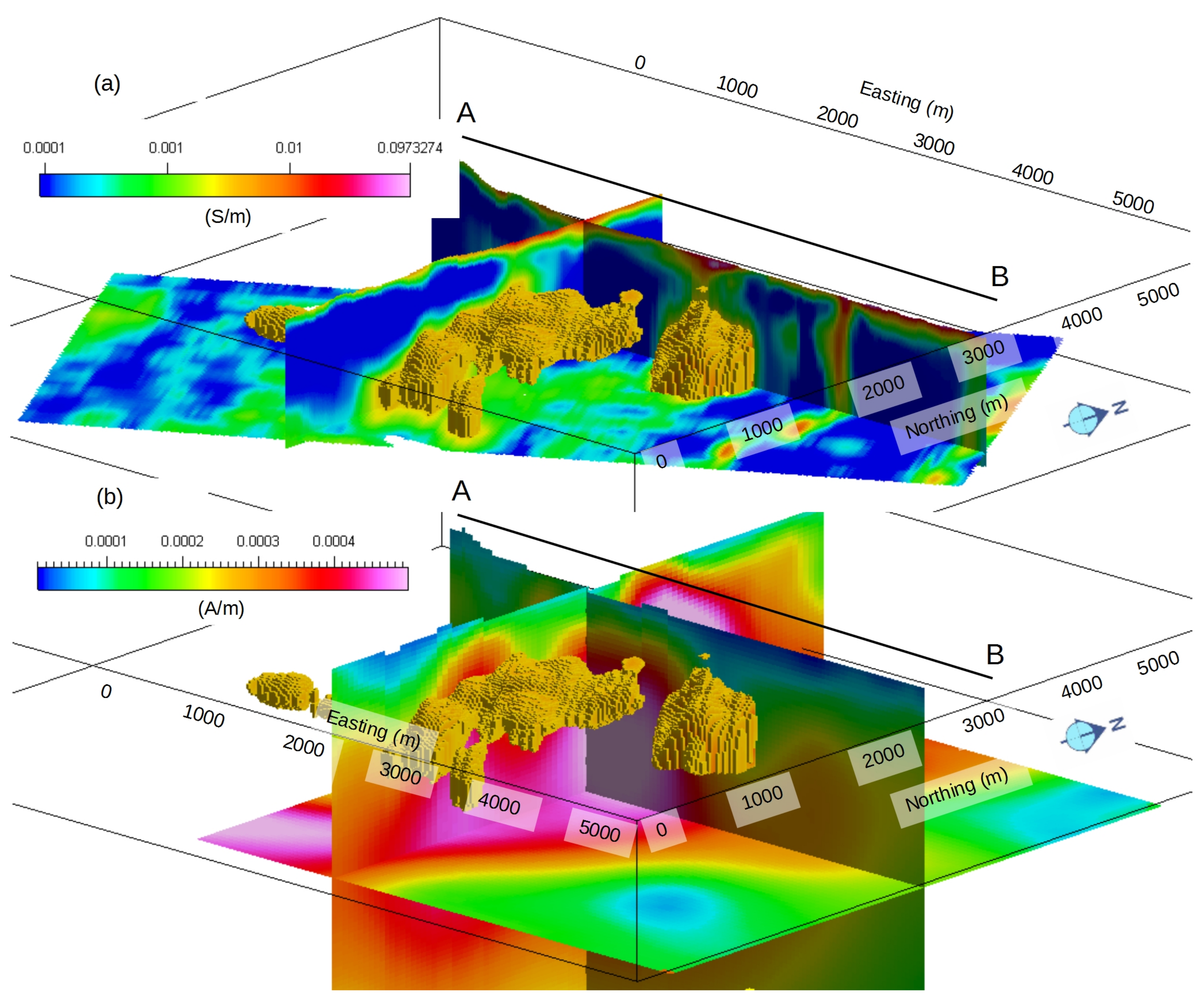
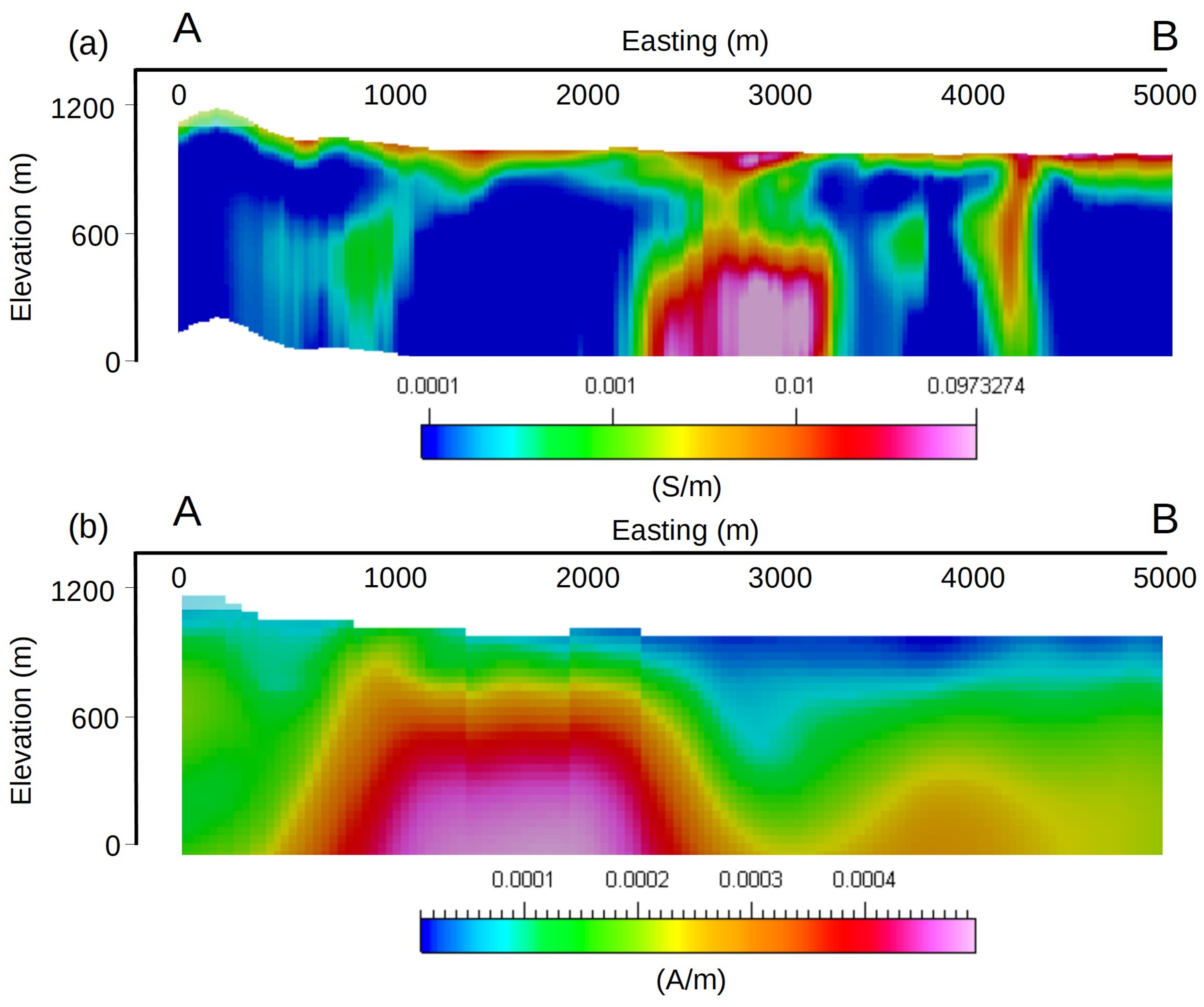
Figure 12 shows perspective views of another anomalous structure discovered by the Glass Earth survey. Panel (a) shows conductivity only, while panel (b) shows magnetic vector magnitude as the sections and conductivity as the voxels. There are two parts of the anomaly in this image: a north-eastern portion which is a large spheroidal body at depth, and a southwestern portion which is more tabular.

The southwestern portion has a clear dip to the southwest at about 25 degrees and extends for several hundred meters in depth. The conductivity of the feature is generally greater than 50 mS/m, while the host is less than 1 mS/m. The north-eastern part has higher conductivity (100–1000 mS/m), but is significantly deeper than the southwestern part. It extends to depth in the conductivity model (~800 m below the surface).

The body of the anomalous structure is associated with magnetics (Figure 13). Our interpretation is that the magnetic body shown in Figure 13 at 1500 m east is a resistive intrusion. The conductive feature nearby could be alteration due to the intrusion; it could contain disseminated sulfides, weathered bedrock, fractured bedrock altered to clay, or groundwater with clay or some amount of salinity.

7. Conclusions

We have developed an advanced 3D inversion method and software for 3D inversion of large-scale geophysical data collected by the airborne multiphysics system. This new data interpretation technology was applied to the airborne geophysical data collected over a survey area in the Arabian Shield in the framework of the Glass Earth (Pilot) project. The region selected for the Glass Earth project study has proven to be very productive from a geophysical standpoint. The area has interesting and diverse geology. It has significant mineral potential, as indicated by many mineralization zones shown nearby representative of gold, copper, and zinc. The proximity to recent lava flows and major structural features also makes this an area of interest for geothermal resources.

The area is relatively unexplored from a geophysical perspective. The potential geothermal and mining targets that exist and can be identified in the area, do not have any surface expression, and can only be detectable with modern high-resolution geophysical methods provided by the multiphysics airborne survey. Indeed, several targets have been identified for immediate follow-up. Currently, one of the anomalies shown here is undergoing further ground study based on these airborne analyses. The results of this study will be a follow-up paper. These targets may be associated with gold and other base metals, including zinc and copper, which are contained in Precambrian rocks of the Arabian Shield.

Note also in the conclusion that, joint inversion of multiple geophysical data could reduce the nonuniqueness and increase the robustness of the inversion. A joint inversion of the data collected in Saudi Arabia will be the focus of future research.