Provenance of Bengal Shelf Sediments: 1. Mineralogy and Geochemistry of Silt
by
 , ,
, ,
Laura Borromeo
1,* ,
,
Sergio Andò
1,
Christian France-Lanord
2,
Giovanni Coletti
1,
Annette Hahn
3 and
Eduardo Garzanti
1,* 1
Laboratory for Provenance Studies, Department of Earth and Environmental Sciences, University of Milano-Bicocca, 20126 Milano, Italy
2
Centre de Recherches Pétrographiques et Géochimiques, Université de Lorraine-CNRS, BP 20, 54501 Vandoeuvre-lès-Nancy, France
3
MARUM Center for Marine Environmental Sciences, University of Bremen, 28359 Bremen, Germany
*
Authors to whom correspondence should be addressed.
Minerals 2019, 9(10), 640; https://doi.org/10.3390/min9100640
Submission received: 30 May 2019
/
Revised: 23 September 2019
/
Accepted: 1 October 2019
/
Published: 18 October 2019
(This article belongs to the Special Issue Heavy Minerals: Methods & Case Histories)
Abstract
:This article illustrates a multi-technique frontier approach for the provenance study of silt-size sediments. The mineralogical composition of low-density and heavy-mineral fractions of four samples of fine to very coarse silt deposited on the Bengal shelf was analyzed separately for six different grain-size classes by combining grain counting under an optical microscope, Raman spectroscopy, and X-ray diffraction. The geochemical composition was determined on both bulk-sediment samples and on their <5-μm classes. Such a “multiple-window” approach allowed capturing the full mineralogical information contained in each sample, as well as the size-dependent intra-sample variability of all compositional parameters. The comparison between grain-size distributions obtained by different methods highlighted a notable fallacy of laser granulometry, which markedly overestimated the size of the finest mode represented by fine silt and clay. As a test case, we chose to investigate sediments of the Bengal shelf, where detritus is fed from the Meghna estuary, formed by the joint Ganga and Brahmaputra Rivers and representing the largest single entry point of sediment in the world’s oceans. The studied samples show the typical fingerprint of orogenic detritus produced by focused erosion of collision orogens. Bengal shelf silt is characterized by a feldspatho-quartzose (F-Q) composition with a Q/F ratio decreasing from 3.0 to 1.7 with increasing grain size, plagioclase prevailing over K-feldspar, and rich transparent-heavy-mineral assemblages including mainly amphibole with epidote, and minor garnet and pyroxene. Such a detrital signature compares very closely with Brahmaputra suspended load, but mineralogical and geochemical parameters, including the anomalous decrease of the Q/F ratio with increasing grain size, consistently indicate more significant Ganga contribution for cohesive fine silt. The accurate quantitative characterization of different size fractions of Bengal shelf sediments represents an essential step to allow comparison of compositional signatures characterizing different segments of this huge source-to-sink system, from fluvial and deltaic sediments of the Himalayan foreland basin and Bengal shelf to the Bengal Fan.
“Vast bamboo jungles towered over the river’s majestic banks, covering those muddy lowlands known to the world as the Sundarbans of the Ganges.”Emilio Salgari, The Two Tigers, Chapter 1.
1. Introduction
Silt represents a very major part of fluvial detrital fluxes and 50% or more of sedimentary covers on Earth [1,2,3,4]. Because of the diverse difficulties involved in sample treatment and analysis, however, mud and mudrocks are infrequently considered in provenance studies (e.g., [5,6]). Silt is a main component of offshore shelf deposits, which represent the trait-d’union between fluvial sediments largely carried in suspension and deep-sea-fan turbidites. Learning to extract provenance information routinely from silt-sized sediments, therefore, represents a major step forward in the understanding of the tectonic and erosional evolution of mountain belts.
The purpose of this article is to develop a standard procedure for provenance studies based on high-resolution analysis of silt-sized detrital minerals, choosing the Bengal shelf as a test case (Figure 1).
Himalayan-derived detritus is supplied to the Bengal shelf via the Meghna estuary of the Ganga and Brahmaputra rivers, which represents the largest single entry point of sediment in the world’s oceans [9,10]. Sediment is partly deposited on the shelf, and partly bypasses it to generate turbiditic currents feeding the largest submarine fan on our planet [11,12]. The thorough investigation of the mineralogical variability associated with hydrodynamic sorting and other physical and chemical processes in shallow-marine environments represents the fundamental pre-requisite to link the orogenic provenance signatures of Ganga–Brahmaputra sediments with the deep-sea sedimentary record [13,14,15,16]. This article and the companion paper dedicated to Bengal shelf sand [8] are, thus, intended as complementary to previous studies carried out on both bedload and suspended-load sediments of the Ganga and Brahmaputra rivers in the proximal part of the sediment-routing system [17,18,19,20,21,22,23,24,25,26,27].
In order to carry out a quantitative mineralogical study of silt samples with similar accuracy and precision as currently reached for sand, we coupled traditional optical analyses under a petrographic microscope with micro-Raman spectroscopy and X-ray diffraction. For each of four silt samples cored from the Bengal shelf, we separately investigated six different size classes (from <5 μm to >63 μm) obtained by wet sieving. Such a “multiple-window” approach allows capturing the full mineralogical information contained in the sample, as well as the size-dependent intra-sample variability of all compositional parameters [28,29]. The grain-size distribution and geochemical composition of the samples was also determined by diverse techniques.
2. The Bengal Sediment System
The Ganga and Brahmaputra Rivers form the greatest system of sediment transport on Earth [11]. The Ganga River drains the northern part of the Precambrian Indian shield with its sedimentary and basaltic (Deccan Traps) covers, and all tectonic units of the Himalayan belt. These include the Paleozoic to Eocene sedimentary succession of the Tethys Himalaya [30,31], mainly amphibolite-facies metamorphic rocks of the Greater Himalaya [32,33], lower-grade metamorphic rocks and sedimentary strata of the Lesser Himalaya [34,35], and foreland-basin siliciclastic rocks of the Sub-Himalaya [36,37]. In addition to the Himalayan belt, the Brahmaputra River drains granitoid batholiths and sedimentary covers of the Lhasa block [38], the Transhimalayan forearc-basin [39] and Yarlung Tsangpo ophiolitic suture [40], and high-grade metamorphic rocks of the eastern Himalayan syntaxis [41]. The syntaxis provides a large part of the Brahmaputra sediment load, whereas the Indo-Burman Ranges and the Shillong Plateau supply subordinate additional detritus in the lower course [20,21]. The Ganga and Brahmaputra Rivers join ~200 km upstream of the coastline to form the Padma River (the name of the Ganga in Bangladesh) and debouch into the Bengal Sea in the tide-dominated estuary called Lower Meghna, because it also represents the lowermost tract of the Meghna River draining the Shillong Plateau and the Tripura (Indo-Burman) fold-belt. To the west of the estuary lies the Sundarban mangrove forest, formed during progressive eastward migration of the Ganga outlet during the late Holocene [9,42].
At least one billion tons of siliciclastic detritus are produced annually by erosion of the active Himalayan range, and then funneled through the Meghna estuary into the Indian Ocean. Most commonly cited figures range from 380 to 480 × 106 t/a for the Ganga River and from 650 to 680 × 106 t/a for the Brahmaputra, which implies ~40% of the sediment flux from the Ganga and ~60% from the Brahmaputra [25,27,43].
Rapid erosion and transport continuing for several tens of million years ended up in the colossal accumulation of 12.5 × 10⁶ km3 of orogen-derived sediments in the Bengal Fan [44]. In the long term, only ~10% of Himalayan detritus remained stored in the Ganga foreland basin [45] without reaching the sea. Despite its smaller catchment (~0.6 × 10⁶ km2 vs. ~1 × 10⁶ km2), the Brahmaputra carries a larger sediment load than the Ganga [46], and it is the big-river basin with the highest denudation rate on Earth [47].
Ganga–Brahmaputra sediments reaching Bangladesh appear to be subequally partitioned among the delta plain, the prograding subaqueous delta, and the deep-sea fan [48]. The subaerial and submarine delta combined cover 138,000 km2, with total annual water and sediment fluxes from the Meghna estuary being around 970 km3 and 1.7 × 10⁶ t, respectively [49,50]. Most of the water and nearly all of the sediment are delivered during the summer monsoon season. Suspended load consists of fine to medium silt entrained close to the surface of the channel, passing to coarse and very coarse sandy silt at depth and to silty sand close to the channel bottom. Bedload is typically fine-grained well-sorted sand, and clay does not represent more than ~10%, even in surface load [19,25].
Offshore of the estuary mouth, a large subaqueous delta is prograding seaward. Wide sandy topsets extend down to water depths of ca. 15–30 m below sea level (b.s.l.) ~100 km from the coast, passing oceanward to delta-front foresets and beyond, at water depths around 80 m b.s.l., to muddy prodelta bottomsets [51,52,53].
2.1. Mineralogy of River Silt
Silt carried by the Ganga and Brahmaputra Rivers contains quartz and mica in similar proportions, associated with feldspar and heavy minerals. Quartz, feldspar, and heavy minerals steadily increase from shallow to deep suspended load relative to phyllosilicates. Composition, thus, changes from mica > quartz > feldspar in shallow suspended load to quartz > feldspar > mica close to the riverbed. The Ganga carries more quartz and less Ca-bearing plagioclase than the Brahmaputra. Ganga suspended load contains significant calcite and dolomite, and a moderately rich epidote–amphibole–garnet suite including clinopyroxene, tourmaline, titanite, rutile, zircon, kyanite, apatite, sillimanite, staurolite, and chloritoid; garnet increases progressively with depth relative to less dense amphibole and epidote. Brahmaputra suspended load contains virtually no calcite, very little dolomite, and a rich amphibole–epidote suite including garnet, clinopyroxene, minor titanite, tourmaline, apatite, rutile, sillimanite, zircon, kyanite, chloritoid, staurolite, hypersthene, monazite, and Cr-spinel [24].
2.2. Geochemistry of River Silt
Differences in the chemical composition of suspended load carried by the Ganga and Brahmaputra Rivers are difficult to determine accurately because of strong grain-size control. For a given grain size, Brahmaputra sediments are richer in Na, Sr, Cr, P, and possibly Co and Ni, reflecting higher abundance of plagioclase, amphibole, apatite, and Cr-spinel. Ganga sediments are instead richer in Ca, reflecting more abundant carbonate grains. Fine silt entrained close to the surface is strongly enriched in mica, clay minerals, oxy-hydroxides, and organic matter, and it is consequently characterized by higher concentration in chemical elements hosted in phyllosilicates, in heavy metals adsorbed on clays, and in constitutive water (Al, Fe, Mg, K, Ti, P, Mn, Rb, Cs, Be, Ba, V, Cr, Mo, W, Co, Ni, Cu, Zn, Ga, Ge, Pb, As, Sb, and Bi). Instead, because of progressive enrichment in faster-settling coarser, denser, and more spherical grains toward the bed, elements mostly hosted in tectosilicates (Si, Na, Ca, Sr) or ultradense minerals (Zr, Hf) are concentrated in deep suspended load. Other elements hosted in ultradense minerals but also associated with fine particles (Y, REE, Th, U, Ti, Nb, Ta, Cr, W, Mn, Fe, Cd, Ge, Sn, and P) reach maximum abundance in deepest suspended load, particularly above heavy-mineral-rich bedload, but are also enriched in surface load [19,24,25,27].
2.3. Clay Minerals
Because of high rates of physical erosion in the Himalayan orogen, the clay–mineral assemblage carried by the Ganga and Brahmaputra rivers is dominated by illite, with subordinate chlorite, smectite/montmorillonite, and kaolinite. Notable differences occur between Ganga and Brahmaputra clays. Because storage time and weathering intensity is notably higher in the Ganga than in the Brahmaputra floodplain [26,54], and because southern Ganga tributaries such as the Chambal River drain the Indian shield capped by Deccan Traps basaltic lavas [55], smectite/montmorillonite is common in Ganga clay (20–40%), whereas Brahmaputra clay is dominated by illite (70–80%) with subequal amounts of chlorite and kaolinite (~10% each), and negligible smectite (≤5%; [56,57,58,59,60]). The clay–mineral assemblage carried by the Meghna River is similar overall to that carried by the Brahmaputra, with more chlorite (~20%). Clay minerals in the Meghna estuary are dominated by illite (59–69%), associated with chlorite (16–20%), smectite/montmorillonite (5–16%), and kaolinite (7–10%; [60]). More variable data were reported from the Bengal shelf, with kaolinite reaching as high as 34–39% offshore of the Chittagong coast [61].
3. Analytical Methods
In order to quantitatively assess the mineralogical signature of offshore shelfal silt, evaluate the compositional differences with fluvial suspended load, and investigate hydraulic-sorting processes in shallow-marine environments, we analyzed in full detail four samples SO188-305VC 63-72, SO188-311VC 591-600, SO188-318VC 600, and SO188-350VC 600 (named for brevity 305, 311, 318, and 350 throughout the article) collected by a vibrocorer on the Bengal shelf during Sonne cruise 188-2 in July 2006 (Figure 1; [7]). Whereas sample 305 is a very coarse silt collected from upper foresets of the subaqueous delta, samples 311, 318, and 350 are fine silts collected from the lower foresets and bottomsets of the distal subaqueous delta. Further information on sampling sites is provided in Table S1 (Supplementary Materials).
The grain-size distribution of each sample was determined by both wet sieving and laser granulometry carried out with a Malvern Mastersizer 2000E particle size analyzer at the University of Milano-Bicocca. Mineralogical analyses were performed by combining traditional optical methods and Raman counting [62] separately for five size classes (5–10 μm, 10–15 μm, 15–32 μm, 32–63 μm, and >63 μm), which were obtained by wet sieving using nylon sieves (5-μm, 10-μm, and 15-μm mesh) and steel sieves (32-μm and 63-μm mesh). The 63-μm (4φ) sieve divides sand from mud, the 32-μm (5φ) sieve separates very coarse frictional silt from cohesive mud, and the 5-μm (≤8 φ) sieve filters out highly cohesive very fine silt and clay particles. Each size class was separated by centrifuging in sodium polytungstate into low-density (<2.90 g/cm3, “light” LM) and high-density (>2.90 g/cm3, “heavy” HM) mineral fractions, recovered by partial freezing with liquid nitrogen, and mounted on glass slides. Between 100 and 150 grains were counted on each slide. The mineralogical and chemical compositions of the <5-μm class were obtained by X-ray diffraction (XRD) and X-ray fluorescence (XRF), respectively.
The results of grain-size and mineralogical analyses are summarized in Table 1 and Table 2. The complete grain-size, mineralogical, and geochemical datasets are provided in Tables S2–S7 (Supplementary Materials).
3.1. Sieving of Cohesive Mud
The finest grain-size classes (<5 μm, 5–10 μm, and 10–15 μm) of the four samples 305, 311, 318, and 350 were separated by wet sieving using small disposable hand-made nylon sieves (5-μm, 10-μm, and 15-μm meshes, by Sefar AG). The tissue nets were carefully glued on the base of a plexiglass cylinder 8 cm in diameter (Figure 2A). In order to avoid mesh clogging and facilitate water passage through the sieve, a small amount of each sample was sieved at each time. The finer particles passing through the sieve were recovered in beakers after waiting for the time sufficient to complete settling by all particles (several days and up to one or two weeks for finest classes; Figure 2B). In the meantime, the size class retained in the sieve was recuperated (Figure 2C). After all particles settled, the clean water in excess was siphoned with a small plastic tube, and the sediment fraction recovered and dried at 40 °C in the oven (Figure 2D). Such a laborious procedure, repeated for all sieve sizes, allowed us to obtain neatly separated grain-size classes for mineralogical analysis of cohesive mud.
3.2. Optical Microscopy and Raman Spectroscopy
Raman spectroscopy is a user-friendly technique well suited to identify detrital minerals down to the size of a few microns. The reliability of mineralogical analyses is greatly increased by coupling observations under the transmitted-light microscope with Raman spectroscopy, especially for finest size classes where the uncertainty of optical identification increases. In the mineralogical study of the >63-μm (sand), 32–63-μm (very coarse silt), 15–32-μm (coarse silt), and 10–15-μm (medium silt) classes of each sample, we routinely coupled optical microscopy and Raman spectroscopy, whereas both LM and HM fractions of the 5–10-μm class (fine silt) were studied with Raman spectroscopy only. On the HM fraction of each class, at least 200 transparent-heavy-mineral grains were counted on grain mounts under the microscope by the area method [63], and all grains of uncertain identification were checked systematically with Raman spectroscopy [64,65]. The definition of heavy minerals and the followed methodological protocol were according to Andò [66] and Garzanti and Andò [67]. For each sample and size class, heavy-mineral and transparent-heavy-mineral concentrations (HMC and tHMC indices) were calculated according to Garzanti and Andò [68].
Analysis of the low-density fraction LM of each size class required a preliminary inspection under the microscope to identify and determine by grain counting the percentage of altered turbid grains, organic matter, and phyllosilicates, which generate a weak Raman signal. Each silicate and carbonate grain encountered within the counted area was numbered on a photograph to make it retraceable for subsequent Raman spectroscopy analysis. More than 2000 spectra of quartz and feldspar grains were obtained and carefully identified.
For this study, we used four different micro-Raman spectrometers, equipped with red Helio-Neon red 633-nm, Argon-ion blue 488-nm, and solid-state green 532-nm lasers, all focused on the sample through a 50× long-working-distance objective (additional technical information is provided in Supplementary Materials). Software LABSPEC 5 was used to perform baseline subtraction, to eliminate the natural fluorescence of grains, and to assess peak positions using the pseudo-Voigt deconvolution of the Gaussian–Lorentzian function with an accuracy of 0.2 cm−1. Detrital minerals in both LM and HM fractions were identified by comparison of their calibrated Raman peaks with reference spectra collected on in-house standards, reported in the literature for feldspars [69,70,71,72] and carbonates [73,74], or included in online databases [75,76,77]. For the HM fraction, we mainly referred to Huang et al. [78], Bersani et al. [79], and Andò and Garzanti [64].
3.3. Bulk Geochemistry
Bulk-sediment chemical analyses were carried out at Service d’Analyse des Roches et des Minéraux (SARM–CRPG, Nancy, France). Samples were firstly carefully washed using de-ionized water in order to remove sea salt, and then dried and powdered in an agate mortar. Element concentrations were measured by inductively coupled plasma optical emission spectrometry (ICP-OES) and mass spectrometry (ICP-MS) on bulk aliquots of ~100 mg of sediment after lithium metaborate fusion [80,81]. The relative uncertainty for major elemental concentration was <5%, except for Si, Al, and Fe, for which it was ~2%. For full information on analytical procedures and geostandards used, see Carignan et al. [81].
3.4. XRD and XRF Analyses
The mineralogical and chemical compositions of the <5-μm class, which includes both very fine silt and clay and was separated by settling velocity (Atterberg separation after Stokes’ Law; [82]) were obtained at MARUM Center for Marine Environmental Sciences in Bremen. Chemical composition was measured using a PANalytical Epsilon3-XL XRF spectrometer equipped with a rhodium tube, several filters, and an SSD5 detector. Calibration was based on certified standard materials (GBW07309, GBW07316, MAG-1 [83]).
Detrital minerals were identified by standard powder X-ray diffraction (XRD) patterns. Analyses were carried out at Central Laboratory for Crystallography and Applied Material Sciences (ZEKAM, Department of Geosciences, University of Bremen). We used a Philips X’Pert Pro multipurpose diffractometer equipped with a Cu-tube (kα 1.541, 45 kV, 40 mA), a fixed divergence slit of ¼, a secondary Ni filter, and the X’Celerator detector system. Measurements were performed as a continuous scan from 3° to 85° 2θ, with a calculated step size of 0.016° 2θ (calculated time per step = 50 s). Minerals were identified by the Philips software X’Pert HighScore™ [84] and, for sheet silicates, by the freely available Apple Macintosh X-ray diffraction interpretation software MacDiff 4.25 [85,86]). Quantification of the mineral assemblage was done via the QUAX full pattern method [87].
4. Data
4.1. Grain Size
Sieve analysis indicates that sample 305, cored in front of the Meghna estuary at a water depth of 30 m b.s.l. (Figure 1), includes 25 wt.% sand and 58 wt.% very coarse silt (32–63 μm; Figure 3A). The other samples cored in deeper waters to the west (311, 87 m b.s.l; 318, 59 m b.s.l.) and southwest (350; 129 m b.s.l.), instead, contain only <1 wt.% sand and ≥95 wt.% cohesive mud (<32 μm), mostly represented by very fine silt and clay (< 5 μm fraction 67–79 wt.%).
Laser granulometry emphasizes the bimodal character of all size distributions (Figure 3B). The moderately to poorly sorted (~1 σφ) coarse mode represents 92% of sample 305, where it apparently occurs in the very-fine-sand range (3.7 φ), whereas, in the other three samples, it apparently occurs in medium-coarse silt (~ 5 φ) and is either prominent (350) or subordinate (311 and 318). The fine mode, apparently occurring at ~7 φ and minor for sample 305, accounts for 72–73% of samples 311 and 318.
Grain-size data obtained on the four studied samples by wet sieving, which provides weight percentages, compare rather poorly with those obtained by laser granulometry, which provides volume percentages. Most important, squared-mesh sieves separate particles based on the length of their intermediate axis and, thus, let pass elongated and platy particles that may have larger volumes than spherical particles with the same intermediate diameter. On the contrary, laser granulometry detects particles in a fluid using a diffraction algorithm that preferentially considers the long axis in the estimate of particle size [88]. As a consequence, the size of non-spherical natural particles may be overestimated by 0.25–0.5 φ, an effect markedly enhanced for clay flakes (~2 μm particles being read as ~8 μm by the laser [89]). Sieve analysis demonstrates that the fine mode in all of our samples is represented by very fine silt and clay (Figure 3A) rather than by medium silt (Figure 3B), thus testifying how laser granulometry markedly underestimates the clay content of sediment samples [90,91].
4.2. Fossil Faunas
Fossils occurring in the >63-μm class of all mud-dominated samples, and most commonly in deeper-water offshore samples 311 and 350, include mainly benthic foraminifera (Ammonia, Elphidium, Triloculina, and various species of the Vaginulinidae, Uvigerinidae, Bolivinoidea, Nonionoidea, and Planorbulinoidea families and superfamilies) and a few planktonic foraminifera (mainly Globigerinidae) (Figure 4). Foraminifera are rare in the very-coarse-silt sample 305, collected from the topsets of the subaqueous delta in front of the Meghna estuary where terrigenous input is very high. Samples 311 and 318 are dominated by shallow-shelf dwellers like Ammonia, Elphidium, and Triloculina, whereas the most distal sample 350, collected in deeper water, is dominated by uvigerinids and bolivinids. Bolivinids, which as infaunal detritivore foraminifera commonly occur in deep, muddy, and poorly oxygenated environments rich in organic matter [92], are common in all fine silt samples collected in the distal foresets and bottomsets of the subaqueous delta.
Fossil faunas identified in the four studied silt samples were compared to those reported in the literature and investigated in the companion paper. A foraminiferal assemblage including Elphidium, Asterorotalia, Ammonia, some Triloculina, Spiroloculina, Bolivina, Hoeglundina, and no planktonic specimens was reported from core SO93-80 (water depth 78 m b.s.l. [93]). Mostly benthic foraminifera and fragments of mollusks and echinoids occur, associated with and commonly at the core of ooids, in very-fine-grained outer-shelf sand (sample SO347 in Figure 1; present water depth 126 m b.s.l.; Figure 2I in Garzanti et al. [8]). Foraminifera are well preserved and include miliolids (e.g., Triloculina, Quinqueloculina, Peneroplis), rotaliids (e.g., Cibicides), textularids (e.g., Textularia), bolivinids, and rare globigerinids. The chambers of foraminiferal tests are commonly filled by glaucony, testifying to very slow accumulation rate [94]. This faunal assemblage indicates original deposition on a shallow-water inner shelf, followed by reworking, winnowing, and sediment starvation during the Holocene transgression [8]. The general lack of Indian Ocean sites in which ooids are forming at present [95,96] confirms the relict character of these palimpsest outer-shelf deposits [97].
4.3. Bulk-Sample Mineralogy
The four studied samples consist of about half phyllosilicates and clay minerals and one-fourth quartz, with the rest represented by feldspars, transparent and opaque heavy minerals, rock fragments, and minor carbonates (Figure 3A). The quartz/feldspar ratio tends to be slightly higher in the more distal and deeper-water feldspatho-quartzose (F-Q) samples 311 (Q/F 2.0) and 350 (Q/F 3.0) than in the shallower-water feldspar-rich feldspatho-quartzose samples 318 (Q/F 1.9) and 305 (Q/F 1.7; classification after Garzanti [98]) (Figure 5A). Among feldspars, albite prevails over K-feldspar, and Ca-bearing plagioclase is invariably subordinate. K-feldspar and Ca-bearing plagioclase tend to decrease in finer samples, whereas albite increases slightly. Among phyllosilicates, muscovite prevails over chlorite, and biotite is subordinate but tends to increase in coarser samples and coarser classes. Rock fragments increase in coarser classes for obvious geometrical reasons. Carbonates occur sporadically in all samples and all size classes, and include calcite, aragonite, and dolomite of both extrabasinal terrigenous and intrabasinal biochemical origin. Organic matter, soil particles, and vegetal fragments also occur, mainly in either finest or coarsest size classes.
XRD analyses indicate that phyllosilicates make up half to two-thirds of the <5-μm class (Figure 3A). Clay minerals are mainly illite (44–67%), with subordinate chlorite (15–21%), smectite/montmorillonite (8–18% including illite–smectite mixed layers), and kaolinite (6–13%). On average, quartz represents 19% and feldspars 11% of the <5-μm class, with plagioclase dominant over K-feldspar. Pyrite, glauconite, opal or glass, Fe-oxyhydroxides, high-Mg calcite, ankerite, siderite, magnesite, zeolites, talc, baryte, gypsum, anhydrite, halite, and jarosite were also locally detected.
4.4. Heavy Minerals
Rich assemblages are mostly represented by amphibole (hornblende, actinolite), with subordinate epidote and minor garnet, the classic “triad” of transparent heavy minerals diagnostic of orogenic Himalayan provenance [99]. Titanite, clinopyroxene, tourmaline, apatite, chloritoid, rutile, zircon, kyanite, and sillimanite occur in all samples (Table 2), whereas orthopyroxene, olivine, Cr-spinel, monazite, xenotime, anatase, and baryte were only occasionally recorded.
Transparent-heavy-mineral concentration tends to increase from deeper-water samples 311 and 350 (tHMC 4.7 ± 1.0) to samples 318 and 305 (tHMC 8.5 ± 1.8), suggesting that heavy minerals are preferentially retained close to shore. Deeper-water samples 311 and 350 have a distinctly lower amphibole/epidote ratio (1.5 ± 0.1) than samples 318 and 305 (2.9 ± 0.1), indicating that amphibole is not preferentially winnowed offshore, being mainly associated with the coarse mode, whereas epidote is associated with the fine mode. These trends are also compatible with greater Ganga contribution to finer-grained distal muds.
Ferromagnesian inosilicates display variable stages of corrosion. Hornblende is more affected by weathering than actinolite, and ~70% of clinopyroxene grains are corroded and mostly etched to skeletal [100]. Epidote, garnet, and titanite are also commonly corroded.
4.5. Intra-Sample Mineralogical Variability
The adopted multiple-window approach allows us to investigate in detail how different minerals are distributed among the different grain-size classes of each sample (intra-sample variability) as a function of their density and shape [101,102]. Although inter-sample variability is relatively minor (i.e., the four studied samples show rather homogeneous bulk mineralogy), intra-sample variability is notable. Platy micas tend to concentrate in the coarse tail of the size distribution because of their low settling velocity. Clay minerals are the main component of the <5-μm class because of their fine crystal size.
Heavy minerals display a minimum in the 5–10-μm class—where phyllosilicates are also low and tectosilicates relatively enriched—and tend to increase in coarser classes (Figure 6). Ultradense and fast-settling Ti-oxides tend to concentrate in finer classes. The relative abundance of lower-density and slower-settling amphibole increases instead in the sandy coarse tail of the size distribution in sample 305, whereas the relative abundance of epidote is rather constant in all size classes (Figure 7). Other minerals do not show clear intrasample grain-size trends owing to mixing in different proportions of moderately to poorly sorted fine and coarse modes.
4.6. Geochemistry
The bulk-sample geochemical composition of Bengal shelf silt mirrors that of Himalayan-derived sediment supplied by the Meghna estuary (Figure 8). The Al/Si ratio, notoriously a proxy for grain size (e.g., [25]), ranges from 0.23 in the very-coarse-silt sample 305 to 0.38 in the fine-silt sample 311. Such values are characteristic of coarse silt and fine silt, respectively, whereas typical values for Bengal shelf sand are 0.11–0.17 [8]. The Ca content is below 1.6%, which implies low concentration of carbonates (<2%).
XRF data indicate that the composition of the <5-μm class is quite homogeneous in the four studied samples, although Ca decreases westward from higher values in samples 305 and 311 to the lowest value in the most distal sample 350. The Al/Si ratio ranges between 0.38 and 0.50, which are typical values for Himalayan-derived clay-rich mud [27].
5. Methodological Issues
In this section, we critically discuss the potential limitations of the proposed multi-technique approach with regard to the accuracy and precision of the obtained mineralogical dataset.
5.1. Quality Check of Sieving Results
Although wet sieving at 5-μm, 10-μm, and 15-μm mesh resulted to be challenging and time-consuming, the results were rewarding (Figure 2). The quality of the grain-size separation was systematically checked for both “light” (LM) and “heavy” (HM) mineral fractions under an optical microscope provided with a scale bar. Subsequently, every slide of the LM fraction (representing between 81% and 99% of each grain-size class) was mapped using a micro-camera also provided with a scale bar. Whereas no significant misfit was detected for samples 305 and 311, we did observe a few oversized grains—mainly phyllosilicates—in each class of samples 318 and 350. In order to minimize the error, we chose not to consider oversized grains during mineralogical analysis. As far as grain-size analysis is concerned, a more serious problem is associated with the inevitable loss of material in each passage, total loss being limited to 4% overall for very coarse silt (sample 305) but reaching between 9% and 15% for fine silt (samples 311, 318, and 350; Table S2, Supplementary Materials). After sieving, each net was scrutinized under the optical microscope to check the uniformity and potential deformation of mesh size (Figure 9).
5.2. Mineralogical Analysis of Cohesive Mud
Although Raman spectroscopy is proven to be an effective method to identify and count mineral grains down to the size of 1–2 μm only [105,106,107], this technique could not be applied to the <5-μm class of our samples. The finest sediment fraction mostly consists of clay minerals and very-fine-silt grains that display low Raman scattering, mainly because of the thin lamellar habit of phyllosilicates and, consequently, insufficient volume analyzed by the spectrometer. Moreover, most phyllosilicates in Bengal shelf mud are notably altered, which affects their mineral structure and chemical composition. This problem is attenuated for the 5–10-μm class, where only a few Raman spectra (≤2%) could not be determined owing to high background noise and a few other Raman spectra (≤2%) could be identified as phyllosilicates but not reliably assigned to a specific mineralogical species.
The mineralogy of the <5-μm class was, therefore, investigated by XRD, the most widely used technique for the analysis of clay minerals [108]. The results of the three methodologies used jointly (optical counting, Raman counting, and XRD), presented in Table 1 and Table 2, are not perfectly comparable. The main difference between optical and Raman counting versus XRD is that the former techniques provide a punctual result—reflecting areal and, hence, volume percentages faithfully in case of point counting and only approximately in case of grain counting, which overestimates the volume percentage of smaller grains [109]—whereas XRD results are best-fit approximations of both composition and relative abundances. XRD data are expressed in weight percentages, rather than volume and frequency percentages as obtained with point and grain counting, and are influenced by the crystallographic parameters chosen for the diverse mineral phases. Moreover, the XRD analysis of the <5-μm class in bulk without separation of low-density and high-density particles poses a severe challenge in the case of Bengal shelf sediments, which contain a wide spectrum of detrital minerals derived from the great variety of rocks exposed in the vast Ganga and Brahmaputra catchments. Only the main mineral groups could, thus, be distinguished, with limited or no insight into rarer mineral phases, varieties within solid-solution series, or polymorphs. On the other hand, XRD analysis allowed us to obtain particularly valuable information on clay minerals, which could not be properly investigated by optical microscopy or Raman spectroscopy. Thus, even altered grains, which represent ≤6% of the >5-μm classes and could not be determined by optical or Raman methods, were identified.
6. Provenance
In this section, we draw inferences concerning the relative contributions from the Ganga and Brahmaputra Rivers to silt and clay deposited on the Bengal shelf. Provenance of mud in the subaerial tidal delta plain and subaqueous delta was investigated by Flood et al. [110] based on XRD mineralogy and XRF geochemistry, whereas Lupker et al. [27] and Goodbred et al. [42] used Sr and Nd isotopes, Sr concentrations, and major elements as provenance tracers. Grain-by-grain mineralogical analysis of fine silt poses diverse technical problems (e.g., difficult distinction of color and pleochroism under the optical microscope, weak Raman signal), which prevented us from achieving the same accuracy and precision obtained for sand. Moreover, sediment composition is controlled by several different factors including—in addition to provenance—grain size, hydraulic sorting, and chemical weathering.
6.1. Provenance of Silt
Detailed information obtained during previous work allowed us to discriminate between mineralogical signatures of suspended load carried by the Ganga and Brahmaputra Rivers (Table S8, Supplementary Material). The comparison between detrital modes of fluvial and shelfal sediments clearly indicates that silt deposited on the Bengal shelf has mineralogical signatures very close to Brahmaputra suspended load (Figure 10). The quartz/feldspar ratio and the proportions among different feldspar minerals are close to Brahmaputra silt (Figure 10A), and transparent-heavy-mineral suites are indistinguishable from those of both Brahmaputra and Meghna estuary silt (Figure 10B). The Brahmaputra River is in fact characterized by a higher sediment flux and by a notably richer transparent-heavy-mineral suite than the Ganga [23,24].
Inspection of the biplot in Figure 10C, based on the entire spectrum of mineralogical parameters, allows us to distinguish provenance control (first principal component) from the grain-size effect (second principal component) on the mineralogy of fluvial suspended load. The grain-size trend is less clear for shelfal muds, which show full Brahmaputra affinity for the very-coarse-silt sample 305 and more intermediate character and greater Ganga affinity for fine-silt samples 311, 318, and 350 collected at deeper shelfal depths. The decrease in Q/F ratio with increasing grain size, which is atypical (e.g., [112,113]), is one clue suggesting greater contribution of finer mud fractions originally deposited by the Ganga River. Dominance of the Brahmaputra contribution in coarser silt and sand fractions and greater influence of the Ganga for cohesive mud may reflect the fact that the Brahmaputra River has greater flow velocity and competence than the Ganga River, and is, thus, able to entrain coarser particles at all channel depths [19,24,25]. Also, the very-coarse-silt sample 305 is deposited right offshore of the Meghna estuary, whereas fine-silt samples 311, 318, and 350 were collected in the western part of the shelf, where sediment contribution from the Ganga River and the subaerial delta may be more significant [42,110]. The marked difference between the coarser-grained substratum of proximal topsets and the fine-silt substratum of distal foresets and bottomsets is also reflected by foraminiferal assemblages, which are rare and oligotypic in sample 305 and progressively enriched in mud-dwelling species in samples 311, 318, and 350.
Further clues are provided by geochemical data (Figure 11). Simple best-fit calculations indicate that the chemical composition of very-coarse-silt sample 305 can be reproduced moderately well as a mixture of shallow and deep suspended load entrained in the Meghna estuary in proportions between 1:3 and 1:8, and best as a mixture composed one-third of Ganga shallow suspended load and two-thirds of Brahmaputra sediment with subequal proportions of shallow suspended load, deep suspended load, and bedload. The chemical composition of fine-silt samples 311, 318 and 350 can be reproduced moderately well as a mixture of shallow and deep suspended load entrained by the Padma River or Meghna estuary in subequal proportions, better as a mixture of ~40% Brahmaputra suspended load and ~60% Ganga clay, and best as a mixture of 62% very coarse Bengal shelf silt and 38% Ganga clay. The imperfect fit obtained in most simulations is caused for very coarse silt by a dearth in elements largely hosted in densest minerals (e.g., Y, REE, Th, Zr, Hf, and Cr), which can be ascribed to selective hydraulic segregation of fast-settling heavy minerals in the coastal setting and consequent depletion in offshore shelf sediments, and for fine silt by an excess in heavy metals, largely associated with the clay fraction. Additionally, shelf sediments appear systematically depleted relatively to fluvial sediments in Ca, Ba, P, and Sb (Figure 11). Provenance issues are discussed in greater detail in the companion paper [8], which focuses on sand but takes into account the entire grain-size spectrum of Bengal shelf sediments.
6.2. Provenance of Clay Minerals
As far as clay minerals are concerned, simple forward mixing calculations (mathematical approach described in Garzanti et al. [114] and Resentini et al. [115]), based on data summarized in Table 1 in Khan et al. [60], indicate that the Ganga River contributes ~40% and the Brahmaputra River ~60% of clay downstream of their confluence. Clay minerals fed into the Bengal shelf are supplied between 25% and 40% by the Ganga River and the remaining 60–75% by the Brahmaputra and Meghna Rivers. The clay–mineral assemblage identified by XRD analysis of the <5-μm class of the four studied mud-rich samples compares well with that determined by Khan et al. [60] on seven Meghna estuary samples, confirming that fine sediment deposited on the subaqueous Bengal delta is dominantly derived from the Meghna estuary and ultimately supplied ≤40% by the Ganga and ≥60% by the Brahmaputra and Meghna Rivers. Relatively abundant chlorite in our samples, in percentages similar to those reported from the Meghna River [60], suggests that clay–mineral contribution from the Tripura belt and eastern Bangladesh via the Meghna River may not be negligible.
7. Conclusions
We developed a detailed procedure for the high-resolution, multiple-window analysis of the mineralogical and geochemical composition of mud-rich sediments. In order to achieve a similar accuracy and precision as that currently obtained for sand, several different techniques—including laser granulometry, optical microscopy, Raman spectroscopy, X-ray diffraction, ICP-OES/ICP-MS, and X-ray fluorescence—were applied either on the bulk sample or on the low-density LM and high-density HM fractions of six grain-size classes (<5 μm to >63 μm) of four Bengal shelf mud-rich samples separated by wet sieving. Grain-by-grain identification of transparent-heavy-mineral species down to 5 μm could be achieved by coupling optical observations under the microscope with Raman spectroscopy, whereas standard XRD and XRF methods were used to analyze the <5-μm class. Both inter-sample and intra-sample compositional variability could, thus, be investigated. Sieve analysis showed that the fine mode in all of our samples is represented by very fine silt and clay and, thus, confirmed that laser granulometry markedly underestimates the clay content of the analyzed sediment samples.
We chose the Bengal shelf as a test case, not only because this is part of the largest sediment system on Earth but also because a complete mineralogical and geochemical dataset was made available in the last two decades on different size classes of suspended load and bedload sediments carried by the Ganga and Brahmaputra rivers and funneled through the Meghna estuary. All of the studied silt samples and most of their size classes are feldspatho-quartzose. The Q/F ratio increases with decreasing grain size from 1.7 in the sand-bearing proximal sample 305 to 3.0 in the most distal sample 350; plagioclase prevails over K-feldspar. Rich transparent-heavy-mineral assemblages include mainly amphibole and subordinate epidote, and minor garnet and pyroxene. Mineralogical and geochemical fingerprints are typical of Himalayan-derived detritus and compare most closely to suspended load carried by the Brahmaputra River with more significant Ganga contribution for cohesive fine silt in distal foresets and bottomsets of the subaqueous delta. Sediment provenance and the potential modifications of the compositional signal owing to physical processes during transit from the Himalayan foreland basin to the Bengal remnant-ocean basin are discussed further in the companion paper [8]. Because the shelf represents the link between the huge Himalayan rivers and the largest turbiditic fan on Earth, a detailed quantitative characterization of Bengal shelf sediments represents an essential step to allow comparison of compositional signatures characterizing different segments of the entire source-to-sink system, from the fluvial and deltaic environment to the deep-sea fan.
Supplementary Materials
The following are available online at https://www.mdpi.com/2075-163X/9/10/640/s1; supplementary materials include information on technical characteristics of Raman spectrometers and on the location of the studied samples (Table S1), together with the laser granulometry (Table S2), bulk-mineralogy (Table S3), heavy-mineral (Table S4), XRD (Table S5), XRF (Table S6), and bulk-geochemistry (Table S7) datasets. Table S8 provides mineralogical data on Ganga and Brahmaputra suspended load (after Garzanti et al., 2011).
Author Contributions
Project design, E.G. and S.A.; writing and editing, E.G. and L.B.; grain-size and optical analyses, L.B. and S.A.; Raman spectroscopy analyses, L.B. and S.A.; geochemical analyses, C.F.-L.; XRD and XRF analyses of the <5-μm class, A.H.; fossil determination, G.C.; provenance interpretation, E.G.
Acknowledgments
The article benefited from careful reviews and constructive advice by two anonymous reviewers. We thank Alberto Paleari, Valentina Palanza, and Alessandro Lauria (Department of Material Sciences, University of Milano-Bicocca), Claudia Conti and Marco Realini (ICVCB-CNR), Danilo Bersani, Irene Aliatis, and Erica Lambruschi (Physics Department, University of Parma), and Massimo Placidi (Horiba Scientific) for fundamental help with the Raman spectroscopy analyses. Nicoletta Fusi assisted during laser granulometry analyses. We also thank Hermann Kudrass for kindly providing samples from Sonne cruise SO188-2. Funding was provided by Project MIUR-PRIN 2015EC9PJ5 “The subduction and exhumation of the continental lithosphere: their effects on the structure and evolution of the orogens” and MIUR—Dipartimenti di Eccellenza 2018–2022, Department of Earth and Environmental Sciences, University of Milano-Bicocca.
Conflicts of Interest
The authors declare no conflict of interest.
References
- Blatt, H.; Jones, R.L. Proportions of exposed igneous, metamorphic, and sedimentary rocks. Geol. Soc. Am. Bull. 1975, 86, 1085–1088. [Google Scholar] [CrossRef]
- Pettijohn, F.J. Sedimentary Rocks; Harper & Row: New York, NY, USA, 1975; 776p. [Google Scholar]
- Garrels, R.M. Sediments cycling and diagenesis. Geol. Surv. Bull. 1986, 1578, 1–11. [Google Scholar]
- Potter, P.E.; Maynard, J.B.; Depetris, P.J. Mud and Mudstones: Introduction and Overview; Springer Science & Business Media: Berlin, Germany, 2005; 297p. [Google Scholar]
- Andò, S.; Aharonovich, S.; Hahn, A.; George, S.C.; Clift, P.D.; Garzanti, E. Integrating heavy-mineral, geochemical, and biomarker analyses of Plio-Pleistocene sandy and silty turbidites: A novel approach for provenance studies (Indus Fan, IODP Expedition 355). Geol. Mag. 2019. [Google Scholar] [CrossRef]
- Caracciolo, L.; Andò, S.; Vermeesch, P.; Garzanti, E.; McCabe, R.; Barbarano, M.; Paleari, C.; Rittner, M.; Pearce, T. A multidisciplinary approach for the quantitative provenance analysis of siltstone. Mesozoic Mandawa Basin, southeastern Tanzania. Geol. Soc. Lond. Spec. Publ. 2019, 484. [Google Scholar] [CrossRef]
- Kudrass, H.R.; Spiess, V.; Bruns, A.; Ding, F.; Fekete, N.; Fenner, J.; France-Lanord, C.; Palamenghi, L.; Reinhardt, L.; Rühlemann, C.; et al. Cruise Report SO 188-2 Chittagong (Bangladesh)—Penang (Malaysia) 06.07.2006—31.07.2006; BGR: Hannover, Germany, 2007; pp. 1–100. [Google Scholar]
- Garzanti, E.; Andò, S.; France-Lanord, C.; Limonta, M.; Borromeo, L.; Vezzoli, G. Provenance of Bengal Shelf Sediments. 2. Petrology and geochemistry of sand. Minerals 2019, in press. [Google Scholar]
- Allison, M.A.; Khan, S.R.; Goodbred, S.L.; Kuehl, S.A. Stratigraphic evolution of the late Holocene Ganges–Brahmaputra lower delta plain. Sediment. Geol. 2003, 155, 317–342. [Google Scholar] [CrossRef]
- Kuehl, S.A.; Allison, M.A.; Goodbred, S.L.; Kudrass, H. The Ganges-Brahmaputra Delta. In River Deltas—Concepts, Models, and Examples; Giosan, L., Bhattacharya, J.P., Eds.; Society for Sedimentary Geology (SEPM) Special Publication NO. 83; Society for Sedimentary Geology (SEPM): Tulsa, OK, USA, 2005; pp. 413–434. [Google Scholar]
- Goodbred, S.L.; Kuehl, S.A. Enormous Ganges-Brahmaputra sediment discharge during strengthened early Holocene monsoon. Geology 2000, 28, 1083–1086. [Google Scholar] [CrossRef]
- Curray, J.R.; Emmel, F.J.; Moore, D.G. The Bengal Fan: Morphology, geometry, stratigraphy, history and processes. Mar. Pet. Geol. 2003, 19, 1191–1223. [Google Scholar] [CrossRef]
- Thompson, R.W. Mineralogy of sands from the Bengal and Nicobar fans, Sites 218 and 211, Eastern Indian Ocean. Initial Rep. DSDP 1974, 22, 711–713. [Google Scholar]
- Ingersoll, R.V.; Suczek, C.A. Petrology and provenance of Neogene sand from Nicobar and Bengal Fans, DSDP Sites 211 and 218. J. Sedim. Petrol. 1979, 49, 1217–1228. [Google Scholar]
- Yokoyama, K. Mineralogy of silts from the Bengal Fan. Proc. ODP Sci. Results 1990, 116, 59–73. [Google Scholar]
- France-Lanord, C.; Derry, L.; Michard, A. Evolution of the Himalaya since Miocene time: Isotopic and sedimentological evidence from the Bengal Fan. Geol. Soc. Lond. Spec. Publ. 1993, 74, 603–621. [Google Scholar] [CrossRef]
- Galy, A.; France-Lanord, C.; Derry, L.A. The strontium isotopic budget of Himalayan rivers in Nepal and Bangladesh. Geochim. Cosmochim. Acta 1999, 63, 1905–1925. [Google Scholar] [CrossRef]
- Galy, A.; France-Lanord, C. Higher Erosion rates in the Himalaya: Geochemical constraints on riverine fluxes. Geology 2001, 29, 23–26. [Google Scholar] [CrossRef]
- Galy, V.; France-Lanord, C.; Beyssac, O.; Faure, P.; Kudrass, H.; Palhol, F. Efficient organic carbon burial in the Bengal fan sustained by the Himalayan erosional system. Nature 2007, 450, 407. [Google Scholar] [CrossRef]
- Singh, S.K.; France-Lanord, C. Tracing the distribution of erosion in the Brahmaputra watershed from isotopic compositions of stream sediments. Earth Planet. Sci. Lett. 2002, 202, 645–662. [Google Scholar] [CrossRef]
- Garzanti, E.; Vezzoli, G.; Andò, S.; France-Lanord, C.; Singh, S.K.; Foster, G. Sand petrology and focused erosion in collision orogens: The Brahmaputra case. Earth Planet. Sci. Lett. 2004, 220, 157–174. [Google Scholar] [CrossRef]
- Garzanti, E.; Vezzoli, G.; Andò, S.; Lavé, J.; Attal, M.; France-Lanord, C.; DeCelles, P. Quantifying sand provenance and erosion (Marsyandi River, Nepal Himalaya). Earth Planet. Sci. Lett. 2007, 258, 500–515. [Google Scholar] [CrossRef]
- Garzanti, E.; Andò, S.; France-Lanord, C.; Vezzoli, G.; Censi, P.; Galy, V.; Najman, Y. Mineralogical and chemical variability of fluvial sediments: 1. Bedload sand (Ganga–Brahmaputra, Bangladesh). Earth Planet. Sci. Lett. 2010, 299, 368–381. [Google Scholar] [CrossRef]
- Garzanti, E.; Andò, S.; France-Lanord, C.; Censi, P.; Vignola, P.; Galy, V.; Lupker, M. Mineralogical and chemical variability of fluvial sediments. 2. Suspended-load silt (Ganga-Brahmaputra, Bangladesh). Earth Planet. Sci. Lett. 2011, 302, 107–120. [Google Scholar] [CrossRef]
- Lupker, M.; France-Lanord, C.; Lavé, J.; Bouchez, J.; Galy, V.; Métivier, F.; Gaillardet, J.; Lartiges, B.; Mugnier, J.L. A Rouse-based method to integrate the chemical composition of river sediments: Application to the Ganga basin. J. Geophys. Res. Earth Surf. 2011, 116, 1–24. [Google Scholar] [CrossRef]
- Lupker, M.; France-Lanord, C.; Galy, V.; Lavé, J.; Gaillardet, J.; Gajurel, A.P.; Guilmette, C.; Rahman, M.; Singh, S.K.; Sinha, R. Predominant floodplain over mountain weathering of Himalayan sediments (Ganga basin). Geochim. Cosmochim. Acta 2012, 84, 410–432. [Google Scholar] [CrossRef] [Green Version]
- Lupker, M.; France-Lanord, C.; Galy, V.; Lavé, J.; Kudrass, H. Increasing chemical weathering in the Himalayan system since the Last Glacial Maximum. Earth Planet. Sci. Lett. 2013, 365, 243–252. [Google Scholar] [CrossRef] [Green Version]
- Weltje, G.J. A quantitative approach to capturing the compositional variability of modern sands. Sediment. Geol. 2004, 171, 59–77. [Google Scholar] [CrossRef]
- Garzanti, E.; Andò, S.; Vezzoli, G. Grain-size dependence of sediment composition and environmental bias in provenance studies. Earth Planet. Sci. Lett. 2009, 277, 422–432. [Google Scholar] [CrossRef]
- Garzanti, E. Stratigraphy and sedimentary history of the Nepal Tethys Himalayan passive margin. J. Asian Earth Sci. 1999, 17, 805–827. [Google Scholar] [CrossRef]
- Sciunnach, D.; Garzanti, E. Subsidence history of the Tethys Himalaya. Earth Sci. Rev. 2012, 25, 179–198. [Google Scholar] [CrossRef]
- Colchen, M.; Le Fort, P.; Pêcher, A. Annapurna, Manaslu, Ganesh Himal; Editions du Centre National de la Recherche Scientifique: Paris, France, 1986; 136p. [Google Scholar]
- Carosi, R.; Montomoli, C.; Iaccarino, S. 20 years of geological mapping of the metamorphic core across Central and Eastern Himalayas. Earth Sci. Rev. 2017, 177, 124–138. [Google Scholar] [CrossRef]
- Sakai, H. Rifting of the Gondwanaland and uplifting of the Himalayas recorded in Mesozoic and Tertiary fluvial sediments in the Nepal Himalayas. In Sedimentary Facies in the Active Plate Margin; Taira, A., Masuda, F., Eds.; Terra Scientific Publications: Tokyo, Japan, 1989; pp. 723–732. [Google Scholar]
- DeCelles, P.G.; Robinson, D.M.; Quade, J.; Ojha, T.P.; Garzione, C.N.; Copeland, P.; Upreti, B.N. Stratigraphy, structure, and tectonic evolution of the Himalayan fold-thrust belt in western Nepal. Tectonics 2001, 20, 487–509. [Google Scholar] [CrossRef]
- DeCelles, P.G.; Gehrels, G.E.; Quade, J.; Ojha, T.P.; Kapp, P.A.; Upreti, B.N. Neogene foreland basin deposits, erosional unroofing, and the kinematic history of the Himalayan fold-thrust belt, western Nepal Siwaliks. Geol. Soc. Am. Bull. 1998, 110, 2–21. [Google Scholar] [CrossRef]
- Garzanti, E. The Himalayan foreland basin from collision onset to the present: A sedimentary-petrology perspective. In Himalayan Tectonics: A Modern Synthesis; Treloar, P., Searle, M.P., Eds.; Special Publication 483; Geological Society: London, UK, 2019; pp. 65–122. [Google Scholar] [CrossRef]
- Zhu, D.C.; Zhao, Z.D.; Niu, Y.L.; Mo, X.X.; Chung, S.L.; Hou, Z.Q.; Wang, L.Q.; Wu, F.Y. The Lhasa terrane: Record of a microcontinent and its histories of drift and growth. Earth Planet. Sci. Lett. 2011, 301, 241–255. [Google Scholar] [CrossRef]
- Wang, J.-G.; Hu, X.M.; Garzanti, E.; An, W.; Liu, X.-C. The birth of the Xigaze forearc basin in southern Tibet. Earth Planet. Sci. Lett. 2017, 465, 38–47. [Google Scholar] [CrossRef] [Green Version]
- Hébert, R.; Bezard, R.; Guilmette, C.; Dostal, J.; Wang, C.S.; Liu, Z.F. The Indus–Yarlung Zangbo ophiolites from Nanga Parbat to Namche Barwa syntaxes, southern Tibet: First synthesis of petrology, geochemistry, and geochronology with incidences on geodynamic reconstructions of Neo-Tethys. Gondwana Res. 2012, 22, 377–397. [Google Scholar] [CrossRef]
- Burg, J.P.; Nievergelt, P.; Oberli, F.; Seward, D.; Davy, P.; Maurin, J.C.; Diao, Z.; Meier, M. The Namche Barwa syntaxis: Evidence for exhumation related to compressional crustal folding. J. Asian Earth Sci. 1998, 16, 239–252. [Google Scholar] [CrossRef]
- Goodbred, S.L.; Paolo, P.M.; Ullah, M.S.; Pate, R.D.; Khan, S.R.; Kuehl, S.A.; Singh, S.K.; Rahaman, W. Piecing together the Ganges-Brahmaputra-Meghna River delta: Use of sediment provenance to reconstruct the history and interaction of multiple fluvial systems during Holocene delta evolution. Geol. Soc. Am. Bull. 2014, 126, 1495–1510. [Google Scholar] [CrossRef]
- Delft Hydraulics. River Survey Project, Flood Action Plan 24, Special Report NO. 18. In Sediment Rating Curves and Balances; Water Resources Planning Organization: Dhaka, Bangladesh, 1996. [Google Scholar]
- France-Lanord, C.; Spiess, V.; Klaus, A.; Schwenk, T.; Adhikari, T.T.; Adhikari, S.K.; Bahk, J.J.; Baxter, A.T.; Cruz, J.W.; Das, S.K.; et al. Expedition 354 summary. In International Ocean Discovery Program 354 Preliminary Report; IODP: College Station, TX, USA, 2016; pp. 1–35. [Google Scholar]
- Sinha, R.; Friend, P.F. River systems and their sediment flux, Indo-Gangetic Plains, northern Bihar, India. Sedimentology 1994, 41, 825–845. [Google Scholar] [CrossRef]
- Milliman, J.D.; Syvitski, J.P. Geomorphic/tectonic control of sediment discharge to the ocean: The importance of small mountainous rivers. J. Geol. 1992, 100, 525–544. [Google Scholar] [CrossRef]
- Summerfield, M.A.; Hulton, N.J. Natural controls of fluvial denudation rates in major world drainage basins. J. Geophys. Res. 1994, 99, 13871–13883. [Google Scholar] [CrossRef]
- Goodbred, S.L.; Kuehl, S.A. Holocene and modern sediment budgets for the Ganga-Brahmaputra river system: Evidence for highstand dispersal to flood-plain, shelf, and deep-sea depocenters. Geology 1999, 27, 559–562. [Google Scholar] [CrossRef]
- Milliman, J.D.; Meade, R.H. World delivery of river sediment to the oceans. J. Geol. 1983, 91, 1–21. [Google Scholar] [CrossRef]
- Singh, I.B. The Ganga River. In Large Rivers: Geomorphology and Management; Gupta, A., Ed.; Wiley: New York, NY, USA, 2007; pp. 347–371. [Google Scholar]
- Hübscher, C.; Spiess, V. Forced regression systems tracts on the Bengal Shelf. Mar. Geol. 2005, 219, 207–218. [Google Scholar] [CrossRef]
- Palamenghi, L.; Schwenk, T.; Spiess, V.; Kudrass, H.R. Seismostratigraphic analysis with centennial to decadal time resolution of the sediment sink in the Ganges–Brahmaputra subaqueous delta. Cont. Shelf Res. 2011, 31, 712–730. [Google Scholar] [CrossRef]
- Kudrass, H.R.; Machalett, B.; Palamenghi, L.; Meyer, I.; Zhang, W. Sediment transport by tropical cyclones recorded in a submarine canyon off Bangladesh. Geo Mar. Lett. 2018, 38, 481–496. [Google Scholar] [CrossRef]
- Singh, S.K.; Sarin, M.M.; France-Lanord, C. Chemical erosion in the eastern Himalaya: Major ion composition of the Brahmaputra and δ13C of dissolved inorganic carbon. Geochim. Cosmochim. Acta 2005, 69, 3573–3588. [Google Scholar] [CrossRef]
- Garçon, M.; Chauvel, C. Where is basalt in river sediments, and why does it matter? Earth Planet. Sci. Lett. 2014, 407, 61–69. [Google Scholar] [CrossRef]
- Sarin, M.M.; Krishnaswami, S.; Dilli, K.; Somayajulu, B.L.K.; Moore, W.S. Major ion chemistry of the Ganga-Brahmaputra river system: Weathering processes and fluxes to the Bay of Bengal. Geochim. Cosmochim. Acta 1989, 53, 997–1009. [Google Scholar] [CrossRef]
- Datta, D.K.; Subramanian, V. Texture and mineralogy of sediments from the Ganges-Brahmaputra-Meghna river system in the Bengal Basin, Bangladesh and their environmental implications. Environ. Geol. 1997, 30, 181–188. [Google Scholar] [CrossRef]
- Heroy, D.C.; Kuehl, S.A.; Goodbred, S.L. Mineralogy of the Ganges and Brahmaputra Rivers: Implications for river switching and Late Quaternary climate change. Sediment. Geol. 2003, 155, 343–359. [Google Scholar] [CrossRef]
- Huyghe, P.; Guilbaud, R.; Bernet, M.; Galy, A.; Gajurel, A.P. Significance of the clay mineral distribution in fluvial sediments of the Neogene to recent Himalayan foreland basin (west-central Nepal). Basin Res. 2011, 23, 332–345. [Google Scholar] [CrossRef]
- Khan, M.H.R.; Liu, J.; Liu, S.; Seddique, A.A.; Cao, L.; Rahman, A. Clay mineral compositions in surface sediments of the Ganges-Brahmaputra-Meghna river system of Bengal Basin, Bangladesh. Mar. Geol. 2019, 412, 27–36. [Google Scholar] [CrossRef]
- Segall, M.P.; Kuehl, S.A. Sedimentary processes on the Bengal continental shelf as revealed by clay-size mineralogy. Cont. Shelf Res. 1992, 12, 517–541. [Google Scholar] [CrossRef]
- Andò, S.; Vignola, P.; Garzanti, E. Raman counting: A new method to determine provenance of silt. Rend. Lincei 2011, 22, 327–347. [Google Scholar] [CrossRef]
- Mange, M.A.; Maurer, H.F.W. Heavy Minerals in Colour; Chapman and Hall: London, UK, 1992; p. 147. [Google Scholar]
- Andò, S.; Garzanti, E. Raman spectroscopy in heavy-mineral studies. Geol. Soc. Lond. Spec. Publ. 2014, 386, 395–412. [Google Scholar] [CrossRef]
- Lünsdorf, N.K.; Kalies, J.; Ahlers, P.; Dunkl, I.; von Eynatten, H. Semi-Automated Heavy-Mineral Analysis by Raman Spectroscopy. Minerals 2019, 9, 385. [Google Scholar] [CrossRef]
- Andò, S. Gravimetric separation of heavy-minerals in sediments. Minerals 2019. in preparation. [Google Scholar]
- Garzanti, E.; Andò, S. Heavy Minerals for Junior Woodchucks. Minerals 2019, 9, 148. [Google Scholar] [CrossRef]
- Garzanti, E.; Andò, S. Heavy-mineral concentration in modern sands: Implications for provenance interpretation. In Heavy Minerals in Use; Mange, M.A., Wright, D.T., Eds.; Developments in Sedimentology Series 58; Elsevier: Amsterdam, The Netherlands, 2007; pp. 517–545. [Google Scholar]
- Mernagh, T.P. Use of the laser Raman microprobe for discrimination amongst feldspar minerals. J. Raman Spectrosc. 1991, 22, 453–457. [Google Scholar] [CrossRef]
- McKeown, D.A. Raman spectroscopy and vibrational analyses of albite: From 25 °C through the melting temperature. Am. Min. 2005, 90, 1506–1517. [Google Scholar] [CrossRef]
- Freeman, J.J.; Wang, A.; Kuebler, K.E.; Jolliff, B.L.; Haskin, L.A. Characterization of natural feldspars by Raman spectroscopy for future planetary exploration. Canad. Miner. 2008, 46, 1477–1500. [Google Scholar] [CrossRef]
- Bersani, D.; Aliatis, I.; Tribaudino, M.; Mantovani, L.; Benisek, A.; Carpenter, M.A.; Gatta, D.G.; Lottici, P.P. Plagioclase composition by Raman spectroscopy. J Raman Spectrosc. 2018, 49, 684–698. [Google Scholar] [CrossRef]
- Kübler, K.; Wang, A.; Abbott, K.; Haskin, L.A. Can we detect carbonate and sulfate minerals on the surface of Mars by Raman spectroscopy? In Proceedings of the 32th Annual Lunar and Planetary Science Conference, Houston, TX, USA, 12–16 March 2001. [Google Scholar]
- Borromeo, L.; Zimmermann, U.; Andò, S.; Coletti, G.; Bersani, D.; Basso, D.; Gentile, P.; Schulz, B.; Garzanti, E. Raman spectroscopy as a tool for magnesium estimation in Mg-calcite. J Raman Spectrosc. 2017, 48, 983–992. [Google Scholar] [CrossRef]
- Rruff, database of Raman spectroscopy. Available online: www.rruff.info (accessed on 17 October 2019).
- Laboratory of Photoinduced Effects, Vibrational and X-Ray Spectroscopies, University of Parma. Available online: www.fis.unipr.it/phevix/ramandb.php (accessed on 17 October 2019).
- Raman Open Database. Available online: www.solsa.crystallography.net/rod/index.php (accessed on 17 October 2019).
- Huang, E.; Chen, C.H.; Huang, T.; Lin, E.H.; Xu, J.A. Raman spectroscopic characteristics of Mg-Fe-Ca pyroxenes. Am. Mineral. 2000, 85, 473–479. [Google Scholar] [CrossRef]
- Bersani, D.; Andò, S.; Vignola, P.; Moltifiori, G.; Marino, I.G.; Lottici, P.P.; Diella, V. Micro-Raman spectroscopy as a routine tool for garnet analysis. Spectrochim. Acta Part A Mol. Biomol. Spectrosc. 2009, 73, 484–491. [Google Scholar] [CrossRef] [PubMed]
- Govindaraju, K.; Mevelle, G. Fully automated dissolution and separation methods for inductively coupled plasma atomic emission spectrometry rock analysis. Application to the determination of rare earth elements. Plenary lecture. J. Anal. At. Spectrom. 1987, 2, 615–621. [Google Scholar] [CrossRef]
- Carignan, J.; Hild, P.; Mevelle, G.; Morel, J.; Yeghicheyan, D. Routine analyses of trace elements in geological samples using flow injection and low pressure on-line liquid chromatography coupled to ICP-MS: A study of geochemical reference materials BR, DR-N, UB-N, AN-G and GH. Geostand. Newsl. 2001, 25, 187–198. [Google Scholar] [CrossRef]
- Köhn, M. Bemerkungen zur mechanischen Bodenanalyse. III. Ein neuer Pipettapparat. Z. Für Pflanz. DüngungBodenkd. 1928, 11, 50–54. [Google Scholar] [CrossRef]
- Govin, A.; Holzwarth, U.; Heslop, D.; Ford Keeling, L.; Zabel, M.; Mulitza, S.; Collins, J.A.; Chiessi, C.M. Distribution of major elements in Atlantic surface sediments (36° N–49° S): Imprint of terrigenous input and continental weathering. Geochem. Geophys. Geosyst. 2012, 13, Q01013. [Google Scholar] [CrossRef]
- Malvern Panalytical. Available online: www.malvernpanalytical.com (accessed on 17 October 2019).
- MacDiff Software. Available online: www.uni-frankfurt.de/69620898/Petschick (accessed on 17 October 2019).
- Petschick, R.; Kuhn, G.; Gingele, F. Clay mineral distribution in surface sediments of the South Atlantic: Sources, transport, and relation to oceanography. Mar. Geol. 1996, 130, 203–229. [Google Scholar] [CrossRef]
- Vogt, C.; Lauterjung, J.; Fischer, R.X. Investigation of the clay fraction (<2 μm) of the clay mineral society reference clays. Clays Clay Min. 2002, 50, 388–400. [Google Scholar] [CrossRef]
- Roberson, S.; Weltje, G.J. Inter-instrument comparison of particle-size analysers. Sedimentology 2014, 61, 1157–1174. [Google Scholar] [CrossRef]
- Konert, M.; Vandenberghe, J. Comparison of laser grain size analysis with pipette and sieve analysis: A solution for the underestimation of the clay fraction. Sedimentology 1997, 44, 523–535. [Google Scholar] [CrossRef]
- Beuselinck, L.; Govers, G.; Poesen, J.; Degraer, G.; Froyen, L. Grain-size analysis by laser diffractometry: Comparison with the sieve-pipette method. Catena 1998, 32, 193–208. [Google Scholar] [CrossRef]
- Goossens, D. Techniques to measure grain-size distributions of loamy sediments: A comparative study of ten instruments for wet analysis. Sedimentology 2008, 55, 65–96. [Google Scholar] [CrossRef]
- Murray, J.W. Ecology and Palaeoecology of Benthic Foraminifera; Routledge: Abingdon, UK, 2014; 408p. [Google Scholar]
- Palamenghi, L. Tectonic and sea level control on the transport and depositional processes in a siliciclastic sedimentary basin. Insights from the Ganges-Brahmaputra Delta, Bengal Basin, Bangladesh. Ph.D. Thesis, Faculty of Geosciences, University of Bremen, Bremen, Germany, 2012; 147p. [Google Scholar]
- Garzanti, E. Non-carbonate intrabasinal grains in arenites: Their recognition, significance and relationship to eustatic cycles and tectonic setting. J. Sediment. Petrol. 1991, 61, 959–975. [Google Scholar]
- Opdyke, B.N.; Wilkinson, B.H. Paleolatitude distribution of Phanerozoic marine ooids and cements. Palaeogeogr. Palaeoclimatol. Palaeoecol. 1990, 78, 135–148. [Google Scholar] [CrossRef] [Green Version]
- Gallagher, S.J.; Reuning, L.; Himmler, T.; Henderiks, J.; De Vleeschouwer, D.; Groeneveld, J.; Rastegar Lari, A.; Fulthorpe, C.S.; Bogus, K.; et al. The enigma of rare Quaternary oolites in the Indian and Pacific Oceans: A result of global oceanographic physicochemical conditions or a sampling bias? Quat. Sci. Rev. 2018, 200, 114–122. [Google Scholar] [CrossRef]
- Wiedicke, M.; Kudrass, H.R.; Hübscher, C. Oolitic beach barriers of the last Glacial sea-level lowstand at the outer Bengal shelf. Mar. Geol. 1999, 157, 7–18. [Google Scholar] [CrossRef]
- Garzanti, E. Petrographic classification of sand and sandstone. Earth Sci. Rev. 2019, 192, 545–563. [Google Scholar] [CrossRef]
- Garzanti, E.; Andò, S. Plate tectonics and heavy-mineral suites of modern sands. In Heavy Minerals in Use; Mange, M.A., Wright, D.T., Eds.; Developments in Sedimentology Series 58; Elsevier: Amsterdam, The Netherlands, 2007; pp. 741–763. [Google Scholar]
- Andò, S.; Garzanti, E.; Padoan, M.; Limonta, M. Corrosion of heavy minerals during weathering and diagenesis: A catalog for optical analysis. Sediment. Geol. 2012, 280, 165–178. [Google Scholar] [CrossRef]
- Rubey, W.W. The size-distribution of heavy minerals within a water-laid sandstone. J. Sediment. Pet. 1933, 3, 3–29. [Google Scholar]
- Garzanti, E.; Andò, S.; Vezzoli, G. Settling-equivalence of detrital minerals and grain-size dependence of sediment composition. Earth Planet. Sci. Lett. 2008, 273, 138–151. [Google Scholar] [CrossRef]
- Gabriel, K.R. The biplot graphic display of matrices with application to principal component analysis. Biometrika 1971, 58, 453–467. [Google Scholar] [CrossRef]
- Comas-Cufí, M.; Thió-Henestrosa, F.S. CoDaPack 2.0: A Stand-Alone, Multi-Platform Compositional Software. In Proceedings of the 4th International Workshop on Compositional Data Analysis, Girona, Spain, 10–13 May 2011. [Google Scholar]
- Delmonte, B.; Paleari, C.I.; Andò, S.; Garzanti, E.; Andersson, P.S.; Petit, J.R.; Crosta, X.; Narcisi, B.; Baroni, C.; Salvatore, M.C.; et al. Causes of dust size variability in central East Antarctica (Dome B): Atmospheric transport from expanded South American sources during Marine Isotope Stage 2. Quat. Sci. Rev. 2017, 168, 55–68. [Google Scholar] [CrossRef] [Green Version]
- Borromeo, L.; Egeland, N.; Minde, M.W.; Zimmermann, U.; Andò, S.; Madland, M.V.; Korsnes, R.I. Quick, easy, and economic mineralogical studies of flooded chalk for EOR experiments using Raman spectroscopy. Minerals 2018, 8, 221. [Google Scholar] [CrossRef]
- Paleari, C.I.; Delmonte, B.; Andò, S.; Garzanti, E.; Petit, J.R.; Maggi, V. Aeolian dust provenance in central east Antarctica during the Holocene: Environmental constraints from single-grain Raman spectroscopy. Geophys. Res. Lett. 2019, 46, 9968–9979. [Google Scholar] [CrossRef]
- Moore, D.; Reynolds, R. X-Ray-Diffraction and the Identification and Analysis of Clay Minerals; Oxford University Press: New York, NY, USA, 1997. [Google Scholar]
- Galehouse, J.S. Point counting. In Procedures in Sedimentary Petrology; Carver, R.E., Ed.; Wiley: New York, NY, USA, 1971; pp. 385–407. [Google Scholar]
- Flood, R.P.; Barra, I.D.; Weltje, G.J.; Roberson, S.; Russell, M.I.; Meneely, J.; Orford, J.D. Provenance and depositional variability of the Thin Mud Facies in the lower Ganges-Brahmaputra delta, West Bengal Sundarbans, India. Mar. Geol. 2018, 395, 198–218. [Google Scholar] [CrossRef] [Green Version]
- Dickinson, W.R. Interpreting provenance relations from detrital modes of sandstones. In Provenance of Arenites; Zuffa, G.G., Ed.; NATO ASI Series 148; Reidel: Dordrecht, The Netherlands, 1985; pp. 333–361. [Google Scholar]
- Odom, I.E.; Doe, T.W.; Dott, R.H. Nature of feldspar-grain size relations in some quartz-rich sandstones. J. Sediment. Petrol. 1976, 46, 862–870. [Google Scholar]
- Dott, R.H. The importance of eolian abrasion in supermature quartz sandstones and the paradox of weathering on vegetation-free landscapes. J. Geol. 2003, 111, 387–405. [Google Scholar] [CrossRef]
- Garzanti, E.; Resentini, A.; Vezzoli, G.; Andò, S.; Malusà, M.; Padoan, M. Forward compositional modelling of Alpine orogenic sediments. Sediment. Geol. 2012, 280, 149–164. [Google Scholar] [CrossRef]
- Resentini, A.; Goren, L.; Castelltort, S.; Garzanti, E. Partitioning the sediment flux by provenance and tracing erosion patterns in Taiwan. J. Geophys. Res. Earth Surf. 2017, 122. [Google Scholar] [CrossRef]
Figure 1.
Location of vibrocore samples 305, 311, 318, and 350 (red dots), collected on the Bengal shelf during Sonne cruise 188-2 [7]. White circles indicate samples studied in the companion paper [8].

Figure 2.
Separating grain-size classes of cohesive mud by wet sieving. (A) The <15-μm fraction of sample 350 in the 10-μm nylon sieve. (B) Settling of the passing <10-μm fraction of sample 350 in beakers. (C) The obtained 10–15-μm class of sample 350. (D) The <10-μm fraction recovered after sieving at 10 μm.

Figure 3.
Grain-size and mineralogical data on Bengal shelf silt. (A) Grain size determined by wet sieving. Bulk-sediment mineralogy was analyzed by Raman spectroscopy coupled with optical microscopy for size classes >5 μm and by X-ray diffraction (XRD) for the <5-μm class. The “other” category includes rock fragments, altered grains, and organic matter. (B) Grain size determined by laser granulometry (μm = mean size in microns; σφ = sorting; Sk = skewness; Ku = kurtosis). The estimated percentages, mean grain size, and sorting of silt and sand modes are indicated.
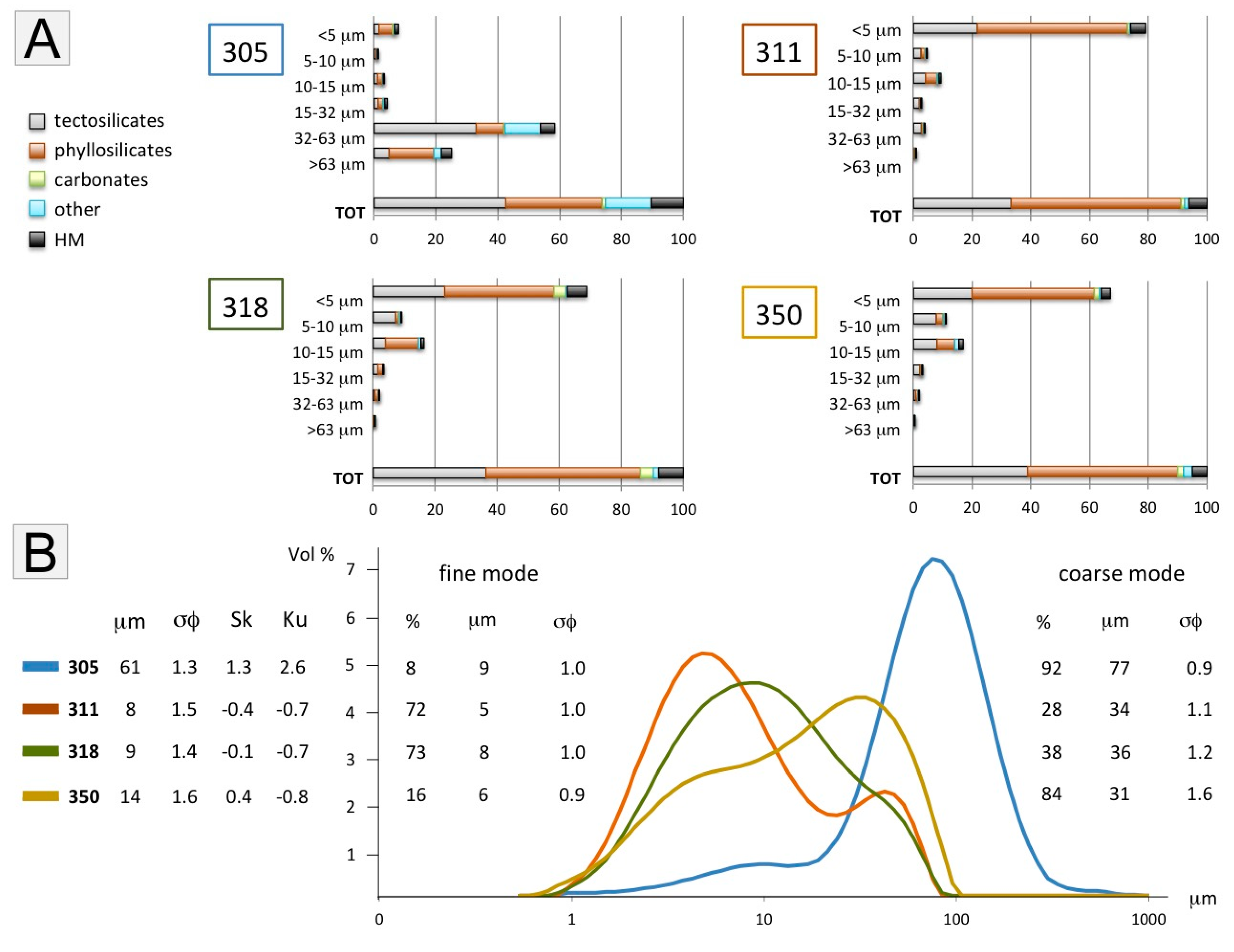
Figure 4.
Foraminifera in Bengal shelf sediments (>63 μm class for all samples). (A) Bolivinoidea superfamily, Glaessner 1937 (sample 318); (B) Planorbulinoidea superfamily, Schwager 1877 (sample 350); (C) Vaginulinidae family, Reuss 1860 (sample 318); (D) Globigerinidae family, Parker and Jones 1862 (sample 350). Scale bar for all optical images = 30 μm.

Figure 5.
Triangular diagrams illustrating the mineralogical composition of the four studied samples, and of the six size-windows analyzed for each sample by combining grain counting under the microscope and Raman spectroscopy for classes >5 μm and XRD data for the <5-μm class. (A) Qz = quartz; F = total feldspars; HM = total heavy minerals; (B) KF + NaPl = alkali feldspars (including K-feldspar, albite, and ternary feldspars); CaPl = calcium-bearing plagioclase; (C) tHM = transparent heavy minerals; (D) relative abundance of the three most common groups of transparent heavy minerals in orogenic sediments. The average composition of Ganga (g = silt; G = sand) and Brahmaputra (b = silt; B = sand) sediments (from Garzanti et al. [24]), as well as mineralogical data on Bengal Fan sediments from Thompson [13] and Yokoyama et al. [15], are given for comparison.
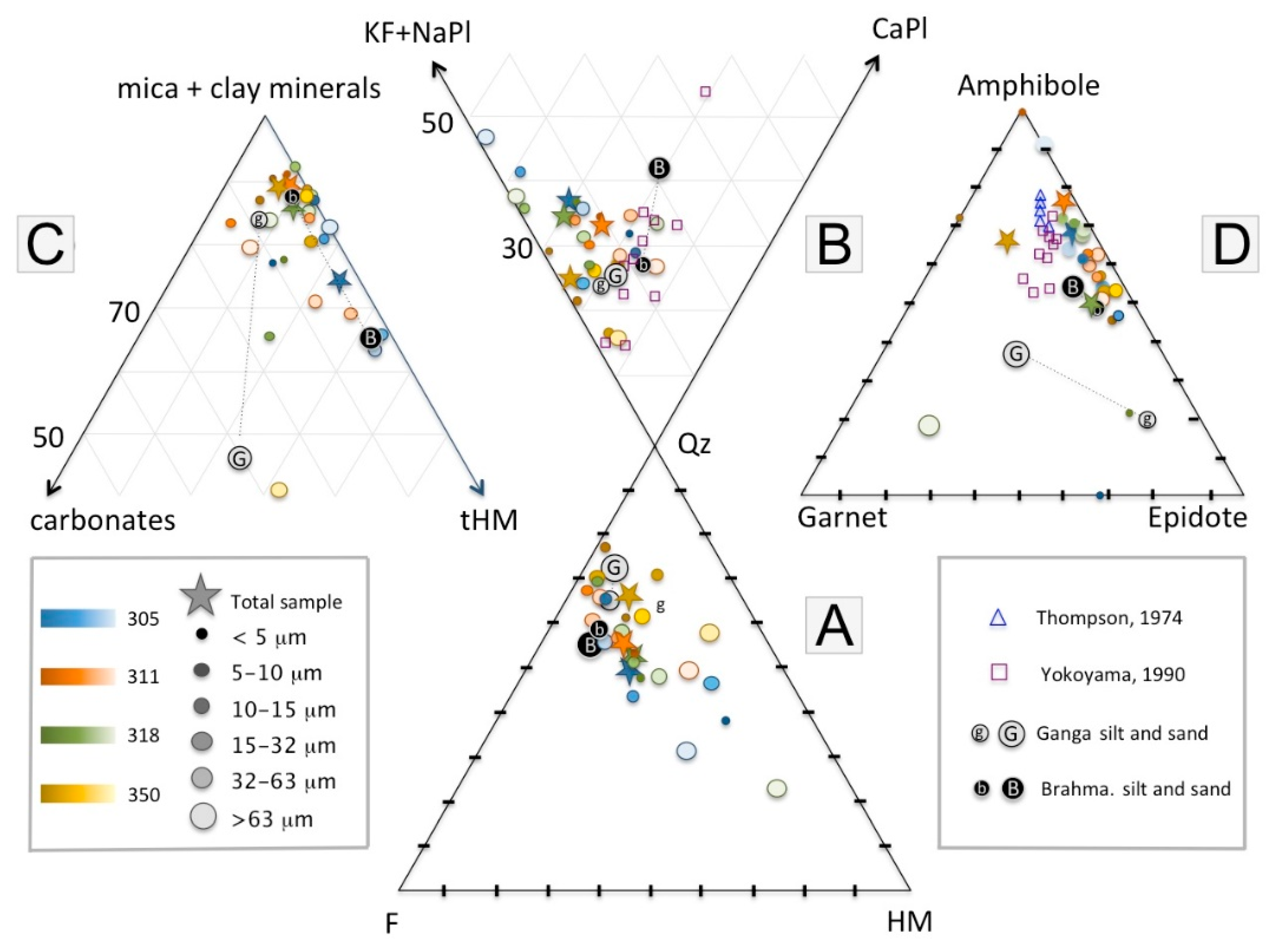
Figure 6.
Intra-sample compositional variability. In most samples, mica (muscovite + biotite + chlorite) is concentrated in the coarse tail of the grain-size distribution (GSZ, determined by wet sieving). Heavy minerals (HM) show a minimum in the tectosilicate-rich 5–10-μm class and tend to increase in coarser classes. The lack of systematic grain-size control is ascribed to bimodal grain-size distribution as a result of mixing of fine and coarse modes in different proportions.
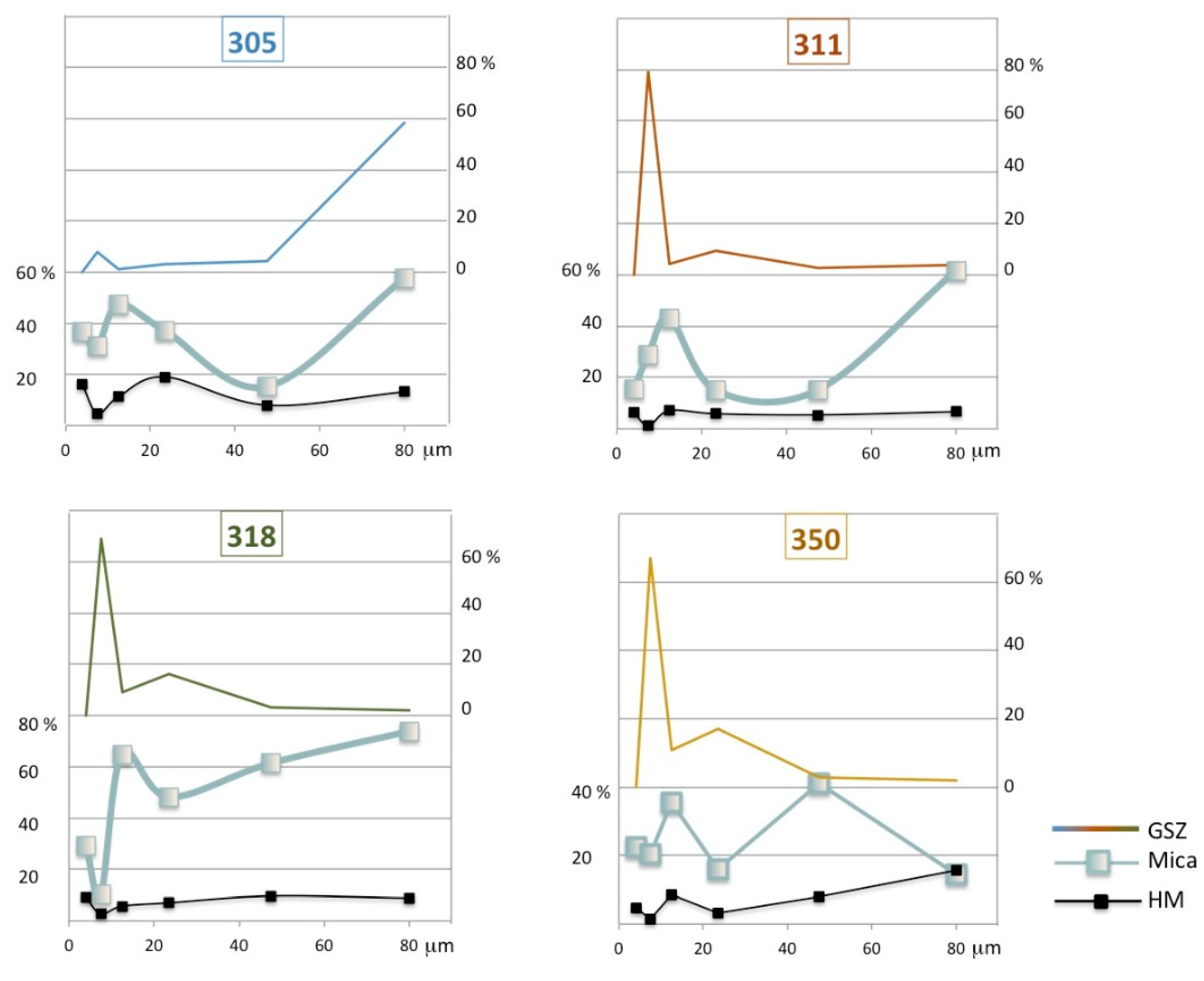
Figure 7.
Inter-sample and intra-sample variability in transparent-heavy-mineral suites. The biplot [103] drawn using CoDaPack software by Comas-Cufí and Thió-Henestrosa [104]) displays multivariate observations (points) and variables (rays). The length of each ray is proportional to the variance of each element in the dataset. If the angle between two rays is close to 0°, 90°, and 180°, then the corresponding compositional parameters are directly correlated, uncorrelated, and inversely correlated, respectively. Ap = apatite; Cld = chloritoid; Ep = epidote; Grt = garnet; Ky+Sil = kyanite + sillimanite; St = staurolite; Ttn = titanite; ZTR = zircon + tourmaline + rutile.
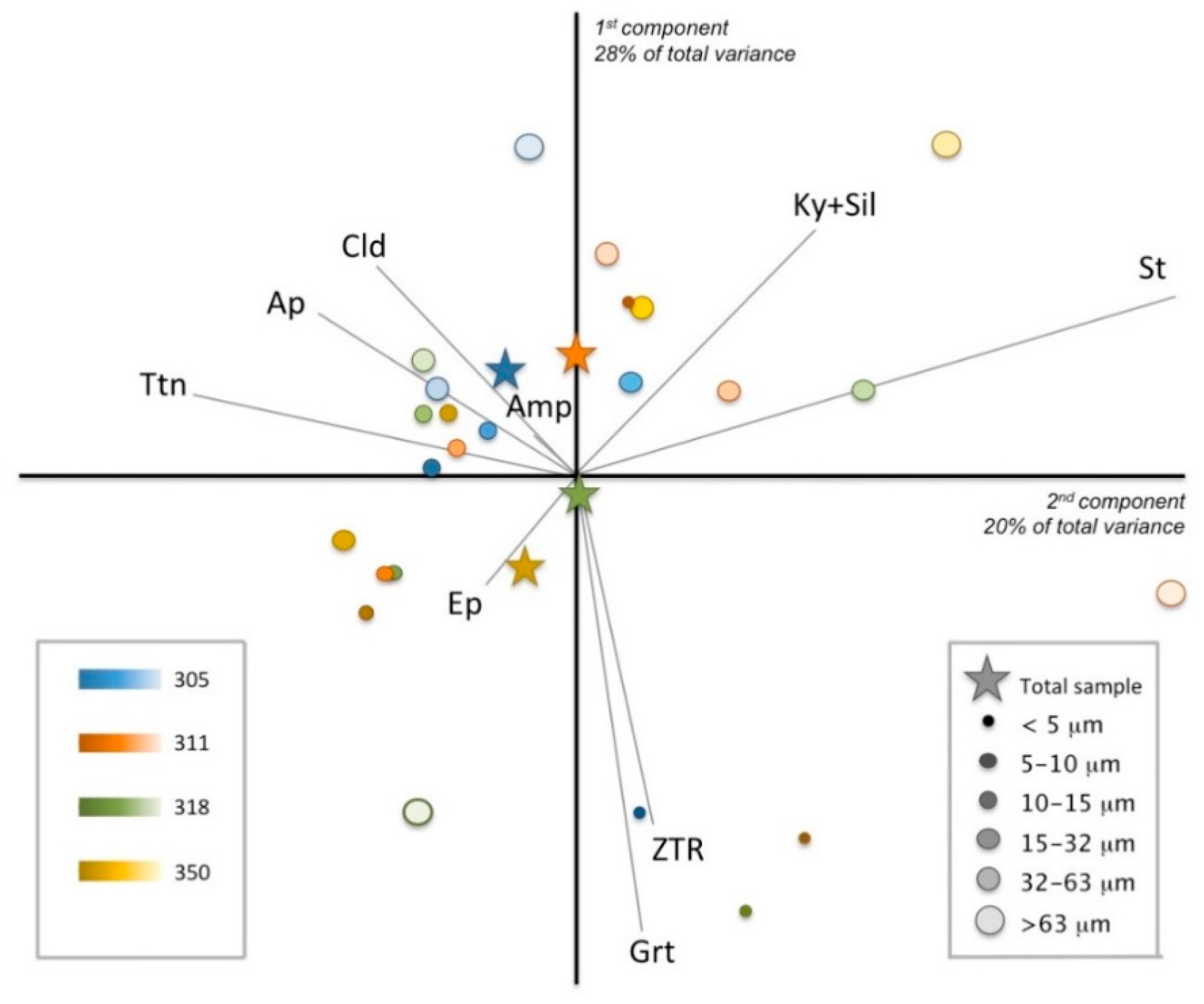
Figure 8.
Triangular diagrams illustrating the bulk-sediment geochemistry of the four studied samples. The average composition of Ganga (g = silt; G = sand) and Brahmaputra (b = silt; B = sand) sediments is given for comparison. Relatively to the very-coarse-silt sample 305, fine-silt samples 311, 318, and 350 are notably enriched in Al and K, preferentially hosted in phyllosilicates.

Figure 9.
Images of the used nylon sieves (5-μm, 10-μm, and 15-μm mesh size) with the corresponding size classes obtained for sample 318, divided into low-density (<2.90 g/cm3, “light” LM) and high-density (>2.90 g/cm3 “heavy” HM) mineral fractions. Although the sieve meshes were slightly deformed and several grains got caught into them, after this laborious procedure, we managed to obtain neatly separated grain-size classes for mineralogical analysis of cohesive mud. Red square is included for scale.

Figure 10.
Detrital modes of Bengal shelf silt compared with Ganga and Brahmaputra suspended load (size of symbols proportional to sample grain size; depth of sampling within the river channel in meters indicated close to each symbol; data after Garzanti et al. [24]. Bengal shelf sediments display Brahmaputra signature, although the most distal and finest grained sample is more akin to the Ganga. (A) Ganga silt is distinguished by higher quartz/feldspar (Q/F) and lower plagioclase/feldspar (P/F) ratios than Brahmaputra silt (arrow indicates proximal/distal trend; QPK plot after Dickinson [111]). (B) The biplot [103] based on heavy-mineral data highlights the close affinity between heavy-mineral suites in Bengal Shelf silt and suspended load in the Brahmaputra River and Meghna estuary. (C) The biplot based on the entire mineralogical dataset (both LM and HM fractions) best highlights the different signatures of Ganga and Brahmaputra suspended load (first principal component, PC1) and the grain-size effect (PC2). Because of the presence of allochemical carbonate in shelf sediments, calcite grains were not included in the biplot.
Figure 11.
Geochemistry of Ganga, Brahmaputra, Padma, and Meghna suspended load entrained at shallow (≤2 m) and greater (>5 m) channel depth compared with Bengal shelf silt (elements arranged following the periodic table group by group; data normalized to the mean composition of fine silt samples 311, 318, and 350; Table S4, Supplementary Materials). (A) The composition of fine Bengal shelf silt compares broadly with shallow suspended load in the Padma River and Meghna estuary (gray field), in turn chiefly derived from the Ganga and Brahmaputra, but with notably less Ca, Ba, U, Zr, Sn, P, and Sb. Note that the composition of very coarse Bengal shelf silt (sample 305) is a quasi-perfect mirror image of that of Ganga clay (<2 μm; own data), which allows us to see fine Bengal shelf silt as a mixture of these two end members in subequal proportions. (B) The composition of very coarse Bengal shelf silt compares rather well with deep suspended load in the Padma River and Meghna estuary (gray field), even though with lower concentration of elements preferentially hosted in ultradense minerals (REE, Zr, Hf).

Table 1.
Multiple-window bulk-sediment mineralogical data for the four studied samples obtained by combining grain counting under the microscope with Raman spectroscopy for classes >5-μm and by X-ray diffraction (XRD) for the <5-μm class (in italics). Bulk-sample composition is in bold. GSZ = Grain size (in μm); Qz = quartz; KF= K-feldspar + ternary feldspar; Ab = albite; Ca-Pl = Ca-plagioclase; Rf = rock fragments; tHM = transparent heavy minerals; Op = opaque heavy minerals; Ms = muscovite; Bt = biotite; Chl = chlorite; Cc = calcite + aragonite; Do = dolomite; Alt = altered grains; OM = Organic Matter; & = others undetermined.
| Sample | GSZ (μm) | Class (wt.%) | Qz | KF | Ab | Ca-Pl | Rf | tHM | Op | Ms | Bt | Chl | Clay | Cc | Do | Alt | OM | & | |
|---|---|---|---|---|---|---|---|---|---|---|---|---|---|---|---|---|---|---|---|
| 305 | <5 | 7.9 | 14 | 1 | 5 | 0 | 9 | 7 | 20 | 0 | 16 | 18 | 7 | 0 | 0 | 0 | 1 | 100.0 | |
| 5–10 | 1.1 | 40 | 4 | 6 | 7 | 0 | 5 | 0 | 15 | 11 | 6 | 0 | 0 | 0 | 6 | 2 | 0 | 100.0 | |
| 10–15 | 3.3 | 20 | 6 | 8 | 1 | 5 | 10 | 1 | 25 | 4 | 19 | 0 | 0 | 1 | 1 | 0 | 0 | 100.0 | |
| 15–32 | 4.3 | 23 | 2 | 5 | 1 | 12 | 19 | 0 | 19 | 0 | 18 | 0 | 0 | 1 | 0 | 0 | 0 | 100.0 | |
| 32–63 | 58.4 | 36 | 9 | 7 | 4 | 20 | 8 | 0 | 7 | 5 | 3 | 0 | 1 | 0 | 0 | 0 | 0 | 100.0 | |
| >63 | 25.0 | 10 | 4 | 5 | 0 | 7 | 12 | 1 | 31 | 10 | 17 | 0 | 0 | 0 | 3 | 0 | 0 | 100.0 | |
| Total sample | 27 | 7 | 6 | 2.9 | 14 | 10 | 0.8 | 15 | 6 | 9 | 1 | 1 | 0.1 | 0.8 | 0.0 | 0.1 | 100.0 | ||
| 311 | <5 | 79.1 | 18 | 2 | 8 | 0 | 6 | 1 | 6 | 0 | 10 | 49 | 1 | 0 | 0 | 0 | 0 | 100.0 | |
| 5–10 | 4.4 | 41 | 5 | 9 | 4 | 0 | 1 | 0 | 19 | 4 | 5 | 0 | 4 | 0 | 4 | 3 | 0 | 100.0 | |
| 10–15 | 9.4 | 29 | 5 | 7 | 3 | 3 | 7 | 0 | 35 | 2 | 6 | 0 | 0 | 1 | 3 | 0 | 0 | 100.0 | |
| 15–32 | 2.6 | 50 | 6 | 10 | 11 | 0 | 6 | 0 | 11 | 1 | 3 | 0 | 0 | 1 | 2 | 0 | 0 | 100.0 | |
| 32–63 | 3.8 | 51 | 10 | 3 | 7 | 0 | 5 | 1 | 9 | 3 | 3 | 0 | 2 | 0 | 2 | 5 | 0 | 100.0 | |
| >63 | 0.7 | 10 | 1 | 1 | 2 | 1 | 7 | 0 | 24 | 16 | 21 | 0 | 9 | 0 | 2 | 6 | 0 | 100.0 | |
| Total sample | 22 | 3 | 6 | 3.0 | 0 | 5 | 0.7 | 10 | 1 | 9 | 39 | 1 | 0.2 | 0.5 | 0.4 | 0.3 | 100.0 | ||
| 318 | <5 | 68.8 | 21 | 2 | 10 | 0 | 9 | 0 | 19 | 0 | 11 | 22 | 1 | 5 | 0 | 0 | 1 | 100.0 | |
| 5–10 | 9.2 | 58 | 3 | 14 | 3 | 0 | 3 | 0 | 9 | 0 | 1 | 0 | 0 | 3 | 3 | 3 | 0 | 100.0 | |
| 10–15 | 16.4 | 16 | 6 | 3 | 0 | 1 | 6 | 0 | 35 | 7 | 23 | 0 | 0 | 0 | 3 | 1 | 0 | 100.0 | |
| 15–32 | 3.4 | 31 | 3 | 9 | 3 | 0 | 7 | 0 | 21 | 19 | 8 | 0 | 0 | 0 | 0 | 0 | 0 | 100.0 | |
| 32–63 | 1.9 | 18 | 5 | 0 | 5 | 0 | 10 | 0 | 33 | 24 | 5 | 0 | 1 | 0 | 1 | 0 | 0 | 100.0 | |
| >63 | 0.4 | 3 | 1 | 1 | 0 | 1 | 8 | 1 | 21 | 48 | 4 | 0 | 7 | 0 | 2 | 1 | 0 | 100.0 | |
| Total sample | 21 | 4 | 5 | 1.5 | 0 | 8 | 0.0 | 26 | 6 | 15 | 8 | 0 | 2.0 | 1.7 | 0.5 | 0.3 | 100.4 | ||
| 350 | <5 | 67.1 | 21 | 2 | 6 | 0 | 4 | 1 | 13 | 0 | 10 | 40 | 2 | 1 | 0 | 0 | 1 | 100.0 | |
| 5–10 | 11.0 | 56 | 3 | 13 | 0 | 0 | 1 | 0 | 12 | 2 | 7 | 0 | 2 | 0 | 1 | 4 | 0 | 100.0 | |
| 10–15 | 16.9 | 40 | 1 | 6 | 1 | 7 | 5 | 3 | 28 | 0 | 7 | 0 | 0 | 0 | 2 | 0 | 0 | 100.0 | |
| 15–32 | 2.9 | 56 | 5 | 10 | 6 | 1 | 3 | 0 | 8 | 6 | 1 | 0 | 0 | 1 | 2 | 0 | 0 | 100.0 | |
| 32–63 | 1.9 | 29 | 4 | 5 | 2 | 7 | 6 | 2 | 21 | 11 | 8 | 0 | 0 | 0 | 5 | 0 | 0 | 100.0 | |
| >63 | 0.2 | 29 | 4 | 1 | 1 | 12 | 11 | 5 | 5 | 2 | 7 | 0 | 10 | 0 | 1 | 13 | 0 | 100.0 | |
| Total sample | 29 | 2 | 7 | 0.4 | 1 | 4 | 1.0 | 15 | 1 | 9 | 27 | 1 | 0.6 | 0.5 | 0.5 | 0.6 | 100.0 | ||
Table 2.
Multiple-window heavy-mineral data for the four studied samples obtained by combining grain counting under the microscope with Raman spectroscopy for classes >5 μm and by XRD for the <5 μm class. Bulk-sample composition is in bold; XRD data, in italics, are only indicative and were not considered in the calculation of bulk-sample composition; GSZ = Grain size (in μm); tHMC = transparent-heavy-mineral concentration; Zrn = zircon; Tur = tourmaline; Rt = rutile; TiOx = anatase + brookite; Ttn = titanite; Ap = apatite; Ep = epidote; Grt = garnet; Cld = chloritoid; St = staurolite; Ky = kyanite; Sil = sillimanite; Amp = amphibole; Px = pyroxene; &tHM = orthopyroxene, baryte, Cr-spinel, monazite, olivine, or xenotime. The weight percentage of each class was obtained by wet sieving; n.d. = not determined; tr. = in trace.
| Sample | GSZ (μm) | Class (%) | tHMC | Zrn | Tur | Rt | TiOx | Ttn | Ap | Ep | Grt | Cld | St | Ky + Sil | Amp | Px | &tHM | |
|---|---|---|---|---|---|---|---|---|---|---|---|---|---|---|---|---|---|---|
| 305 | <5 | 7.9 | 9 | 2 | 0 | 0 | 0 | 3 | 43 | 20 | 0 | 0 | 0 | 30 | 2 | 100 | ||
| 5–10 | 1.1 | 5 | 1 | 1 | 2 | 3 | 3 | 2 | 28 | 4 | 1 | 0 | 0.4 | 50 | 4 | 0 | 100 | |
| 10–15 | 3.3 | 10 | 1 | 5 | 2 | 1 | 3 | 1 | 38 | 4 | 2 | 0 | 4 | 37 | 2 | 2 | 100 | |
| 15–32 | 4.3 | 19 | 1 | 5 | 3 | 0 | 5 | 1 | 31 | 4 | 2 | 1 | 1 | 41 | 4 | 0 | 100 | |
| 32–63 | 58.4 | 8 | 0 | 2 | 1 | 1 | 5 | 2 | 25 | 5 | 2 | 0 | 2 | 52 | 4 | 0 | 100 | |
| >63 | 25.0 | 12 | 0 | 0 | 0 | 0 | 0 | 7 | 7 | 0 | 0 | 0 | 0 | 73 | 13 | 0 | 100 | |
| Total sample | 10 | 0.1 | 2 | 0.7 | 0.3 | 3 | 4 | 20 | 3 | 1 | 0 | 1 | 58 | 7 | 0.1 | 100 | ||
| 311 | <5 | 79.1 | 6 | 4 | 0 | 0 | 0 | 6 | 0 | 0 | 0 | 0 | 0 | 90 | 0 | 100 | ||
| 5–10 | 4.4 | 1 | 0 | 1 | 2 | 1 | 2 | 1 | 30 | 4 | 1 | 0 | 0 | 56 | 2 | 0 | 100 | |
| 10–15 | 9.4 | 7 | 1 | 2 | 2 | 1 | 5 | 1 | 32 | 4 | 1 | 0 | 2 | 47 | 2 | 1 | 100 | |
| 15–32 | 2.6 | 6 | 0 | 2 | 0 | 0 | 4 | 0 | 28 | 5 | 4 | 1 | 2 | 49 | 7 | 0 | 100 | |
| 32–63 | 3.8 | 5 | 1 | 1 | 1 | 0 | 3 | 3 | 28 | 2 | 3 | 1 | 1 | 51 | 7 | 0 | 100 | |
| >63 | 0.7 | 7 | 4 | 6 | 4 | 0 | 0 | 0 | 33 | 6 | 0 | 6 | 4 | 39 | 0 | 0 | 100 | |
| Total sample | 5 | 0.9 | 2 | 1 | 0.4 | 4 | 1 | 31 | 4 | 2 | 0.4 | 1 | 48 | 3 | 1 | 100 | ||
| 318 | <5 | 68.8 | 9 | 0 | 0 | 13 | 0 | 0 | 41 | 9 | 0 | 0 | 0 | 37 | 0 | 100 | ||
| 5–10 | 9.2 | 3 | 1 | 2 | 1 | 0 | 3 | 1 | 21 | 3 | 1 | 0 | 0 | 62 | 4 | 0 | 100 | |
| 10–15 | 16.4 | 6 | 1 | 2 | 2 | 1 | 5 | 3 | 20 | 5 | 2 | 0 | 1 | 61 | 0 | 1 | 100 | |
| 15–32 | 3.4 | 7 | 1 | 1 | 0 | 0 | 0 | 1 | 27 | 3 | 1 | 1 | 1 | 62 | 4 | 0 | 100 | |
| 32–63 | 1.9 | 10 | 1 | 1 | 0 | 0 | 3 | 2 | 24 | 2 | 3 | 0 | 1 | 57 | 7 | 1 | 100 | |
| >63 | 0.4 | 8 | 7 | 7 | 0 | 0 | 10 | 3 | 13 | 43 | 0 | 0 | 0 | 13 | 3 | 0 | 100 | |
| Total sample | 8 | 0.7 | 2 | 1 | 0.3 | 4 | 2 | 21 | 4 | 1 | 0.1 | 1 | 60 | 2 | 1 | 100 | ||
| 350 | <5 | 67.1 | 4 | 0 | 0 | 14 | 0 | 0 | 0 | 23 | 0 | 0 | 0 | 55 | 8 | 100 | ||
| 5–10 | 11.0 | 1 | 4 | 6 | 3 | 1 | 3 | 1 | 34 | 5 | 2 | 0 | 0 | 33 | 6 | 1 | 100 | |
| 10–15 | 16.9 | 5 | 2 | 4 | 2 | 3 | 3 | 2 | 29 | 4 | 4 | 0 | 2 | 45 | 1 | 1 | 100 | |
| 15–32 | 2.9 | 3 | 1 | 3 | 3 | 0 | 3 | 2 | 34 | 4 | 7 | 0 | 0 | 45 | 1 | 0 | 100 | |
| 32–63 | 1.9 | 6 | 0 | 2 | 1 | 0 | 5 | 1 | 37 | 3 | 4 | 1 | 2 | 46 | 2 | 0 | 100 | |
| >63 | 0.2 | 11 | n.d. | n.d. | n.d. | n.d. | n.d. | n.d. | n.d. | n.d. | n.d. | tr. | n.d. | n.d. | n.d. | n.d. | ||
| Total sample | 4 | 2 | 4 | 2 | 2 | 3 | 2 | 31 | 4 | 4 | 0 | 2 | 44 | 1 | 1 | 100 | ||
© 2019 by the authors. Licensee MDPI, Basel, Switzerland. This article is an open access article distributed under the terms and conditions of the Creative Commons Attribution (CC BY) license (http://creativecommons.org/licenses/by/4.0/).
Share and Cite
MDPI and ACS Style
Borromeo, L.; Andò, S.; France-Lanord, C.; Coletti, G.; Hahn, A.; Garzanti, E. Provenance of Bengal Shelf Sediments: 1. Mineralogy and Geochemistry of Silt. Minerals 2019, 9, 640. https://doi.org/10.3390/min9100640
AMA Style
Borromeo L, Andò S, France-Lanord C, Coletti G, Hahn A, Garzanti E. Provenance of Bengal Shelf Sediments: 1. Mineralogy and Geochemistry of Silt. Minerals. 2019; 9(10):640. https://doi.org/10.3390/min9100640
Chicago/Turabian StyleBorromeo, Laura, Sergio Andò, Christian France-Lanord, Giovanni Coletti, Annette Hahn, and Eduardo Garzanti. 2019. "Provenance of Bengal Shelf Sediments: 1. Mineralogy and Geochemistry of Silt" Minerals 9, no. 10: 640. https://doi.org/10.3390/min9100640
Note that from the first issue of 2016, this journal uses article numbers instead of page numbers. See further details here.