Viscoelastic Behaviour from Complementary Forced-Oscillation and Microcreep Tests

Abstract

There is an important complementarity between experimental methods for the study of high-temperature viscoelasticity in the time and frequency domains that has not always been fully exploited. Here, we show that the parallel processing of forced-oscillation data and microcreep records, involving the consistent use of either Andrade or extended Burgers creep function models, yields a robust composite modulus-dissipation dataset spanning a broader range of periods than either technique alone. In fitting this dataset, the alternative Andrade and extended Burgers models differ in their partitioning of strain between the anelastic and viscous contributions. The extended Burgers model is preferred because it involves a finite range of anelastic relaxation times and, accordingly, a well-defined anelastic relaxation strength. The new strategy offers the prospect of better constraining the transition between transient and steady-state creep or, equivalently, between anelastic and viscous behaviour.

1. Introduction

Viscoelastic relaxation at small strain amplitudes is of geophysical significance as the cause of the attenuation and frequency-dependent wavespeeds (dispersion) of seismic waves within the Earth’s deep interior [1,2,3]. For example, Minster and Anderson [4] demonstrated the potentially important link between dislocation creep and seismic-wave attenuation, and Karato [5] showed how the temperature sensitivity of wavespeeds is enhanced by viscoelastic relaxation.

In a very influential contribution, Goetze [6] reviewed the extensive literature concerning internal friction in metals, measured mainly with resonance (torsional pendulum) techniques, and emphasized the need for high-temperature laboratory measurements on geological materials at sub-Hz teleseismic frequencies rather than the MHz frequencies of conventional laboratory wave-propagation methods. This challenge has been addressed mainly with superior sub-resonant forced-oscillation techniques in multiple laboratories worldwide (e.g., [7,8,9,10,11,12]).

Concerning such methods for the study of high-temperature viscoelasticity, it is well known that there is, in principle, a valuable complementarity between time-domain and frequency- (or period-) domain methods (e.g., [13]). In practice, time-domain microcreep studies have been used to constrain the value of steady-state viscosity for use in modelling the results of sub-resonant forced oscillation studies [10,11]. In our laboratory, consistency between forced-oscillation and microcreep data has been used as evidence of linearity of mechanical behaviour [14], and microcreep studies have been used to provide a qualitative or quantitative indication of the extent to which the inelastic strain is recoverable on removal of the applied stress [15,16]. However, we have not yet fully exploited the valuable complementarity between the forced-oscillation and microcreep methods. The purpose of this investigation is to explore how results obtained in our laboratory from the two methods might best be combined to take advantage of the complementarity.

If a steady stress is suddenly applied at time t = 0, i.e., σ(t) = H(t), where H is the Heaviside step function, the resulting strain is specified by the creep function J(t). Provided only that the mechanical behaviour is linear, the strain ε(t) = ε₀exp(iωt − δ) associated with a stress σ(t) = σ₀exp(iωt), that is sinusoidally time-varying with angular frequency ω, may be calculated by superposition of the strains resulting from a series of consecutive step-function changes in stress each of infinitesimal amplitude. In this way, it is established that

ε(t) = J*(ω)σ(t)

(1)

where the (complex) dynamic compliance J*(ω) is related to the creep function J(t) by (e.g., [13,17]).

$$J^{*}(\omega )=i\omega {\displaystyle \underset{0}{\overset{\infty }{\int }}J(\xi )\exp (-i\omega \xi )d\xi }$$

(2)

In the representation of linear viscoelastic behaviour, the alternative Andrade and extended Burgers creep functions J(t), respectively,

J(t) = J_U + βtⁿ + t/η

(3)

and

$$J(t)=J_U\{1+\Delta {\displaystyle \underset{-\infty }{\overset{\infty }{\int }}D(\ln \tau )[1-\exp (-t/\tau )]d\ln \tau \}+t/\eta }$$

(4)

are widely used. In Equations (3) and (4), J_U is the unrelaxed compliance, β is the coefficient of the term representing the transient creep varying as the fractional n-th power of time t, and η is the steady-state viscosity. For the Burgers model, the parameter Δ is the anelastic relaxation strength associated with the distribution D(lnτ) of anelastic relaxation times.

The distribution D(lnτ) of anelastic relaxation times is commonly prescribed by separately normalised contributions D_B(lnτ) and D_P(lnτ), appropriate for monotonic dissipation background and a superimposed peak, respectively, along with the associated modulus dispersion:

D_B(lnτ) = ατ^α/(τ_H^α − τ_L^α), for τ_L ≤ τ ≤ τ_H, and zero elsewhere [4,18].

D_P(lnτ) = σ⁻¹(2π)^−1/2exp{−[ln(τ/τ_P)/σ]²}.

(5)

In Equation (5), τ_L and τ_H are respectively the lower and upper limits of the distribution of anelastic relaxation times τ, and α the τ-exponent in the distribution D_B(lnτ). The parameters τ_P and σ define the centre and width, respectively, of the log-normal distribution of relaxation times given by D_P(lnτ). The duration of transient creep involving grain-boundary sliding has been identified with the Maxwell time τ_M = ηJ_U [19]. Accordingly, consistent with insights from more recent micromechanical modelling of grain-boundary sliding [20] and our recent practice [16], we here set τ_H = τ_M.

The real and negative imaginary parts of the associated dynamic compliance J*(ω) = J₁(ω) − iJ₂(ω) for the Andrade model are

J₁(ω) = J_U + βΓ(1 + n)ω⁻ⁿcos(nπ/2)
J₂(ω) = βΓ(1 + n)ω⁻ⁿsin(nπ/2) + 1/ηω.

(6)

The corresponding quantities for the extended Burgers model are

$$\begin{gathered} J_1(\omega )=J_U\{1+\Delta {\displaystyle \underset{-\infty }{\overset{\infty }{\int }}D(\ln \tau )d\ln \tau /(1+{\omega }^2{\tau }^2)\}} \\ {J}_2(\omega )=\omega J_U\Delta {\displaystyle \underset{-\infty }{\overset{\infty }{\int }}\tau D(\ln \tau )d\ln \tau /(1+{\omega }^2{\tau }^2)}+1/\eta \omega . \end{gathered}$$

(7)

In equivalent parameterisations, the Maxwell time τ_M = ηJ_U takes the place of viscosity η.

The (stiffness) modulus M(ω) and strain energy dissipation Q⁻¹(ω) then follow as

M(ω) = [J₁²(ω) + J₂²(ω)]^−1/2 and Q⁻¹(ω) = J₂(ω)/J₁(ω).

(8)

Accordingly, it is seen that, in principle, the creep function J(t) and the dynamic compliance J*(ω) contain identical information concerning the mechanical behaviour.

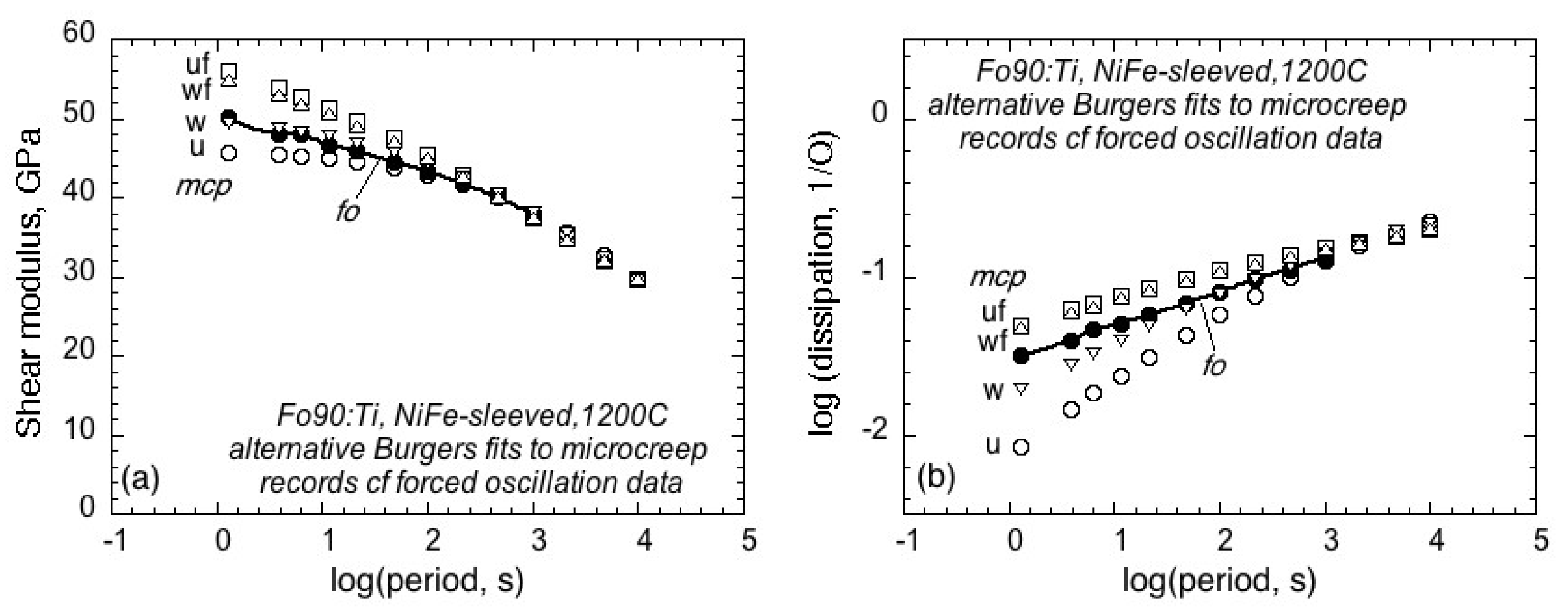
In practice, however, there are two important qualifications. Forced-oscillation measurements of shear modulus G (or Young’s modulus E) and associated strain-energy dissipation Q⁻¹ involve comparison of stress and strain signals of prescribed frequency or period (T_o) that are intensively sampled—even at short periods. In contrast, microcreep records, of much longer duration, are normally much more sparsely sampled. Thus, in our laboratory, the forced-oscillation and microcreep records are routinely sampled at frequencies of 128/T_o and 1 Hz, respectively. Accordingly, forced-oscillation data are expected to better resolve the behaviour at short timescales, whereas microcreep records will better resolve the behaviour at long timescales. Furthermore, our microcreep testing protocol involving successive switching of the torque between steady values 0, +L, 0, −L, and 0 has the capacity to distinguish between recoverable (and therefore anelastic) and permanent (viscous) strains, as demonstrated below. Forced-oscillation records comprising multiple complete cycles of oscillation have no such capacity to distinguish between anelastic and viscous behaviour.

2. Materials and Methods

2.1. The Processing of Experimental Forced-Oscillation Data

In our laboratory, shear modulus G and dissipation Q⁻¹ are measured at each prescribed oscillation period T_o by comparing the complex torsional compliances (rad (Nm)⁻¹) measured on complementary experimental assemblies containing, respectively, the cylindrical specimen of interest and a control specimen of known, nearly elastic, shear modulus [9]. Calculation of the compliance differential between the two assemblies serves to eliminate the contribution to the overall compliance from ceramic/steel torsion rods in series mechanically with the specimens. Accordingly, the compliance differential is the difference in compliance between the metal-jacketed specimen and a similarly jacketed control specimen of either polycrystalline alumina or a sapphire crystal. The compliances of the respective assemblies are routinely corrected for the small perturbation caused by interaction between the gas (argon) pressure medium and the central plate moving between the pair of relatively closely spaced outer fixed plates of the capacitance displacement transducers [21]. The force exerted by the gas medium on the central plate perturbs the observed compliance both by bending the lever arms on which the transducer central plates are mounted and by contributing to the torque. If the space between two parallel circular plates of radius R is occupied by gas (argon) of density ρ and viscosity η, the force F(t) on the plate with normal displacement d(t) = d₀exp(iωt) is

F(t) = −{πρω²R⁴/8h[(b/2)⁻¹tanh(b/2) − 1]} × d(t)

(9)

with

b = (1 + i)h/δ, and boundary layer thickness δ = (2η/ρω)^1/2.

(10)

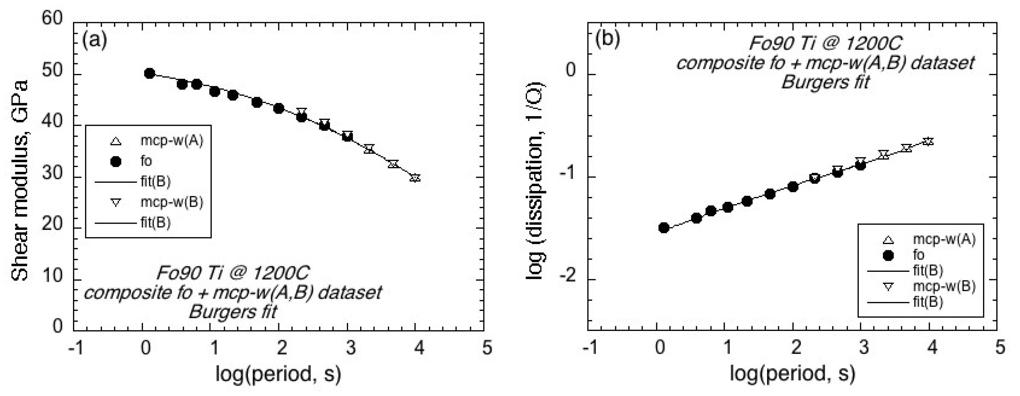
The compliance differential is also corrected for any small differences between the dimensions and jacketing of the two specimens. Established procedures for the routine processing of such forced-oscillation data for each of a series of oscillation periods T_o, approximately logarithmically equally spaced at each temperature T, are outlined in previous publications [9,22]. All such G and Q⁻¹ data obtained at relatively high temperatures and oscillation periods of 1–1000 s with logQ⁻¹ > −2.2 are then usually fitted by a non-linear least-squares procedure to an extended Burgers creep function model (e.g., [23]).

2.2. The Processing of Complementary Torsional Microcreep Records

Torsional microcreep tests in our laboratory, conducted on the same assembly as for the forced-oscillation measurements, involve the application of a torque of amplitude 0, +L, 0, −L, and 0 for successive time intervals typically of 2000 s duration each [4]. The first segment is used to estimate and correct for any linear drift, leaving a four-segment record of 8000 s duration within which the torque is switched at times t_i, (i = 1, 2, 3, 4). The switching of the torque can be modelled as the superposition of Heaviside step functions of appropriate sign s_i (+1 at t₁ and t₄, −1 at t₂ and t₃) with rise times of order 1 s.

The motion of the central transducer plate relative to the pair of fixed plates following each such switching of the steady torque is well approximated by the expression

d(t) = d₀[1 − exp(−κt) + γt].

(11)

The force exerted by the gas medium on the moving plate is found from an analysis similar to that of [21] to be

F(t) = −3πR⁴ηγd₀/2h³ − πκ²ρR⁴d₀exp(−κt)/{8h[(b/2)⁻¹tan(b/2) − 1]}

(12)

with

b = h/δ, and boundary layer thickness now δ = (η/κρ)^1/2.

(13)

In Equation (12), the first term on the right-hand side is the force associated with the steady rate d₀γ of plate separation, whereas the second term relates to the transiently enhanced rate κd₀exp(−κt) of plate separation. Representative second-segment microcreep data have been fitted to Equation (11), allowing calculation of and correction for the influence of the forces (Equation (12)) exerted on the moving transducer plates. The resulting perturbations are of order 0.001 μm at t = 1 s—negligible when compared with displacement amplitudes of 50–100 μm. By comparison, the correction for forced-oscillation displacement amplitudes of similar magnitude at the shortest period of 1.28 s is of order 0.1 μm—large enough to justify their routine correction.

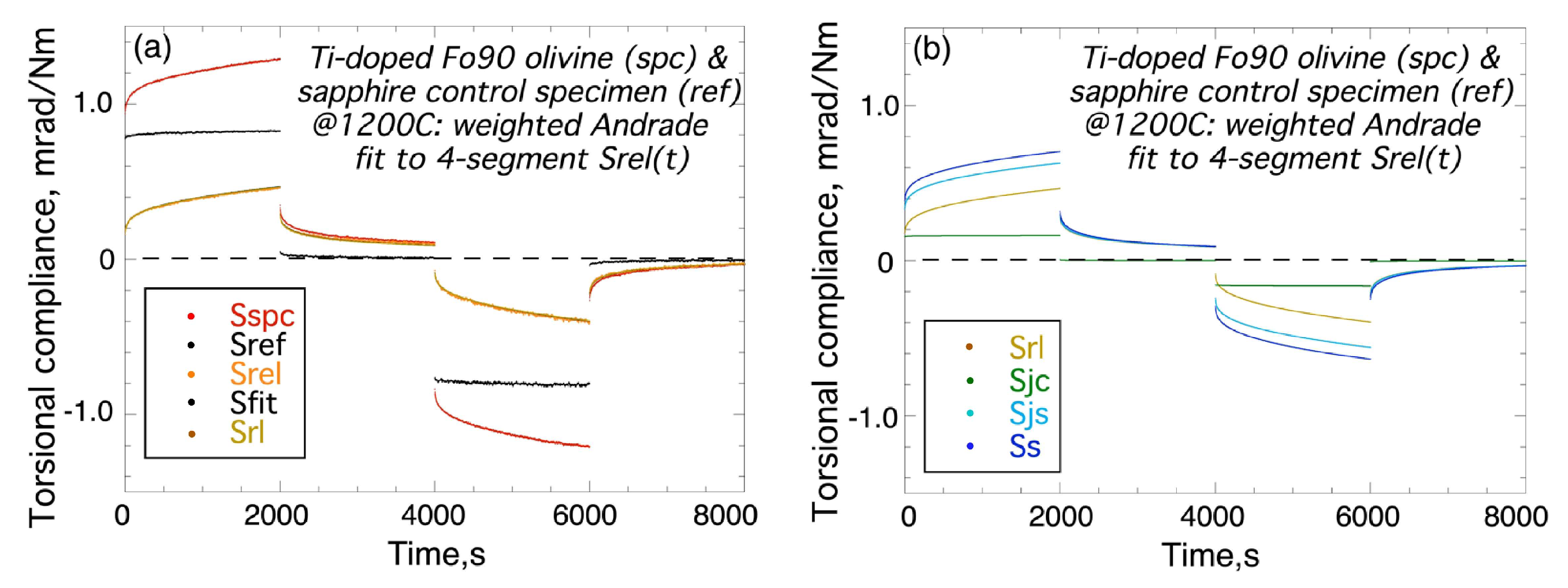
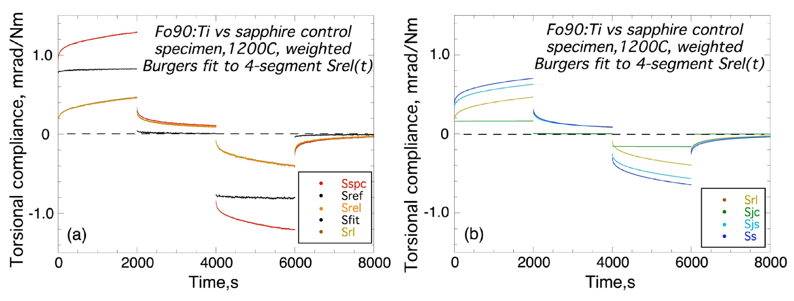
Accordingly, the raw microcreep data are first processed to obtain a quantity termed the instantaneous torsional compliance S_spc(t), being the time-dependent twist (radian) per unit torque (Nm) for the specimen assembly containing the polycrystalline specimen sandwiched between torsion rods within the enclosing metal jacket. Subtraction of the corresponding twist per unit torque for the reference assembly, S_ref(t), in which a control specimen (either Lucalox^TM polycrystalline alumina or sapphire) of known properties is substituted for the specimen, eliminates the unwanted contribution from the steel and alumina torsion rods. The difference S_rel(t) is thus the twist of the jacketed specimen relative to that of the jacketed control specimen, yet to be corrected for any (usually minor) differences in geometry. This difference signal S_rel(t) is fitted to a function S_fit(t) that is the superposition of the responses to each of the torque switching episodes, prescribed by the appropriate creep function J(t′):

S_fit(t) = Σ_i=1,ks_iJ(t_i′)

(14)

where t_i’ = t − t_i is the time elapsed since the i-th switching of the torque, for time t belonging to the k–th (k = 1, 4) segment of the four-segment record.

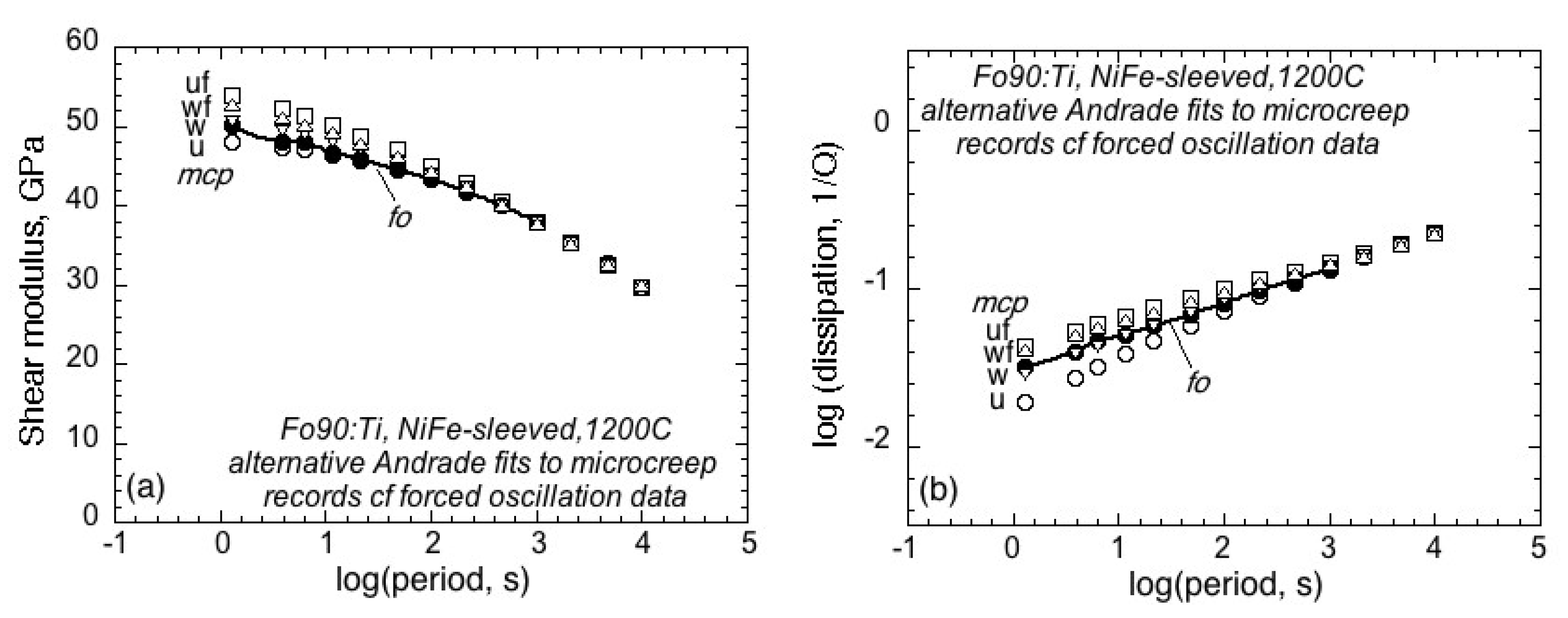
We have explored the option of weighting the fit by specifying an uncertainty in S_rel(t) proportional to logt_j′, t_j′ being the time elapsed since the most recent (k–th) switching of the torque. The effect is to weight the data early in each segment relatively more heavily—in order to strengthen the connection with the forced-oscillation data. For the same reason, it may be desirable, as explored in the Results section, to fix certain parameters in the creep function model at values constrained by the forced oscillation data. For reasons of parametric economy, the Andrade creep function (Equation (3)) has thus far been preferred over the extended Burgers alternative (Equation (4)) for use in Equation (14) [16].

The Andrade creep function J(t) associated with this time-domain fit is then Laplace transformed to obtain the corresponding complex dynamic compliance at selected periods T_o (those of the forced-oscillation experiments within the range 1–1000 s, and similarly chosen periods within the range 1000–10,000 s). The further processing of the microcreep data then proceeds exactly as for the forced-oscillation data. For the purpose of reconciling the results of the forced-oscillation and microcreep tests, the critical step in the processing of the microcreep record is therefore the fitting of the differential compliance S_rel(t) to Equation (14).

A normally very small correction is then applied to the Laplace transform of S_rel(t) for any differences in geometry between the two assemblies, to obtain the relative dynamic torsional compliance S_rl(T_o). S_rl(T_o) is added to the dynamic torsional compliance S_jc(T_o) calculated a priori for the jacketted control specimen from forced-oscillation data for the relevant jacket metal, along with data concerning the viscoelasticity of polycrystalline alumina, or appropriate temperature-dependent elastic properties of single-crystal sapphire. The result is an estimate of the dynamic torsional compliance S_js(T_o) of the jacketted specimen. The reciprocal of S_js, the torsional stiffness (Nm rad⁻¹), is then corrected for the stiffness of the jacket (inclusive of any foil wrapper used to control redox conditions), and inverted to obtain the (complex) dynamic torsional compliance S_s(T_o) of the bare cylindrical specimen from which its shear modulus G and dissipation Q⁻¹ are calculated. At each stage of this process, conducted within the period domain, the dynamic torsional compliance, fitted to an Andrade creep function, allows the construction of an associated virtual microcreep record by superposition of the responses to the successive episodes of torque switching (through Equation (14)). The results for S_rl(t), S_jc(t), S_js(t) and S_s(t) are intended to provide a clear indication of the relative contributions of the control specimen and jacket (inclusive of any liner) to the observed behaviour.

Concerning the recoverability of the strain, we first examine the use of the Andrade creep function in Equation (14) for the fit to the instantaneous torsional compliance within the second segment of the four-segment record as follows

S_fit(t) = Σ_i=1,2s_i−J(t_i′) = β[(t − t₁)ⁿ − (t − t₂)ⁿ] + (t₂ − t₁)/η.

(15)

For t >> t_i (i = 1, 2), this expression becomes approximately

S_fit(t) ≈ nβ(t₂ − t₁)t^{n − 1}+ (t₂ − t₁)/η.

(16)

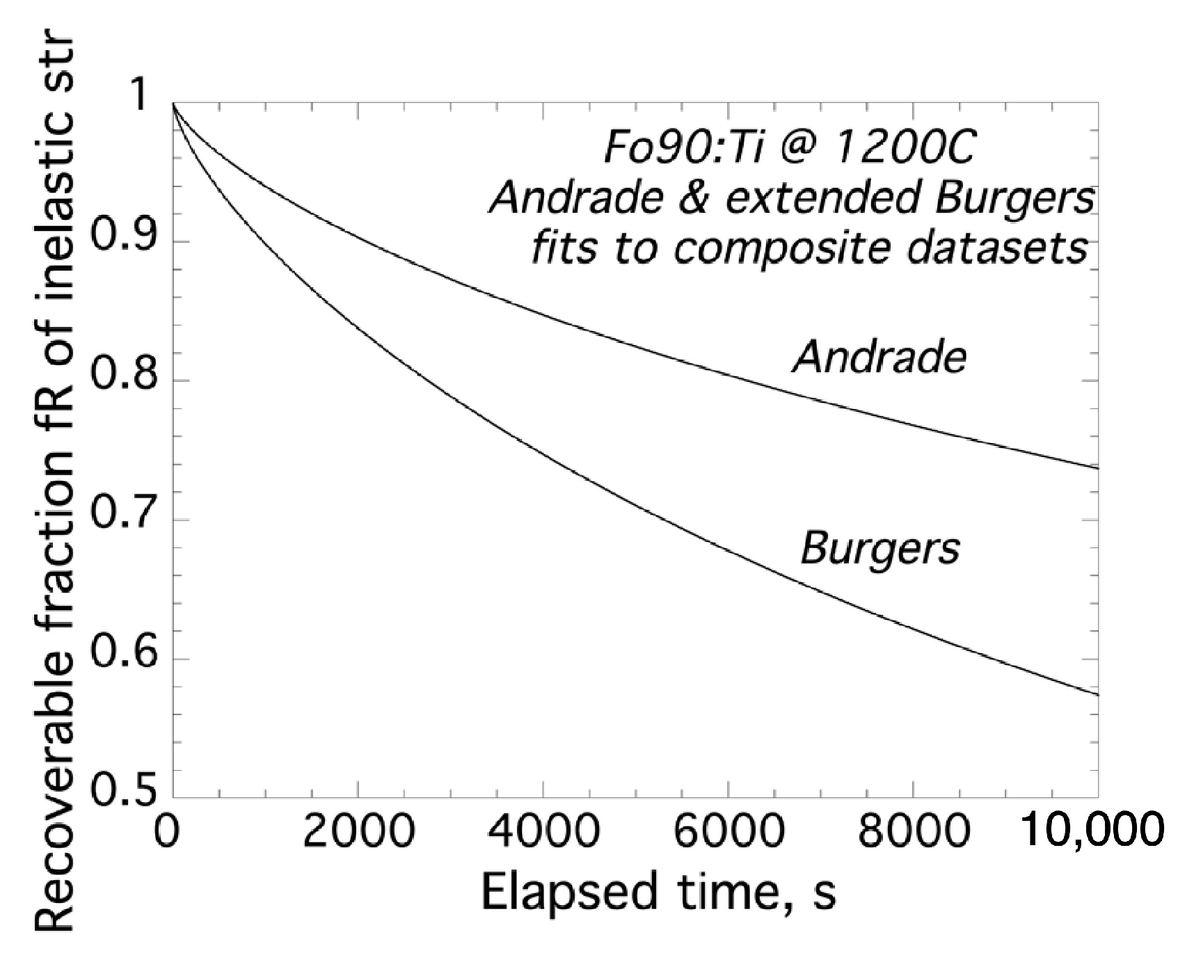
Thus, as t → ∞, the first term in Equation (16) with n typically ~1/3 becomes vanishingly small, indicating that the strain associated with the βtⁿ term in the Andrade creep function is ultimately recoverable.

Accordingly, the fraction f_R of the total inelastic strain βtⁿ + t/η at time t that is ultimately recoverable following removal of the applied torque is [16].

f_R = βtⁿ/(βtⁿ + t/η) = 1/(1 + t^{1 − n}/βη)

(17)

Such an estimate can be made for the Andrade model S_fit(t) fitted to the compliance difference S_rel(t) between the raw microcreep records right through to the Andrade model fitted to the final S_s(T_o) data—with closely consistent results concerning the fraction of recoverable strain.

For the alternative extended Burgers model, the fraction f_R of the inelastic strain that is recoverable varies with elapsed time t as

$$f_{\mathrm{R}}=\Delta {\displaystyle \underset{-\infty }{\overset{\infty }{\int }}D(\ln \tau )[1-\exp (-t/\tau })d\ln \tau /[\Delta {\displaystyle \underset{-\infty }{\overset{\infty }{\int }}D(\ln \tau )[1-\exp (-t/\tau )]d\ln \tau +t/{\tau }_M}]$$

(18)

3. Results

3.1. Reconciliation of Forced-Oscillation and Microcreep Data with the Andrade Model

Our established procedure for the processing of forced-oscillation data was applied to representative results, obtained at 1200 °C and 200 MPa, for a specimen assembly containing an Ni₇₀Fe₃₀-sleeved Ti-doped Fo₉₀ olivine specimen and for a reference assembly containing a similarly sleeved sapphire control specimen [23]. The fact that the forced-oscillation data best resolve the behaviour at relatively short periods was highlighted by the experience of fitting the Andrade model to forced-oscillation data spanning the period range 1–1000 s. It proved possible to refine the values of the parameters J_U, n, and β, but for the viscosity η, only a minimum value near 0.4 × 10⁶ GPa.s compatible with the data could be established. The resulting period-dependent values of the shear modulus G and dissipation Q⁻¹, thus derived from forced-oscillation data, will later be compared with the same quantities inferred from the microcreep records.

The previously described procedure for the processing of microcreep data [16] was applied to the complementary microcreep record (Figure 1) for the same specimen and reference assemblies under the same conditions (1200 °C and 200 MPa). The viscoelastic behaviour, calculated a priori, for the jacketed sapphire control specimen (‘jc’ in Figure 1b) and the behaviour of the reference assembly as a whole (‘ref’ in Figure 1a) reveal a close approach to perfectly elastic behaviour. Small departures from the elastic ideal are attributable to the high-temperature viscoelasticity of the metallic materials of jacket and liner, and of the ceramic torsion rods.

The Andrade creep function model was fitted through Equation (14) to the compliance differential S_rel(t) between the two assemblies, with (‘w’) and without (‘u’) the weighting described in the Materials and Methods section, and with (‘f’) and without (‘ ‘) the exponent n fixed at the value provided by the Andrade fit to the forced-oscillation data. Overall, the resulting ‘u’, ‘uf’, ’w’, and ‘wf’ fits represent S_rel(t) almost equally well. Accordingly, only the ‘wf’ fit is displayed in Figure 1.

The optimal Andrade model (S_fit), thus fitted to S_rel(t) was transformed to the period (T_o) domain for all steps in the further processing, as described previously. S_fit(T_o) was first corrected for minor geometrical differences between the two assemblies (S_rl), and then added to the torsional compliance (S_jc) for the jacketed control specimen (Figure 1b). The result (S_js) is thus a robust estimate of the behaviour of the jacketed specimen which then requires a modest correction for the contribution of the enclosing NiFe liner and steel jacket—modelled as mild steel—to isolate the behaviour (S_s) of the bare specimen. Although the processing of S_fit(t), to obtain ultimately the shear modulus and dissipation, was conducted within the period domain, at each step a virtual four-segment microcreep record (respectively labelled S_rl, S_jc, S_js, and S_s) was calculated by superimposing the appropriately time-delayed versions of the Andrade creep function fitted to the period-dependent complex compliance S_i(T_o) with i = ‘rl’, ‘jc’, ‘js’, and ‘s’ (Figure 1b).

For the alternative ‘u’, ‘uf’, ’w’, and ‘wf’ Andrade models, the RMS misfits range narrowly between 0.67 × 10⁻⁵ rad/Nm and 0.72 × 10⁻⁵ rad/Nm—amounting to ~6% of the unrelaxed compliance J_U. The associated residuals displayed in Figure 2 are dominated by offsets of order 10⁻⁵ rad/Nm between successive segments of the record and by noise, typically of 5–10 s period. Such noise on the raw displacement time series is attributed to imperfect discrimination by the pairs of displacement transducers against flexural disturbance of the assembly. Parallel experiments, in which the displacement transducers are configured for measurement of the flexural rather than torsional response, indicate that the convective motions of the dense gas pressure medium within the internal furnace result in flexural disturbance of the specimen assembly.

Divergence between the alternative Andrade models at short times (Figure 2b) reflects the strong covariance between the Andrade model parameters J_U, n, and β with correlation coefficients > 0.9 in magnitude. The somewhat divergent behaviour amongst the various Andrade creep functions for t < 50 s (Figure 2b) highlights the limited capacity of microcreep data to resolve mechanical behaviour at relatively short periods.

The complex dynamic compliance for the bare specimen, ultimately derived from the microcreep data, provides estimates through Equations (6) and (8) of the shear modulus G and dissipation Q⁻¹, which are compared in Figure 3 with the corresponding quantities from forced-oscillation data obtained for the same experimental assemblies at the same temperature. As expected, there is a broad consistency between the results obtained from the data acquired in the period (or frequency) and time domains—especially at the longer periods. The divergence at short periods between the results derived from forced-oscillation data and microcreep records is evidently reduced by according more weight to the S_rel(t) observations soon after each torque switching event (Figure 3, ’w’)—more so than by using the forced-oscillation data to constrain the value of the exponent n for the fits to the microcreep S_rel(t) (Figure 3, ‘uf’ and ‘wf’).

Accordingly, the shear modulus and dissipation deriving from forced-oscillation data and weighted microcreep records have been combined as follows for fitting an Andrade model to the composite dataset. The 1 Hz sampling of the microcreep record becomes more intensive than that (128/T_o) for forced-oscillation for periods greater than 100 s. Accordingly, modulus and dissipation inferred from the ‘w’ fit to the microcreep S_rel(t) records for the chosen periods > 200 s are used to supplement the forced-oscillation data for periods within the range 1–1000 s. The forced-oscillation and microcreep datasets thus overlap for periods of 200–1000 s, beyond which period, information derives solely from the microcreep records of 8000 s total duration. The optimal Andrade model, indistinguishable from the Burgers model discussed below and shown in Figure 4, adequately represents the composite dataset spanning four decades in period.

3.2. Reconciliation of Forced-Oscillation and Microcreep Data with the Extended Burgers Model

The previously described processing with the Andrade creep function of complementary forced-oscillation data and microcreep records for the NiFe-sleeved Ti-doped Fo₉₀ olivine yields a composite (G, Q⁻¹) dataset spanning four decades in period that is well represented by the final optimal Andrade model (Figure 4). However, because the Burgers model is regarded as physically more transparent than the Andrade model, if parametrically less economical, it is of interest to assess the feasibility of using the extended Burgers model throughout the parallel processing of forced-oscillation data and microcreep records. Because the focus here is on insight into the relatively long-period behavior at our highest routinely accessed temperature, we will use only the distribution D_B(lnτ) of anelastic relaxation times (Equation (5)) corresponding to the high-temperature background.

That possibility is examined with reference to the same 1200 °C olivine dataset in Figure 5. As for the Andrade model, alternative extended Burgers fits to S_rel(t) were explored—with (‘w’) and without (‘u’) weighting, and with (‘f’) and without (‘ ‘) forced-oscillation constraint of the parameter α. Again, the alternative models diverge significantly only for times < 50 s, and such divergence was minimised by weighting, more so than through imposition of a forced-oscillation constraint on α. The extended Burgers model ‘w’, with parameters J_U, Δ, α, and τ_M (but not τ_L) each refined within a modest uncertainty, evidently provides a satisfactory fit to the S_rel(t) record (Figure 5). The RMS misfit of 0.72 × 10⁻⁵ rad/Nm is comparable with that for the Andrade mode.

The values of shear modulus and dissipation deriving from the alternative ‘u’, ‘uf’, ’w’, and ‘wf’ fits of the extended Burgers model to the four-segment S_rel(t) record are compared with the corresponding quantities from forced-oscillation data in Figure 6. As for the Andrade fit to S_rel(t), the results are broadly consistent, especially at long periods. At short periods, the microcreep results diverge significantly from the forced oscillation data, but less so for the weighted fits.

The values of G and Q⁻¹ for periods of 200–10,000 s derived from the microcreep records processed with the Burgers model (‘w’: weighted but with α unconstrained by forced–oscillation data) are combined with those from the forced-oscillation data to construct a composite (G(T_o), Q⁻¹(T_o)) dataset. The optimal fit of the extended Burgers model to the composite dataset is compared with the constraining data in Figure 4. As for the Andrade model, the extended Burgers creep function provides a satisfactory representation of the composite dataset spanning four decades in period.

The values of the various parameters for the optimal Andrade and extended Burgers models fitted to the composite (G, Q⁻¹) datasets are assembled in

Table 1. Parameters of the optimal Andrade and extended Burgers creep function models fitted to the composite datasets comprising N = 16 (G, Q⁻¹) pairs for a Ti-doped Fo₉₀ specimen tested at 1200 °C [15]. For the Burgers fit, log τ_L was fixed at −2.5. The assigned a priori uncertainties are σ(G)/G = 0.03 and σ(logQ⁻¹) = 0.05. The quantities in parentheses are formal uncertainties in the last decimal place.

Andrade
JU 10−1 GPa−1	n	β 10−2 GPa−1s−n	η, 106 GPa.s	(χ2/2N)1/2
0.186(3)	0.25(2)	0.26(2)	1.0(6)	0.27
Burgers
JU, GPa	α	Δ	log(τM,s)	(χ2/2N)1/2
0.191(2)	0.26(2)	1.2(2)	4.1(2)	0.35

. The values of the unrelaxed compliance J_U for the two models, and the parameters n and α, each approximating ∂logQ⁻¹/∂logT_o, are consistent within the formal uncertainties. The Maxwell relaxation times τ_M = ηJ_U are 1.9 × 10⁴ s and 1.2 × 10⁴ s for the Andrade and Burgers models, respectively. The longer Maxwell time (higher viscosity) for the Andrade model reflects the fact that the distribution of anelastic relaxation times extends to ∞ for the Andrade model. Accordingly, more (less) of inelastic strain is treated as anelastic (viscous) for the Andrade creep function than for the Burgers model. As the ‘transient’ creep term βtⁿ in the Andrade creep function is unbounded as t → ∞, there is no finite anelastic relaxation strength. Accordingly, we compare the anelastic relaxation strength Δ = 1.2 ± 0.2 for the extended Burgers model with the value (1.6) of βtⁿ/J_U evaluated at t = τ_M for the Andrade model. This comparison confirms the impression from comparison of the Maxwell times (or viscosities) that the Andrade model partitions the inelastic strain more strongly into the anelastic contribution than does the extended Burgers model.

Viscosities of order 10¹⁵ Pa s (Table 1) have thus been inferred in this study from torsional forced-oscillation tests at maximum shear strain amplitudes of (0.9–1.3) × 10⁻⁵ for periods of 1–1000 s, along with complementary microcreep experiments reaching somewhat larger strains (~2.5 × 10⁻⁵). It is appropriate to compare such viscosities with those measured at the much larger stresses and strains of steady-state diffusional creep. At the same shear stress (0.44 MPa), temperature (1200 °C), and average grainsize (25 μm), the diffusional-creep flow law of Faul and Jackson²⁴ established in compressive testing to strains of order 10% for similar synthetic sol-gel-derived olivine predicts a shear viscosity η = 5 × 10¹⁶ Pa s. The lower viscosities of the tests at 10⁻⁵ strain amplitude may reflect transient rather than steady-state creep [24]. The effect of the constraint τ_H = τ_M on the inferred value of η in the extended Burgers model will be examined in future work involving the systematic application of the method described here.

3.3. Recoverability of the Inelastic Strain

Of the inelastic strain at time t following the application of a steady torque, the fraction f_R that is ultimately recoverable following removal of the applied torque has been evaluated through (Equations (17) and (18)) for the Andrade and extended Burgers models, respectively. Consistent with the conclusion in the previous section that more (less) of the inelastic strain is attributed to the anelastic (viscous) terms in the Andrade creep function, f_R(t) is consistently higher for the Andrade than for the extended Burgers model (Figure 7).

4. Discussion and Conclusions

It has been demonstrated that complementary forced-oscillation and microcreep data can be processed with either the Andrade or extended Burgers creep function models to yield consistent composite [G(T_o), Q⁻¹(T_o)] datasets. Such a parallel processing of forced-oscillation data for periods of 1–1000 s and microcreep records of 10,000 s total duration serves to extend from three to four decades the effective range of periods over which the modulus and dissipation are constrained. Despite such consistency between the composite (G, Q⁻¹) datasets, the Andrade and extended Burgers models differ substantially in their attribution of strain between the transient and steady-state terms in the respective creep functions. Because the transient creep and associated anelastic strain extend to infinite time in the Andrade model, relatively more of the inelastic strain is attributed to the anelastic term, with a correspondingly higher viscosity and longer Maxwell time than for the Burgers model. The extended Burgers model is preferred for its greater clarity in prescribing a finite range of anelastic relaxation times and accordingly a finite anelastic relaxation strength.

The method developed and demonstrated here has the potential for routine application in the parallel processing of forced-oscillation data and microcreep records obtained in our laboratory with substantial benefit in better constraining microstrain viscoelastic behaviour at relatively long periods. Improved understanding of viscoelastic behaviour is critical not only for the interpretation of long-period (normal-mode) seismological models²⁵, but also for the interpretation of strain-energy dissipation at the even longer periods/timescales of tidal forcing^26,27 and glacial rebound [25,26,27].

References

1. Jackson, D.D.; Anderson, D.L. Physical mechanisms of seismic wave attenuation. Rev. Geophys. Space Phys. 1970, 8, 1–63. [Google Scholar] [CrossRef]
2. Randall, M.J. Attenuative dispersion and frequency shifts of the earth’s free oscillations. Phys. Earth Planet. Inter. 1976, 12, P1–P4. [Google Scholar] [CrossRef]
3. Kanamori, H.; Anderson, D.L. Importance of physical dispersion in surface wave and free oscillation problems-Review. Rev. Geophys. Space Phys. 1977, 15, 105–112. [Google Scholar] [CrossRef]
4. Minster, J.B.; Anderson, D.L. A model of dislocation-controlled rheology for the mantle. Philos. Trans. R. Soc. Lond. 1981, 299, 319–356. [Google Scholar] [CrossRef]
5. Karato, S. Importance of anelasticity in the interpretation of seismic tomography. Geophys. Res. Lett. 1993, 20, 1623–1626. [Google Scholar] [CrossRef]
6. Goetze, C. A brief summary of our present-day understanding of the effect of volatiles and partial melt on the mechanical properties of the upper mantle. In High-Pressure Research: Applications in Geophysics; Manghnani, M.H., Akimoto, S., Eds.; Academic Press: New York, NY, USA, 1977; pp. 3–23. [Google Scholar]
7. Berckhemer, H.; Kampfmann, W.; Aulbach, E.; Schmeling, H. Shear modulus and Q of forsterite and dunite near partial melting from forced oscillation experiments. Phys. Earth Planet. Inter. 1982, 29, 30–41. [Google Scholar] [CrossRef]
8. Guéguen, Y.; Darot, M.; Mazot, P.; Woirgard, J. Q−1 of forsterite single crystals. Phys. Earth Planet. Inter. 1989, 55, 254–258. [Google Scholar] [CrossRef]
9. Jackson, I.; Paterson, M.S. A high-pressure, high temperature apparatus for studies of seismic wave dispersion and attenuation. Pure Appl. Geophys. 1993, 141, 445–466. [Google Scholar] [CrossRef]
10. Gribb, T.T.; Cooper, R.F. Low-frequency shear attenuation in polycrystalline olivine: Grain boundary diffusion and the physical significance of the Andrade model for viscoelastic rheology. J. Geophys. Res. 1998, 103, 27267–27279. [Google Scholar] [CrossRef]
11. McCarthy, C.; Takei, Y.; Hiraga, T. Experimental study of attenuation and dispersion over a broad frequency range: 2. The universal scaling of polycrystalline materials. J. Geophys. Res. 2011, 116, B09207. [Google Scholar] [CrossRef]
12. Li, L.; Weidner, D.J. Effect of dynamic melting on acoustic velocities in a partially molten peridotite. Phys. Earth Planet. Inter. 2013, 222, 1–7. [Google Scholar] [CrossRef]
13. Nowick, A.S.; Berry, B.S. Anelastic Relaxation in Crystalline Solids; Academic Press: New York, NY, USA, 1972. [Google Scholar]
14. Jackson, I. Dynamic compliance from torsional creep and forced oscillation tests: An experimental demonstration of linear viscoelasticity. Geophys. Res. Lett. 1993, 20, 2115–2118. [Google Scholar] [CrossRef]
15. Jackson, I.; Fitz Gerald, J.D.; Faul, U.H.; Tan, B.H. Grainsize sensitive seismic wave attenuation in polycrystalline olivine. J. Geophys. Res. 2002, 107, 2360. [Google Scholar] [CrossRef]
16. Barnhoorn, A.; Jackson, I.; Fitz Gerald, J.D.; Kishimoto, A.; Itatani, K. Grain-size sensitive viscoelastic relaxation and seismic properties of polycrystalline MgO. J. Geophys. Res. Solid Earth 2016, 121, 4955–4976. [Google Scholar] [CrossRef]
17. Jackson, I. Properties of rocks and minerals-physical origins of anelasticity & attenuation in rock. In Treatise on Geophysics, 2nd ed.; Schubert, G., Ed.; Elsevier: Amsterdam, the Netherlands, 2015; Volume 2, pp. 539–571. [Google Scholar] [CrossRef]
18. Kampfmann, W.; Berckhemer, H. High temperature experiments on the elastic and anelastic behaviour of magmatic rocks. Phys. Earth Planet. Inter. 1985, 40, 223–247. [Google Scholar] [CrossRef]
19. Raj, R. Transient behaviour of diffusion-induced creep and creep rupture. Metall. Trans. A 1975, 6A, 1499–1509. [Google Scholar] [CrossRef]
20. Morris, S.J.S.; Jackson, I. Diffusionally-assisted grain-boundary sliding and viscoelasticity of polycrystals. J. Mech. Phys. Solids 2009, 57, 744–761. [Google Scholar] [CrossRef]
21. Jackson, I.; Paterson, M.S. Shear modulus and internal friction of calcite rocks at seismic frequencies: Pressure, frequency and grainsize dependence. Phys. Earth Planet. Inter. 1987, 45, 349–367. [Google Scholar] [CrossRef]
22. Jackson, I.; Faul, U.H. Grainsize-sensitive viscoelastic relaxation in olivine: Towards a robust laboratory-based model for seismological application. Phys. Earth Planet. Inter. 2010, 183, 151–163. [Google Scholar] [CrossRef]
23. Cline, C.J., II; Faul, U.H.; David, E.C.; Berry, A.J.; Jackson, I. Redox-influenced seismic properties of upper-mantle olivine. Nature 2018, 555, 355–358. [Google Scholar] [CrossRef]
24. Faul, U.H.; Jackson, I. Diffusion creep of dry, melt-free olivine. J. Geophys. Res. 2007, 112, B04204. [Google Scholar] [CrossRef]
25. Lekić, V.; Matas, J.; Panning, M.; Romanowicz, B. Measurement and implications of frequency dependence of attenuation. Earth Planet. Sci. Lett. 2009, 282, 285–293. [Google Scholar] [CrossRef]
26. Nimmo, F.; Faul, U.H.; Garnero, E.J. Dissipation at seismic and tidal frequencies in a melt-free Moon. J. Geophys. Res. 2012, 117, E09005. [Google Scholar] [CrossRef]
27. Lau, H.C.P.; Faul, U.H. Anelasticity from Seismic to Tidal Timescales: Theory and Observations. Earth Planet. Sci. Lett. 2019, 508, 18–29. [Google Scholar] [CrossRef]
Figure 1. The processing of the four-segment microcreep record for a Ti-doped synthetic olivine polycrystal tested at 1200 °C [23]. (a) Instantaneous torsional compliances associated with raw microcreep data for the specimen (Sspc) and reference (Sref) assemblies, along with their difference (Srel) fitted with weighting described in the text to an Andrade model (Sfit) with exponent n from the Andrade fit to the period-dependent shear modulus and dissipation measured in the parallel forced-oscillation tests (i.e., the ‘wf’ model). The curve labelled Srl represents the Andrade fit to the differential dynamic torsional compliance corrected in the period domain for minor geometrical differences between the two assemblies. Note that the Srel, Sfit, and Srl curves are very nearly coincident, but that the residuals Srel(t)-Sfit(t) for both the ‘wf’ and the other fits are plotted in Figure 2. (b) Virtual microcreep records representing further stages in the processing of the microcreep data as described in the text: Srl as in panel (a), Sjc for the jacketed sapphire control specimen, Sjs for the jacketed specimen, and Ss for the bare olivine specimen.
Minerals 09 00721 g001
Figure 2. The residual Srel(t) − Sfit(t) versus time t for the alternative ‘u’, ‘uf’, ‘w’, and ‘wf’ Andrade models described in the text for (a) the entire four-segment record, and (b) the first 100 s of the first segment. Note that the ‘wf’ fit and the results of its use in further processing are plotted in Figure 1.
Minerals 09 00721 g002
Figure 3. A comparison of (a) shear modulus G and (b) associated strain-energy dissipation Q−1 for the NiFe-sleeved synthetic Ti-doped Fo90 olivine specimen at 1200 °C—derived from forced-oscillation data (solid symbols and curve labelled ‘fo’) and from the four-segment microcreep record (open symbols, appropriately labelled, representing the results obtained with the alternative ‘u’, ‘uf’, ‘w’, and ‘wf’ Andrade fits to Srel(t).
Minerals 09 00721 g003
Figure 4. A comparison of shear modulus G and associated strain-energy dissipation Q−1 for the NiFe-sleeved synthetic Ti-doped Fo90 olivine derived from forced-oscillation data (solid symbols) and the microcreep records (open symbols). The labels ‘mcp-w(A)’ and ‘mcp-w(B)’, respectively, relate to microcreep results deriving from the alternative weighted Andrade and extended Burgers fits to the four-segment differential compliance Srel(t) record (Figure 1 and Figure 5) without forced-oscillation constraint on the exponent n. The curves represent the optimal extended Burgers fit to the corresponding combined dataset as explained in the text. (a) G and (b) logQ−1 versus log (period, To, s) at 1200 °C.
Minerals 09 00721 g004
Figure 5. As for Figure 1, but now involving (a) the use of the extended Burgers rather than Andrade model for a weighted (‘w’) fit of Srel(t), and (b) in representation by virtual microcreep records of the derived quantities Srl(To), Sjc(To), Sjs(To), and finally Ss(To). Import revised figures.
Minerals 09 00721 g005
Figure 6. As for Figure 3, but now involving the use of the extended Burgers rather than Andrade model for the alternative fits of Srel(t). (a) Shear modulus G and (b) associated strain-energy dissipation Q−1 vs log (period, s).
Minerals 09 00721 g006
Figure 7. Variation with elapsed time of the fraction of inelastic strain that is ultimately recoverable on removal of the applied torque for the optimal Andrade and extended Burgers models (Table 1) fitted to the respective composite (G, Q−1) datasets.
Minerals 09 00721 g007