A Simple Derivation of the Birch–Murnaghan Equations of State (EOSs) and Comparison with EOSs Derived from Other Definitions of Finite Strain

Abstract

Eulerian finite strain of an elastically isotropic body is defined using the expansion of squared length and the post-compression state as reference. The key to deriving second-, third- and fourth-order Birch–Murnaghan equations-of-state (EOSs) is not requiring a differential to describe the dimensions of a body owing to isotropic, uniform, and finite change in length and, therefore, volume. Truncation of higher orders of finite strain to express the Helmholtz free energy is not equal to ignoring higher-order pressure derivatives of the bulk modulus as zero. To better understand the Eulerian scheme, finite strain is defined by taking the pre-compressed state as the reference and EOSs are derived in both the Lagrangian and Eulerian schemes. In the Lagrangian scheme, pressure increases less significantly upon compression than the Eulerian scheme. Different Eulerian strains are defined by expansion of linear and cubed length and the first- and third-power Eulerian EOSs are derived in these schemes. Fitting analysis of pressure-scale-free data using these equations indicates that the Lagrangian scheme is inappropriate to describe P-V-T relations of MgO, whereas three Eulerian EOSs including the Birch–Murnaghan EOS have equivalent significance.

1. Introduction

Density distributions are one of the most fundamental properties to describe planetary interiors. Materials within planetary interiors are under high pressure and, therefore, have higher densities than under ambient conditions. Material density measurements using high-pressure experimental techniques have a limited pressure range and obtained pressure-density data must often be extrapolated to higher pressures. For this procedure, it is necessary to fit available experimental data to a certain formula, which is referred to as the “equation of state” (EOS).

Various EOS formulas have been proposed. Among them, the third-order Birch–Murnaghan EOS is the most frequently used. This EOS is constructed on the basis of finite elastic strain theory in the Eulerian scheme. When strains are infinitesimal, the dimensions of a body decrease linearly with pressure. However, this situation is not the case when strains are finite because matter becomes increasingly incompressible with pressure. A theory to treat this phenomenon is, therefore, required: the finite elastic strain theory. The Eulerian scheme describes compression using the post-compression state as reference. In contrast, the other scheme, namely, the Lagrangian scheme describes compression using the pre-compressed state as reference.

Historically, finite elastic strain in the Euler scheme was treated by Murnaghan [1] who introduced Eulerian finite strain (see Equation (9)) and expressed pressure as a quadratic function of Eulerian finite strain. Birch [2] extended the theory of Murnaghan [1] to derive a prototype of the EOS, which is referred to as the Birch–Murnaghan EOS. They proposed an EOS using tensors in three dimensions, but other simpler arguments are available.

Poirier [3] plainly derived the Eulerian finite strain and Birch–Murnaghan EOS starting from the infinitesimal length squared with tensors in the three-dimensional space. However, if we ignore elastic anisotropy for matter compressed uniformly, there is no need to use a tensor or any special reason to start from infinitesimal length squared. Anderson [4] also derived the Eulerian finite strain and Birch–Murnaghan EOS. His derivation is, however, not easy to follow, either.

This article presents a more simple derivation of Eulerian finite strain and the Birch–Murnaghan EOS so that its essence can be easily understood. For comparison, other EOSs are constructed based on the Lagrangian scheme and other definitions of finite strain, and the usefulness and applicability of the Birch–Murnaghan EOS is discussed. Because we treat isothermal EOS’s in this article, all differentiation is carried out at constant temperature. A partial derivative of a quantity $Y$ with respect to some parameter $X$ at constant temperature is, therefore, simply referred to as a $X$ derivative of $Y$.

2. Derivations of the Birch–Murnaghan Equation of State (EOS)

2.1. Eulerian Finite Strain

The foundation of the Birch-Murnaghan EOS is Eulerian finite strain, and we therefore begin with its introduction. An important aspect of the Eulerian scheme is that the reference is defined by the post-compression state, whereas the Lagrangian scheme uses the pre-compression state. A second important point is that changes are expanded in squared length before and after compression.

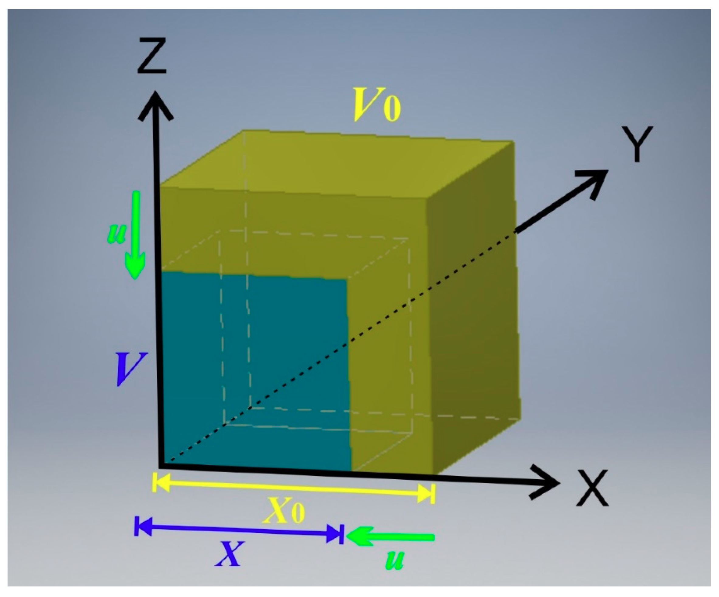
Let us consider a cubic body with edge length $X_0$. Its volume is accordingly $V_0=X_0^3$. This cube is uniformly compressed to edge length $X$ and accordingly to a volume of $V=X^3$ (Figure 1). The edge length before compression is expressed by the reference length and length change, or displacement $u$, as:

$$X_0=X-u$$

(1)

Because of compression, $u<0$.

As mentioned, the change in squared edge length by compression is expanded as:

$$\begin{array}{c}{X}^2-X_0^2=X^2-{\left(X-u\right)}^2=2Xu-u^2\\ X_0^2-X^2=u^2-2Xu\end{array}$$

(2)

Displacement should be proportional to the reference edge length because of uniform compression and is expressed using a proportional constant at a given compression, $c$, as:

$$u=cX$$

(3)

The quantity $c$ is referred to as the strain in the linear elasticity. Using Equation (3), Equation (2) becomes:

$$X^2-X_0^2=2XcX-c^2=\left(2c-c^2\right)X^2$$

(4)

Finite strain in the Eulerian scheme, ${\epsilon }_{\mathrm{E}2}$, is defined as:

$${\epsilon }_{\mathrm{E}2}\equiv c-\frac{1}{2}{c}^2$$

(5)

In this article, finite strain is referred to as the second-power Eulerian strain because it is defined by expanding the second power of length. The change of squared length (Equation (2)) is expressed using the Eulerian finite strain (Equation (5)) as:

$$X^2-X_0^2=2{\epsilon }_{\mathrm{E}2}{X}^2$$

(6)

The ratio of the edge length before compression to the reference edge length is expressed by Eulerian finite strain as:

$$\frac{X_0}{X}={\left(1-2{\epsilon }_{\mathrm{E}2}\right)}^{\frac{1}{2}}$$

(7)

The ratio of the pre-compression volume to the reference volume is also expressed by Eulerian finite strain as:

$$\frac{V_0}{V}={\left(\frac{X_0}{X}\right)}^3={\left(1-2{\epsilon }_{\mathrm{E}2}\right)}^{\frac{3}{2}}$$

(8)

Eulerian finite strain is therefore expressed by the volume ratio as:

$${\epsilon }_{\mathrm{E}2}=\frac{1}{2}\left[1-{\left(\frac{V_0}{V}\right)}^{\frac{2}{3}}\right]$$

(9)

The ε is negative when a body is compressed. To make strain positive by compression, we introduce $f_{\mathrm{E}2}$ as:

$$f_{\mathrm{E}2}=-{\epsilon }_{\mathrm{E}2}=\frac{1}{2}\left[{\left(\frac{V_0}{V}\right)}^{\frac{2}{3}}-1\right]$$

(10)

The quantity $f_{\mathrm{E}2}$ instead of ${\epsilon }_{\mathrm{E}2}$ is usually referred to as Eulerian finite strain.

2.2. The Second-Order Birch–Murnaghan EOS

In isothermal EOSs, pressure, $P$, is expressed as a function of volume, $V$. From thermodynamics, pressure is the volume derivative of Helmholtz energy, $F$, as:

$$P=-{\left(\frac{\partial F}{\partial V}\right)}_T$$

(11)

The Helmholtz free energy of matter should increase with compression and may be expressed by a series of the Eulerian finite strain:

$$F=a_0+a_1{f}_{\mathrm{E}2}+a_2{f_{\mathrm{E}2}}^2+a_3{f_{\mathrm{E}2}}^3+\dots$$

(12)

Because the absolute value of $F$ is arbitrary, the coefficient of the first term in Equation (12) can be $a_0=0$. Because pressure should be zero in an uncompressed state, $f_{\mathrm{E}2}=0$, we have:

$$P_{f_{\mathrm{E}2}=0}=-{\left(\frac{\partial F}{\partial f_{\mathrm{E}2}}\right)}_{T,f_{\mathrm{E}2}=0}{\left(\frac{\partial f_{\mathrm{E}2}}{\partial V}\right)}_{T, f_{\mathrm{E}2}=0}=-a_1{\left(\frac{\partial f_{\mathrm{E}2}}{\partial V}\right)}_{T, f_{\mathrm{E}2}=0}=0$$

(13)

The coefficient of the second term in Equation (12) is therefore $a_1=0$.

Here, we truncate Equation (12) to the ${f_{\mathrm{E}2}}^2$ term for the first approximation and therefore have:

$$F\cong a_2{f}_E{}^2$$

(14)

By substituting Equation (14) into Equation (11), we have

$$P=-{\left\{\frac{\partial }{\partial V}\left(a_2{f}_{\mathrm{E}2}{}^2\right)\right\}}_T=-2a_2{\left(\frac{\partial f_{\mathrm{E}2}}{\partial V}\right)}_T{f}_{\mathrm{E}2}$$

(15)

From the definition of finite strain (Equation (10)), the volume derivative of Eulerian finite strain is:

$${\left(\frac{\partial f_{\mathrm{E}2}}{\partial V}\right)}_T=\frac{\partial }{\partial V}\left[\frac{1}{2}\left\{{\left(\frac{V_0}{V}\right)}^{\frac{2}{3}}-1\right\}\right]=-\frac{1}{3V_0}{\left(\frac{V_0}{V}\right)}^{\frac{5}{3}}$$

(16)

As shown in Appendix A, the coefficient $a_2$ is given by:

$$a_2=\frac{9}{2}{K}_{T_0}{V}_0$$

(17)

where $K_{T_0}$ is the isothermal bulk modulus at standard temperature. By substituting Equations (10), (16), and (17) into Equation (15), we have the second-order Birch-Murnaghan EOS:

$$P=-2\frac{9}{2}{K}_{T_0}{V}_0\frac{1}{2}\left[{\left(\frac{V_0}{V}\right)}^{\frac{2}{3}}-1\right]\left[-\frac{1}{3V_0}{\left(\frac{V_0}{V}\right)}^{\frac{5}{3}}\right]=\frac{3}{2}{K}_{T_0}\left[{\left(\frac{V_0}{V}\right)}^{\frac{7}{3}}-{\left(\frac{V_0}{V}\right)}^{\frac{5}{3}}\right]$$

(18)

This equation contains a subtraction formula between the 7/3 and 5/3 powers of $V_0/V$. The difference of these two powers, 7/3 − 5/3 = 2/3 is owing to the definition of Eulerian finite strain (Equation (10)), and the power of 5/3 in the second term is because of the volume derivative of Eulerian finite strain (Equation (16)).

2.3. The Third-Order Birch–Murnaghan EOS

The concept of the third-order Birch–Murnaghan EOS is almost identical to that of the second-order equation. The difference is that the Helmholtz free energy expressed by the Eulerian finite strain (Equation (12)) is truncated not up to the second term but to the third term as:

$$F\cong a_2{f}_{\mathrm{E}2}{}^2+a_3{f}_{\mathrm{E}2}{}^3$$

(19)

By substituting Equation (19) into Equation (11) and differentiating it with respect to volume, we have:

$$\begin{array}{cc}P=-{\left\{\frac{\partial }{\partial V}\left(a_2{f}_{\mathrm{E}2}{}^2+a_3{f}_{\mathrm{E}2}{}^3\right)\right\}}_T& =-\left(2a_2{f}_{\mathrm{E}2}+3a_3{f}_{\mathrm{E}2}^2\right){\left(\frac{\partial f_{\mathrm{E}2}}{\partial V}\right)}_T\\ & =-2a_2\left(1+{\xi }_1{f}_{\mathrm{E}2}\right){\left(\frac{\partial f_{\mathrm{E}2}}{\partial V}\right)}_T{f}_{\mathrm{E}2}\end{array}$$

(20)

where ${\xi }_1=3a_3/2a_2$. As presented in the Appendix A, the parameter ${\xi }_1$ is given by:

$${\xi }_1=\frac{3}{2}\left(K_{T_0}^{\prime }-4\right)$$

(21)

where $K_{T_0}^{\prime }$ is the pressure derivative of the isothermal bulk modulus at standard temperature. By substituting the definition of Eulerian finite strain (Equation (10)), its volume derivative (Equation (16)), the parameter $a_2$ (Equation (17)), and parameter $m_1$ (Equation (21)) into Equation (20), we have the third-order Birch–Murnaghan EOS as:

$$\begin{array}{c}P=-2\left(\frac{9}{2}{K}_{T_0}{V}_0\right)\left[1+\frac{3}{2}\left(K_{T_0}^{\prime }-4\right)\frac{1}{2}\left\{{\left(\frac{V_0}{V}\right)}^{\frac{2}{3}}-1\right\}\right]\left[-\frac{1}{3V_0}{\left(\frac{V_0}{V}\right)}^{\frac{5}{3}}\right]\frac{1}{2}\left[{\left(\frac{V_0}{V}\right)}^{\frac{2}{3}}-1\right]\\ =\frac{3}{2}{K}_{T_0}\left[{\left(\frac{V_0}{V}\right)}^{\frac{7}{3}}-{\left(\frac{V_0}{V}\right)}^{\frac{5}{3}}\right]\left[1+\frac{3}{4}\left(K_{T_0}^{\prime }-4\right)\left\{{\left(\frac{V_0}{V}\right)}^{\frac{2}{3}}-1\right\}\right]\end{array}$$

(22)

The second term in the first square bracket appears because of the truncation of the Helmholtz free energy to the higher-order (third) term. The form of the curly bracket is owing to the Eulerian finite strain (Equation (10)).

The third-order equation (Equation (22)) becomes identical to the second-order equation (Equation (18)) when

$$K_{T_0}^{\prime }=4$$

(23)

On the other hand, if $K_{T_0}^{\prime }$ is neglected as $K_{T_0}^{\prime }=0$, the third-order equation should differ from the second-order equation.

2.4. The Fourth-Order Birch–Murnaghan EOS

For the fourth-order EOS, Equation (12) is truncated up to the fourth term as:

$$F\cong a_2{f}_{\mathrm{E}2}{}^2+a_3{f}_{\mathrm{E}2}{}^3+a_4{f}_{\mathrm{E}2}{}^4$$

(24)

The pressure is then expressed as:

$$P=-\left(2a_2{f}_{\mathrm{E}2}+3a_3{f}_{\mathrm{E}2}^2+a_4{f}_{\mathrm{E}2}{}^3\right){\left(\frac{\partial f_{\mathrm{E}2}}{\partial V}\right)}_T=-2a_2{f}_{\mathrm{E}2}\left(1+{\xi }_1{f}_{\mathrm{E}2}+{\xi }_2{f}_{\mathrm{E}2}^2\right){\left(\frac{\partial f_{\mathrm{E}2}}{\partial V}\right)}_T$$

(25)

where ${\xi }_2=2a_4/a_2$. As given in the Appendix A, the parameter ${\xi }_2$ is:

$${\xi }_2=\frac{9K_{T_0}^{\prime }{}^2-63K_{T_0}^{\prime }+9K_{T_0}{K}_{T_0}^{″}+143}{6}$$

(26)

where $K_{T_0}^{″}$ is the second pressure derivative of the isothermal bulk modulus at standard temperature.

Similar to the lower-order EOSs, we have the fourth-order Birch–Murnaghan EOS as:

$$\begin{array}{c}P=\frac{3}{2}{K}_{T_0}\left[{\left(\frac{V_0}{V}\right)}^{\frac{7}{3}}-{\left(\frac{V_0}{V}\right)}^{\frac{5}{3}}\right][1+\frac{3}{4}\left(K_{T_0}^{\prime }-4\right)\left\{{\left(\frac{V_0}{V}\right)}^{\frac{2}{3}}-1\right\}\\ +\frac{1}{24}\left(9K_{T_0}^{\prime }{}^2-63K_{T_0}^{\prime }+9K_{T_0}{K}_{T_0}^{″}+143\right){\left\{{\left(\frac{V_0}{V}\right)}^{\frac{2}{3}}-1\right\}}^2]\end{array}$$

(27)

This fourth-order equation (Equation (27)) becomes identical to the third-order equation when

$$K_{T_0}^{″}=-\frac{1}{9K_{T_0}}\left(9K_{T_0}^{\prime }{}^2-63K_{T_0}^{\prime }+143\right)$$

(28)

Again, if $K_{T_0}^{″}$ is neglected as $K_{T_0}^{″}=0$, the fourth-order equation should differ from the third-order equation.

3. Equations of States from Other Finite Strain Definitions

Through deriving the Birch–Murnaghan EOS, we may have some questions in mind. One is why the Eulerian scheme is more frequently used to describe the compression of bodies instead of the Lagrangian scheme. Another question is why is a change in squared length considered; why not other powers of length? Murnaghan’s [1] argument leaves one to reflect that the use of squared length was based on Pythagorean theorem but there is no physical reason. To answer these questions, we derive EOSs from finite strain using the following different definitions:

• Lagrangian scheme, expansion of squared length, referred to as the second-power Lagrangian EOS;
• Eulerian scheme, linear expansion of length, referred to as the first-power Eulerian EOS;
• Eulerian scheme, expansion of cubed length, referred to as the third-power Eulerian EOS.

3.1. The Second-Power Lagrangian EOS

Let us come back to Figure 1. In the Lagrangian scheme, the reference is taken as the pre-compressed state. Hence, the length after compression, $X$, is expressed using the reference length, $X_0$, and displacement:

$$X=X_0+u$$

(29)

The change in squared edge length is:

$$X^2-X_0^2=2X_{0}u+u^2$$

(30)

The displacement is expressed by the reference length as:

$$u=c_0{X}_0$$

(31)

Note that Equation (31) differs from Equation (3) unless $X\cong X_0$, namely when strain is finite.

Using Equation (31), Equation (30) becomes:

$$X^2-X_0^2=\left(2c_0+c_0{}^2\right)X_0^2$$

(32)

We now define the Lagrangian finite strain, ${\epsilon }_{\mathrm{L}2}$, as:

$${\epsilon }_{\mathrm{L}2}\equiv c_0+\frac{1}{2}{c}_0{}^2$$

(33)

Like the Eulerian scheme, Lagrangian finite strain is expressed using the volume ratio:

$${\epsilon }_{\mathrm{L}2}=\frac{1}{2}\left[{\left(\frac{V}{V_0}\right)}^{\frac{2}{3}}-1\right]$$

(34)

For convenience, the quantity $f_{\mathrm{L}2}$ below is hereafter referred to as the second-power Lagrangian finite strain:

$$f_{\mathrm{L}2}=-{\epsilon }_{\mathrm{L}2}=\frac{1}{2}\left[1-{\left(\frac{V}{V_0}\right)}^{\frac{2}{3}}\right]$$

(35)

EOSs are constructed based on this strain, which is hereafter referred to as the second-power Lagrangian EOS. The Birch–Murnaghan EOS is hereafter referred to as the second-power Eulerian EOS.

Like the second-order second-power Eulerian EOS, the Helmholtz free energy is expressed with the second-power Lagrangian finite strain squared as:

$$F\cong a_2{f}_{\mathrm{L}2}{}^2$$

(36)

The expression for pressure in the Lagrangian scheme is identical to the Eulerian scheme as:

$$P=-2a_2{f}_{\mathrm{L}2}{\left(\frac{\partial f_{\mathrm{L}2}}{\partial V}\right)}_T$$

(37)

The volume derivative of the second-power Lagrangian finite strain is given by:

$${\left(\frac{\partial f_{\mathrm{L}2}}{\partial V}\right)}_T=-\frac{1}{3V_0}{\left(\frac{V}{V_0}\right)}^{-\frac{1}{3}}$$

(38)

The formula of parameter $a_2$ in the Lagrangian scheme is identical to that in the Eulerian scheme (Equation (17)). As a result, the second-order second-power Lagrangian EOS is given by:

$$P=\frac{3}{2}{K}_{T_0}\left[{\left(\frac{V}{V_0}\right)}^{-\frac{1}{3}}-{\left(\frac{V}{V_0}\right)}^{\frac{1}{3}}\right]=\frac{3}{2}{K}_{T_0}\left[{\left(\frac{V_0}{V}\right)}^{\frac{1}{3}}-{\left(\frac{V_0}{V}\right)}^{-\frac{1}{3}}\right]$$

(39)

For the third-order EOS, the Helmholtz free energy is expanded to the third term of $f_{\mathrm{L}2}$ as:

$$F\cong a_2{f}_{\mathrm{L}2}{}^2+a_3{f}_{\mathrm{L}2}{}^3$$

(40)

By differentiating Equation (33) with respect to volume, pressure is expressed as:

$$P=-2a_2\left(1+{\xi }_1{f}_{\mathrm{L}2}\right){\left(\frac{\partial f_{\mathrm{L}2}}{\partial V}\right)}_T{f}_{\mathrm{L}2}$$

(41)

The expression of $m_1$ for the second-power Lagrangian finite strain differs from that for the second-power Eulerian strain and is given by:

$${\xi }_1=\frac{3}{2}{K_{T_0}}^{\prime }$$

(42)

From Equations (17), (28), (34), and (35), we have the third-order second-power Lagrangian EOS as:

$$P=\frac{3}{2}{K}_{T_0}\left[{\left(\frac{V}{V_0}\right)}^{-\frac{1}{3}}-{\left(\frac{V}{V_0}\right)}^{\frac{1}{3}}\right]\left[1+\frac{3}{4}{K}_{T_0}^{\prime }\left\{1-{\left(\frac{V}{V_0}\right)}^{\frac{2}{3}}\right\}\right]$$

(43)

The third-order equation (Equation (43)) becomes identical to the second-order equation (Equation (39)) when:

$$K_{T_0}^{\prime }=0$$

(44)

In contrast to the Eulerian scheme, the neglect of $K_{T_0}^{\prime }$ as $K_{T_0}^{\prime }=0$ is identical to the neglect of a term higher than third order in the Helmholtz free energy (Equation (36)).

3.2. Finite Strains and EOSs from Linear Length

The change of length itself, namely the first power of length, is considered here in the Eulerian scheme and given from Equations (1) and (3) as:

$$X-X_0=u=cX$$

(45)

The first-power Eulerian strain, $f_{\mathrm{E}1}$, is therefore defined as:

$$f_{\mathrm{E}1}\equiv -{\epsilon }_{\mathrm{E}1}=-c$$

(46)

Similar to the change in squared length, the first-power Eulerian strain is expressed by the volume change $V_0/V$ as:

$$f_{\mathrm{E}1}=\left[{\left(\frac{V_0}{V}\right)}^{\frac{1}{3}}-1\right]$$

(47)

The volume derivative of the first-power Eulerian finite strain is given by:

$${\left(\frac{\partial f_{\mathrm{E}1}}{\partial V}\right)}_T=-\frac{1}{3V_0}{\left(\frac{V_0}{V}\right)}^{\frac{4}{3}}$$

(48)

The parameter $a_2$ for the first-power Eulerian strain is identical to those of the second-power strain in the Eulerian and Lagrangian schemes. The second-order first-power Eulerian EOS is, therefore, given by:

$$P=K_{T_0}\left[{\left(\frac{V_0}{V}\right)}^{\frac{5}{3}}-{\left(\frac{V_0}{V}\right)}^{\frac{4}{3}}\right]$$

(49)

The parameter ${\xi }_1$ is given by:

$${\xi }_1=\frac{3}{2}\left(K_{T_0}^{\prime }-3\right)$$

(50)

The third-order first-power Eulerian EOS is therefore given by:

$$P=3K_{T_0}\left[{\left(\frac{V_0}{V}\right)}^{\frac{5}{3}}-{\left(\frac{V_0}{V}\right)}^{\frac{4}{3}}\right]\left[1+\frac{3}{2}\left(K_{T_0}^{\prime }-3\right)\left\{{\left(\frac{V_0}{V}\right)}^{\frac{1}{3}}-1\right\}\right]$$

(51)

3.3. Finite Strains and EOSs from Cubed Length

We now consider the change in length cubed, namely the third-power of length in the Eulerian scheme, which is given from Equations (1) and (3) as:

$$X^3-X_0^3=\left(3c-3c^2+c^3\right)X^3$$

(52)

The third-power Eulerian strain, $f_{\mathrm{E}3}$, is therefore defined as:

$$f_{\mathrm{E}3}\equiv -{\epsilon }_{\mathrm{E}3}=-c+c^2-\frac{1}{3}{c}^3$$

(53)

Similar to those with the change in squared length, the first-power Eulerian strain is expressed by volume change $V_0/V$:

$$f_{\mathrm{E}3}=\frac{1}{3}\left[\left(\frac{V_0}{V}\right)-1\right]$$

(54)

The volume derivative of the third-power Eulerian finite strain is given by:

$${\left(\frac{\partial f_{\mathrm{E}3}}{\partial V}\right)}_T=-\frac{1}{3V_0}{\left(\frac{V_0}{V}\right)}^2$$

(55)

In the same way as shown previously, the second-order third-power Eulerian EOS is given by:

$$P=K_{T_0}\left[{\left(\frac{V_0}{V}\right)}^3-{\left(\frac{V_0}{V}\right)}^2\right]$$

(56)

The parameter ${\xi }_1$ is given by:

$${\xi }_1=\frac{3}{2}\left(K_{T_0}^{\prime }-5\right)$$

(57)

The third-order third-power Eulerian EOS is therefore given by:

$$P=K_{T_0}\left[{\left(\frac{V_0}{V}\right)}^3-{\left(\frac{V_0}{V}\right)}^2\right]\left[1+\frac{1}{2}\left(K_{T_0}^{\prime }-5\right)\left\{\frac{V_0}{V}-1\right\}\right]$$

(58)

4. Discussion

4.1. Comparison of Birch–Murnaghan EOSs of Different Orders

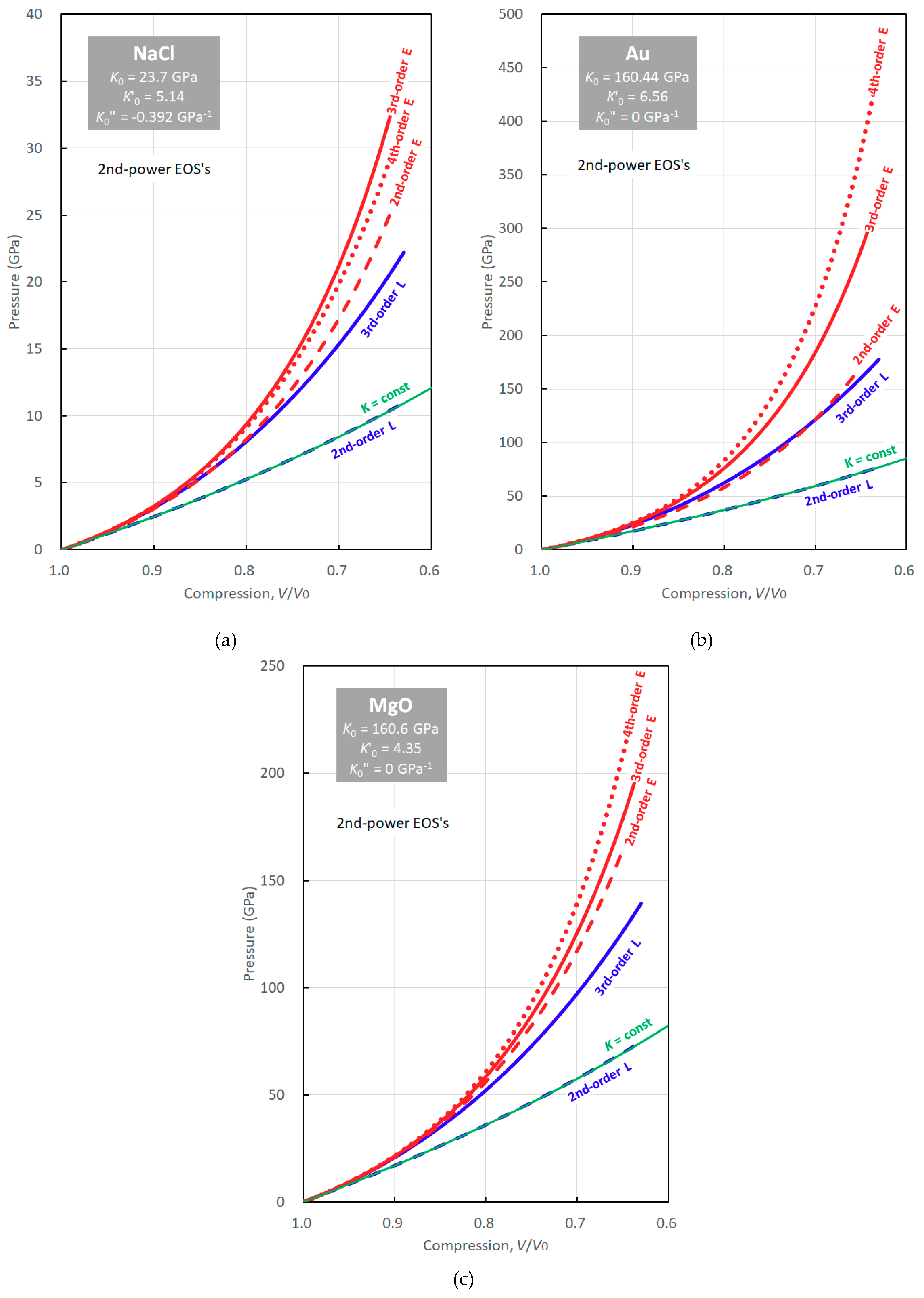
Figure 2 shows pressures obtained by the second-, third- and fourth-order Birch–Murnaghan EOSs of NaCl in the B1-structure, Au, and MgO, which are materials frequently used as pressure standards in high-pressure experiments. The isothermal bulk moduli of these three materials and their first and second pressure derivatives at ambient temperature and zero pressure used for construction of Figure 2 are summarized in

Table 1. Bulk moduli and their pressure derivatives of frequently used pressure standard materials.

Material	${\mathit{K}}_{{\mathit{T}}_0}\left(\mathbf{GPa}\right)$	${{\mathit{K}}_{{\mathit{T}}_0}}^{\prime }$	${{\mathit{K}}_{{\mathit{T}}_0}}^{\prime \prime }\left({\mathbf{GPa}}^{-1}\right)$	Reference
NaCl	23.7	5.14	−0.392	[5]
Au	160.44	6.56	0	[6]
MgO	160.64	4.35	0	[7]

. Note that these EOS parameters were all obtained by the latest studies of sound velocity measurements [5,6,7].

The second- and third-order Birch–Murnaghan EOSs give significantly different pressures for NaCl and Au under high compression owing to large deviations of ${K_{T_0}}^{\prime }$ from 4 (5.14 and 6.56). At $V/V_0=0.75$, the second- and third-order EOSs yield 12.1 and 14.3 GPa for NaCl and 85 and 112 GPa for Au, respectively, with differences of 18% and 41% in these cases. Birch [8] justified the validity of the Birch-Murnaghan EOS by identifying the second- and third-order EOSs within experimental uncertainty (e.g., ${K_{T_0}}^{\prime }\cong 4$). However, modern experimental results have demonstrated that ${K_{T_0}}^{\prime }\cong {K_{S_0}}^{\prime }$ and significantly differs from 4 in many materials (see Table 11 in Bass [9]), which therefore compromises the validity of the second-order Birch–Murnaghan EOS.

Figure 2a also shows that the fourth-order equation gives slightly lower pressures than the third-order equation in the case of NaCl. At $V/V_0=0.75$, the fourth-order equation gives a pressure of 13.7 GPa, which is about 4% lower than that from the third-order equation. For the third- and fourth-order equations to give identical pressures, the second pressure derivative of the isothermal bulk modulus must not be ${K_{T_0}}^{″}=-0.392$ GPa⁻¹ but rather ${K_{T_0}}^{″}=-0.267$ GPa⁻¹. Figure 2b,c also show the fourth-order Birch–Murnaghan EOSs of Au and MgO whose second pressure derivatives of the isothermal bulk modulus at zero pressure are set to ${K_{T_0}}^{″}=0$. The pressure at the bottom of the Earth’s mantle is 136 GPa. To obtain such pressure by the third-order Birch–Murnaghan EOSs of Au and MgO, the compression must be $V/V_0=0.736$ and $V/V_0=0.678$, respectively. Under these compressions, the fourth-order Birch–Murnaghan EOSs with ${K_{T_0}}^{″}=0$ give 160 and 152 GPa. Thus, approximations that ignore higher-order terms of finite strain and equate higher-order derivatives of the isothermal bulk modulus to zero are not identical in the Birch–Murnaghan EOSs.

The differences in pressure given by the two kinds of EOSs above correspond to 470 and 330 km in the case of Au and MgO, respectively. The depth of the mantle phase transition at the base of the Earth’s mantle is particularly complicated to argue. Although Hirose et al. [10] determined the post-spinel transition boundary in MgSiO₃ using Au and MgO pressure scales to interpret the phase boundary pressure as the D” layer, their argument contains errors on the order of a few hundred km simply by neglecting $K_{T_0}^{\prime }$ as ${K_{T_0}}^{″}=0$.

4.2. Eulerian Versus Lagrangian Schemes

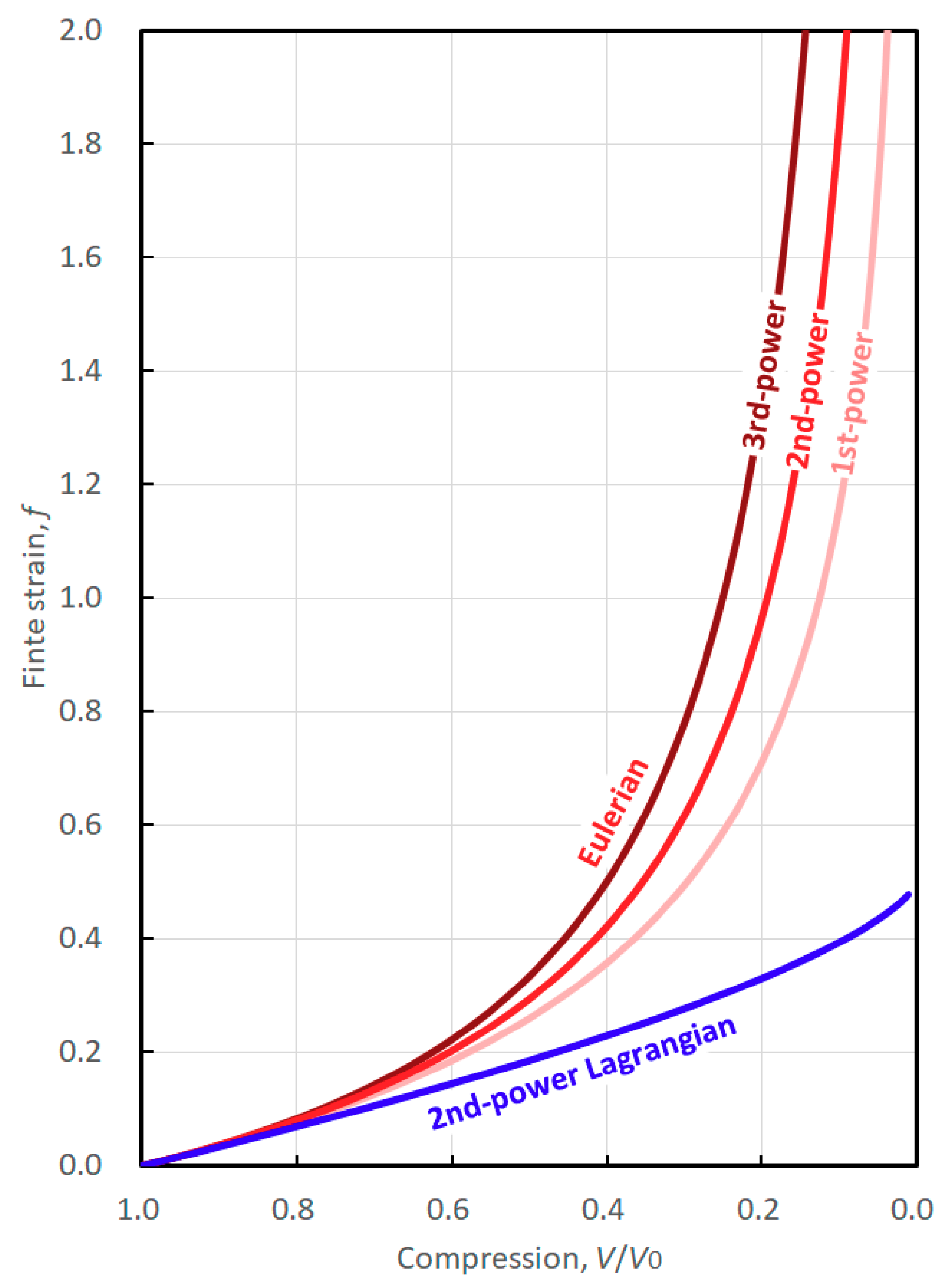
An essential difference between the Eulerian and Lagrangian finite strains is that the volume ratio is inversed with respect to one another (Equations (10) and (35)). Because the reference state is before compression in the Lagrangian scheme, the post-compression volume is put in the numerator of the strain formula (Equation (35)). As shown in Figure 3, the Lagrangian finite strain increases nearly linearly upon compression to $V/V_0=0.2$ and then approaches a finite value (0.5) with further compression ($V/V_0\to 0$). As a result, the Helmholtz free energy and its volume derivative, namely pressure, only moderately increase with compression. However, it is important to note that pressure approaches infinity with compression to zero volume because the volume derivative of the finite strain and one term of the EOS are proportional to the −1/3 power of $V/V_0$ (Equations (38), (39), and (43)).

In contrast to the Lagrangian scheme, the Eulerian reference state is after compression and the post-compression volume is put in the denominator of the strain formula (Equation (10)). As shown in Figure 3, all Eulerian finite strains rapidly increase and then diverge to infinity as $V/V_0\to 0$. As a result, the Helmholtz free energy and pressure also rapidly increase to infinity with $V/V_0\to 0$. This behavior in the Eulerian scheme is in better agreement than that in the Lagrangian scheme. It is also important to note that the rate of pressure increase is very similar in both schemes under low compression. In other words, both schemes give the same results if the strain is infinitesimal.

Figure 2a–c show pressures given by the second- and third-order (second-power) Lagrangian EOSs as well as the Eulerian EOS’s. For comparison, we also show pressures given by the simplest EOS, which is obtained by integrating the definition of the isothermal bulk modulus as:

$$P=K_{T_0}\ln \left(\frac{V_0}{V}\right)$$

(59)

with green curves in Figure 2a–c.

As previously discussed, finite strains given in the Eulerian scheme increase much more rapidly with compression than those of the Lagrangian scheme. The second-order second-power Lagrangian EOS gives almost identical pressures as the integration of a constant bulk modulus (Equation (37)). This means that the second-order Lagrangian EOS gives pressures without considering an increase in bulk modulus with compression. This is reasonable because the third-order Lagrangian EOS becomes identical to the second-order Lagrangian EOS when $K_{T_0}^{\prime }$ is neglected as $K_{T_0}^{\prime }=0$. In contrast, the Eulerian EOSs give substantially higher pressures than when integrating a constant bulk modulus (Equation (59)). As can be seen from the fact that the second- and third-order (second-power) Eulerian EOSs become identical in the case of $K_{T_0}^{\prime }=4$, the Eulerian EOSs implicitly contain the effects of an increased bulk modulus with compression.

The EOSs in both schemes converge with increasing order owing to better approximations of the Helmholtz free energy by the finite strains. This is the case for MgO (Figure 2c), however not for Au (Figure 2b). The small difference between the third- and fourth-orders of EOSs of NaCl (Figure 2a) does not imply that expansion to higher orders effectively helps conversion of the two schemes. These observations imply an essential problem with the Lagrangian scheme.

4.3. Equations of State Obtained from Expansions of Different Powers of Length

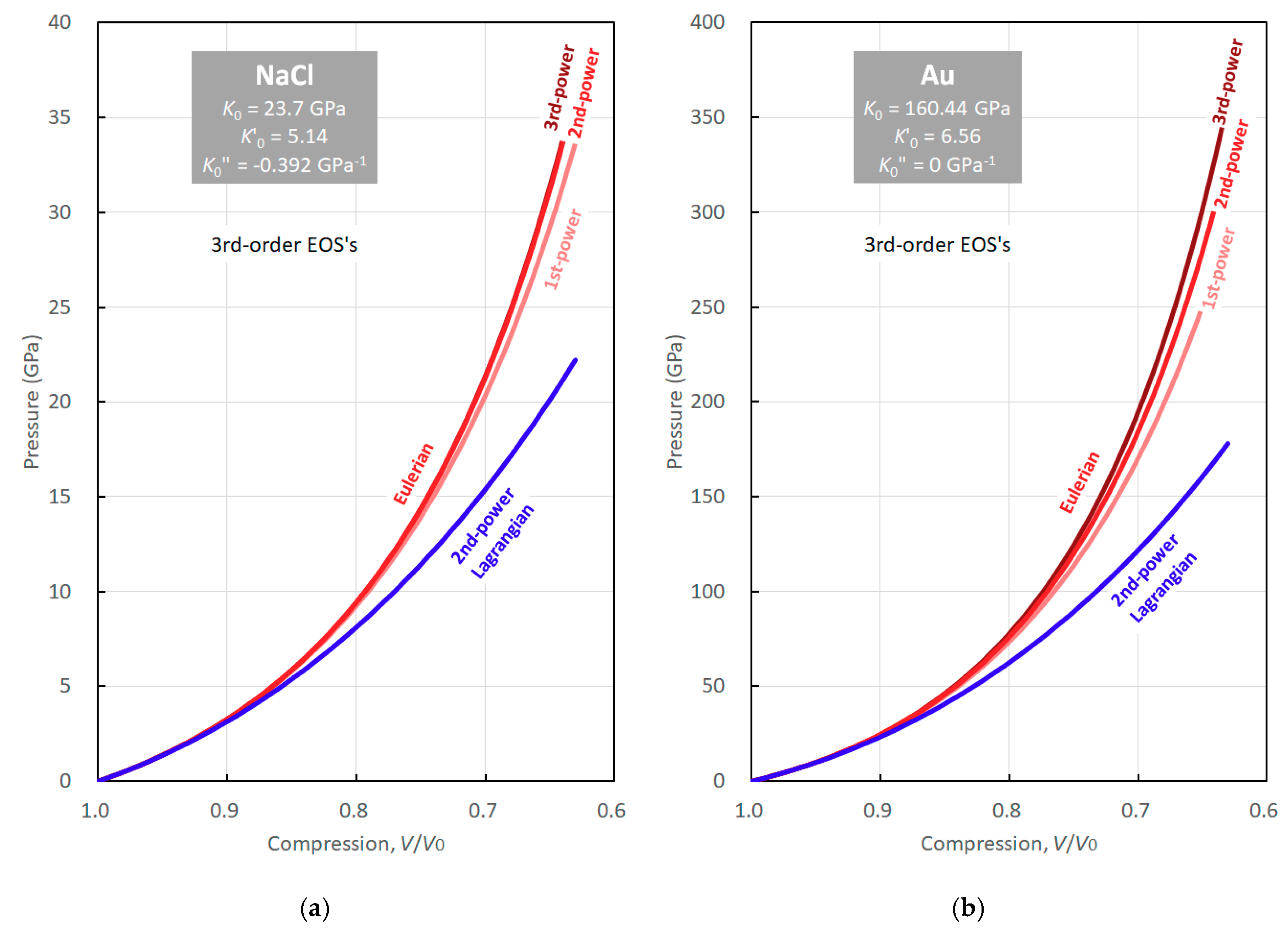
Figure 4a–c, show the third-order EOSs of NaCl, Au, and MgO, respectively, based on Eulerian finite strain defined by expansion of the first- (linear), second- (squared) and third- (cubed) powers of length given by Equations (22), (51), and (58), respectively. The EOS from the expansion of the second-power of length is the Birch–Murnaghan EOS. Because the finite strains based on higher powers of length increase more rapidly with compression, the EOSs based on higher powers of length are expected to give higher pressures. This is the case for materials with high K” such as Au. As is seen in Figure 4b, the first-, second- and third-power EOSs of Au gives pressures of 73, 76, and 78 GPa at $V/V_0=0.8$, respectively. The differences of the first- and third-power EOSs from the Birch–Murnaghan (second-power) EOS are both about −4% and +3%. The discrepancy between different powers of EOSs increases with compression, giving pressures of 170, 184, and 194 GPa, respectively, with differences of about −8% and +5%. The finite strains more rapidly increase under compression with increasing power of $V_0/V$ from 1/3 to 2/3 and then to 1 (Equations (10), (47), and (54)), as shown in Figure 3. Because these three EOSs are obtained in the same way except for the power of length to define the finite strain, we cannot say that the Birch–Murnaghan EOS provides substantially more accurate pressures than the others.

As discussed previously, Birch [8] justified the Birch–Murnaghan EOSs by the identity of the second- and third-order EOSs when ${K_{T_0}}^{\prime }\cong 4$, which is approximately the case in many kinds of materials. As Equations (51) and (58) show, the second- and third-order Eulerian EOSs based on finite strains defined from the first- and third-powers of length become identical when $K_{T_0}^{\prime }=3$ and $K_{T_0}^{\prime }=5$, respectively. Again, as summarized by Bass [9], the $K_{T_0}^{\prime }$ of the majority of solids are larger than 4. In the case of Au, $K_{T_0}^{\prime }=6.56$ and the third-power EOS (Equation (58)) should therefore be more appropriate for Au than the Birch–Murnaghan EOS (Equation (22)) if we follow Birch’s [8] justification.

4.4. Examination of Equations of State Using Pressure Scale-Free Experimental Data

In this section, we examine the validity of the second-power Lagrangian and first- and third-power Eulerian third-order EOS’s in comparison with the third-order Birch–Murnaghan (second-power Eulerian) EOS. Specifically, we attempt to obtain parameters of the Mie-Grüneisen-Debye thermal EOS of MgO on the basis of these isothermal EOSs using pressure scale-free experimental data following the method by Tange et al. [11]. “Pressure scale-free” data were data that can be used to build an equation of state, but no other pressure scales such as pressure values obtained using equations of state of other pressure standard materials were used to obtain those data. Use of pressure scale-free data allows us building an equation of state with avoiding any circular argument. The pressure scale-free experimental data sets used here are zero-pressure and high-temperature thermal expansivity, zero-pressure and high-temperature adiabatic bulk moduli, 300-K and compressed adiabatic bulk moduli, and shock compression. Data sources are summarized in Table 2 of Tange et al. [11]. The following parameters at 300 K and 0 GPa are fixed: lattice volume, adiabatic bulk modulus, thermal expansivity, and isobaric heat capacity. The parameters obtained by these fittings are given in Table 3 of Tange et al. [11]. Note that parameters $a$ and $b$ are adjustable to express the volume dependence of the Grüneisen parameter $\gamma$, according to the following formula:

$$\gamma \left(V\right)={\gamma }_0\left\{1+a\left[{\left(\frac{V}{V_0}\right)}^b-1\right]\right\}$$

(60)

Table 2. Parameters obtained by fitting pressure-scale-free data to various EOSs.

Parameter	2nd-Power Eulerian EOS (Birch-Murnaghan)	2nd-Power Lagrangian EOS	1st-Power Eulerian EOS	3rd-Power Eulerian EOS
$V_0$ (Å3)	74.698 (fixed)	74.698 (fixed)	74.698 (fixed)	74.698 (fixed)
$K_{T_0}$ (GPa)	160.64	160.55	160.64	160.63
$K_{T_0}^{\prime }$	4.221	4.909	4.293	4.347
${\theta }_0$ (K)	761	761 (fixed)	761 (fixed)	761 (fixed)
${\gamma }_0$	1.431	1.496	1.436	1.440
$a$	0.29	0 (fixed)	0.20	0.14
$b$	3.5		4.4	5.5

$V_0$: lattice volume at 300 K and 0 GPa; $K_{T_0}$: isothermal bulk modulus; $K_{T_0}^{\prime }$: pressure derivative of the bulk modulus; ${\theta }_0$: Debye temperature; ${\gamma }_0$: Grüneisen parameter; a, b: parameters to express volume dependence of the Grüneisen parameter given in Equation (59).

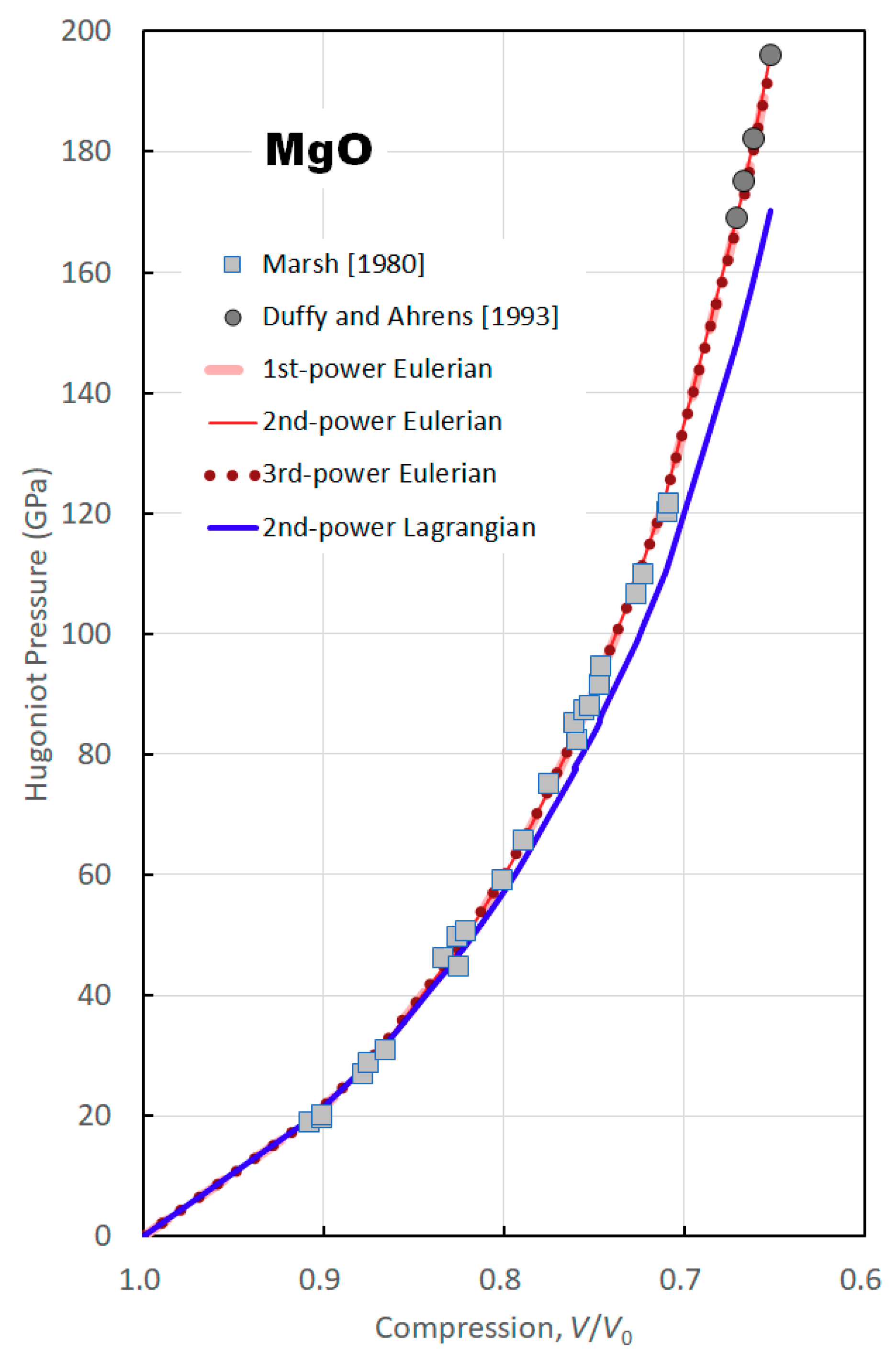
lists the obtained parameters of the thermal EOSs and Figure 5 shows the reproduction of Hugoniot curves using the obtained parameters.

Figure 5 indicates that all Eulerian EOSs provide Hugoniot curves in agreement with the experimental data by Marsh [12] and Duffy and Ahrens [13], whereas the Lagrangian EOS does not. The reason for the failure in construction of an EOS in the Lagrangian scheme is that the parameters $a$ and $b$ in Equation (60) must not be less than zero; namely, thermal pressure or thermal expansivity should not increase with increasing pressure. Because the Lagrangian EOS gives much lower pressures at ambient temperature than the Eulerian EOSs, the thermal pressure must be abnormally high in the Lagrangian scheme to reproduce the shock experiment data. As a conclusion, the Eulerian scheme is more appropriate than the Lagrangian scheme to construct an EOS of real materials. On the other hand, linear and cubed length expansions in the Eulerian scheme provide equivalently appropriate EOSs compared with the EOS derived from the squared length expansion to define finite strain.

References

- Murnaghan, F.D. Finite Deformations of an Elastic Solid. Am. J. Math. 1937, 59, 235–260. [Google Scholar] [CrossRef]
- Birch, F. Finite elastic strain of cubic crystals. Phys. Rev. 1947, 71, 809–824. [Google Scholar] [CrossRef]
- Poirier, J.P. Introduction to the Physics of the Earth’s Interior, 2nd ed.; Cambridge University Press: Cambridge, UK, 2000; p. 312. [Google Scholar]
- Anderson, O.L. Equations of States of Solids for Geophysics and Ceramics Science; Oxford University Press: New York, NY, USA, 1995; p. 405. [Google Scholar]
- Matsui, M.; Higo, Y.; Okamoto, Y.; Irifune, T.; Funakoshi, K. Simultaneous sound velocity and density measurements of NaCl at high temperatures and pressures: Application as a primary pressure standard. Am. Mineral 2012, 97, 670–1675. [Google Scholar] [CrossRef]
- Song, M.; Yoneda, A. Ultrasonic measurements of single-crystal gold under hydrostatic pressures up to 8 GPa in a Kawai-type multi-anvil apparatus. Chin. Sci. Bull. 2008, 52, 1600–1606. [Google Scholar] [CrossRef]
- Kono, Y.; Irifune, T.; Higo, Y.; Inoue, T.; Barnhoorn, A. P-V-T relation of MgO derived by simultaneous elastic wave velocity and in situ X-ray measurements: A new pressure scale for the mantle transition region. Phys. Earth Planet. Inter. 2010, 183, 196–211. [Google Scholar]
- Birch, F. Elasticity and constitution of the earth’s interior. J. Geophys. Res. 1952, 57, 227–286. [Google Scholar] [CrossRef]
- Bass, J.D. Elasticity of Minerals, Glasses, and Melts. Miner. Phys. Crystallogr. Handb. Phys. Constants 1995, 2, 45–63. [Google Scholar]
- Hirose, K.; Sinmyo, R.; Sata, N.; Ohishi, Y. Determination of post-perovskite phase transition boundary in MgSiO3 using Au and MgO pressure standards. Geophys. Res. Lett. 2006, 33, L0310. [Google Scholar] [CrossRef]
- Tange, Y.; Nishihara, Y.; Tsuchiya, T. Unified analyses for P-V-T equation of state of MgO: A solution for pressure-scale problems in high P-T experiments. J. Geophys. Res. Solid Earth 2009, 114, B03208. [Google Scholar] [CrossRef]
- Marsh, S.P. LASL Shock Hugoniot Data; University California Press: Berkeley, CA, USA, 1980; pp. 312–313. [Google Scholar]
- Duffy, T.S.; Ahrens, T.J. Thermal expansion of mantle and core materials at very high pressure. Geophys. Res. Lett. 1993, 20, 1103–1106. [Google Scholar] [CrossRef] [Green Version]
Figure 1.
Finite uniform compression of a cube. The initial edge length of the cube is reduced to the final edge length . The volume of the cube accordingly decreases from to .
Figure 2.
Comparison of the second-, third- and fourth-order Birch–Murnaghan equations of state (EOSs). (a) NaCl (B1) data are from Matsui et al. [5]; (b) Au data are from Song and Yoneda [6]; (c) MgO data are from Kono et al. [7]. Red and blue colors denote the Eulerian and Lagrangian schemes, respectively. The dashed, solid, and dotted curves are of the second-, third- and fourth-order EOSs, respectively. The green solid curve denotes the pressure-volume relation obtained by integration of the definition of the bulk modulus (Equation (59)).
Figure 3.
Comparison of the Eulerian and Lagrangian finite strains derived by expansion of the powered length as a function of compression . The light red, red, and dark red curves denote the finite strains by expansion of the linear, squared, and cubed lengths in the Eulerian scheme, respectively, and the blue curve denotes those of the squared lengths in the Lagrangian scheme.
Figure 4.
Pressures given by the second- (light red), third- (red) and fourth- (dark red) power Eulerian and the second-power Lagrangian (blue) third-order EOSs. (a) NaCl; (b) Au; (c) MgO.
Figure 5.
Hugoniot curves of MgO reproduced by the various EOSs using pressure scale-free data following Tange et al. [11]. The dashed light-red, thin-solid red, dotted dark-red, and solid blue curves are obtained from the first-, second- and fourth- Eulerian and second-power Lagrangian EOSs, respectively. The light-gray square and dark-gray circle are experimental data obtained by Marsh [12] and Duffy and Ahrens [13], respectively.