

Surface Pencil Couple with Bertrand Couple as Joint Principal Curves in Galilean 3-Space

1
Department of Mathematics, Science and Arts College, King Abdulaziz University, Rabigh 21911, Saudi Arabia
2
Department of Mathematics, Faculty of Science, University of Assiut, Assiut 71516, Egypt
*
Author to whom correspondence should be addressed.
†
These authors contributed equally to this work.
Axioms 2023, 12(11), 1022; https://doi.org/10.3390/axioms12111022
Submission received: 13 September 2023
/
Revised: 25 October 2023
/
Accepted: 28 October 2023
/
Published: 30 October 2023
(This article belongs to the Special Issue Differential Geometry and Its Application II)
Abstract
:A principal curve on a surface plays a paramount role in reasonable implementations. A curve on a surface is a principal curve if its tangents are principal directions. Using the Serret–Frenet frame, the surface pencil couple can be expressed as linear combinations of the components of the local frames in Galilean 3-space . With these parametric representations, a family of surfaces using principal curves (curvature lines) are constructed, and the necessary and sufficient condition for the given Bertrand couple to be the principal curves on these surfaces are derived in our approach. Moreover, the necessary and sufficient condition for the given Bertrand couple to satisfy the principal curves and the geodesic requirements are also analyzed. As implementations of our main consequences, we expound upon some models to confirm the method.
MSC:
53A04; 53A05; 53A171. Introduction
Principal curve is designated as one of the significant curves on a surface and it plays a primary role in differential geometry [1,2,3,4]. It is an advantageous gadget in surface examination for showing contrast of the principal direction. The harmonic principal curvature and principal curves are considerable and associated with the smooth surfaces. Principal curves can direct the realization of surfaces, quietly utilized in geometric designing, and can constitute consistency, surface polygonization, and surface fulfillment. There exists an enormous literature on the topic, including various monographs, for instance: Martin [5] studied systematic surface patches restricted by principal curves, which are named principal patches. Martin presented that the presence of such patches was conditioned upon confirmed situations corresponding on the patch border curves. Alourdas et al. [6] addressed a mode to confirm a net principal curves on a B-spline surface. Maekawa et al. [7] extended a style to take out the generic characteristics of free-shape parametric surfaces for form inspection. They researched the generic advantage of the umbilics and attitude principal curves that go through an umbilic on a parametric free-shape surface. Che and Paul [8] expanded a manner to resolve and calculate the principal curves and their geometric properties specified on an implicit surface. They also offered a new standard for non-umbilical points and umbilical points on an implicit surface. Zhang et al. [9] proved a planner for calculating and envisaging the principal curves pointed on an implicit surface. Kalogerakis et al. [10] derived a powerful substructure for establishing principal curves by point clouds. Their approach is reasonable for surfaces of random genus, with or without borderlines, and is statistically powerful to use with outliers maintaining surface characteristics. They found the approach to be efficient through an area of synthetic and real-world input data collections with changing amounts of noise and outliers. In practical uses, however, crucial work has focused on the backward exploration or reverse issue: given a 3D curve, how can we locate those surfaces that are faced with this curve as a distinctive curve, if possible, rather than locating and furnishing curves on analytical curved surfaces? Wang et al. [11] was the first to handle the issue of assembling a surface family with a designated locative geodesic curve, through which every surface can be a candidate for mode style. They demonstrated the necessary and sufficient conditions for the coefficients to be satisfied with both the isoparametric and the geodesic demands. This scheme has been used by many scholars (see, for example, [12,13,14,15,16,17,18,19,20,21,22,23]).
Galilean geometry is the simplest pattern of a semi-Euclidean geometry for which the isotropic cone reduces to a plane. It is indicated as a bridge from Euclidean geometry to special relativity. The main spine of Galilean geometry is its private gravity, that is, it allows the scientist to search it in detail without using large amounts of time and energy. In other words, the view of Galilean geometry shapes its development with an unpretentious question, and a gross stretch of a modern geometric community is crucial for its efficient comparison with Euclidean geometry. Also, aggregate evolution is practical to supply the scientist with the psychological emphasis of the uniformity of the inspected structure [24,25]. In the (three-dimensional) Galilean space , there are several studies dealing with , for example, Dede et al. [26,27] resolved tub surfaces, the descriptions of the parallel surfaces. Yuzbasi et al. [28,29] considered a surface family with a curve to be a joint asymptotic curve and geodesic. Jiang et al. [30] considered surface pencil couple with Bertrand couple as joint asymptotic curves. Almoneef and Abdel-Baky [31] designed a surface family with Bertrand curves to be geodesic curves. AL-Jedani and Abdel-Baky [32] considered the surface family and developable surface family with a joint geodesic curve, respectively.
It is known that on any surface there are three main kinds of curves: principal curves (curvature lines), asymptomatic curves, and geodesic curves. In [30], the study focused on how to construct family surfaces via Bertrand curves that are asymptomatic, whereas our work addresses a very new idea related to a differential geometry field based on construction of a family of surfaces using principal curves (curvature lines). Ref. [31] investigated a similar idea but used the geodesic curves instead of principal ones. In addition, a team of researchers, referred to as Li et al. and cited in [32,33,34,35,36,37,38,39,40,41,42,43,44,45,46,47,48,49], conducted theoretical studies and advancements on soliton theory, submanifold theory, and other related topics. Further motivation can be found in these papers. Their efforts have significantly contributed to the progression of research in these fields.
However, to our knowledge, no additional work has been done to originate surface pencil couples with curve couples that are principal curves. In order to create the surfaces pencil and, specifically ruled ones, we explore Bertrand couples as principal curves and organize a surface pencil couple with a Bertrand couple as joint principal curves. Furthermore, the accessory to the ruled surface pencil is likewise qualified. In addition, some models are exhibited to create the surface pencil, in general, and ruled ones, in particular, with joint Bertrand principal curves.
2. Basic Concepts
The 3 (3-dimensional) Galilean space is a Cayley–Klein geometry endued with the projective metric of signature (0, 0, +, +) [48,49]. The absolute figure of is contingent on the organized triple {, , }, where is the (absolute) plane in the real 3 projective space (), is the line (absolute line) in , and is the steady elliptic involution of points of . Homogeneous coordinates in are developed in such a mode that the absolute plane is pointed by , the absolute line by , and the elliptic involution is pointed by . A plane is organized Euclidean if it includes , otherwise it is organized isotropic, that is, planes =const are Euclidean, and so is the plane . Other planes are isotropic. Furthermore, an isotropic plane does not involve any isotropic direction. For any , and , their scalar product is
and their vector product is
where , , and are the standard basis vectors in .
A curve is a denominated allowable curve if it has no inflection points, that is, , and no isotropic tangents . An allowable curve is comparable to a regular curve in Euclidean space. For an allowable curve defined by the Galilean invariant arc-length u, we have:
The curvature and torsion of the curve are
Note that an allowable curve has . The Serret–Frenet vectors are:
where , , and , respectively, are the tangent, principal normal, and binormal vectors. The Serret–Frenet formulae read:
Definition 1
([31]). Let and be curves with Galilean invariant arc-length u, and are their principal normals, respectively; the set {, } is an organized Bertrand couple if and are linearly related at the conformable points, is organized as the Bertrand mate of , and
where f is a stationary.
We designate a surface S by
If , the isotropic surface normal is
3. Main Results
This section presents a new aspect for originating a surface pencil couple with a Bertrand couple as joint principal curves in . For this aim, let be an allowable curve, be its Bertrand mate, and , is the Serret–Frenet instruments of , as in Equation (1). The surface pencil with can be specified by
and the surface pencil with is
where , are all functions, and . If the variable t is defined as the time, the functions , and can then be explicated as oriented marching distances of a point at the time t in the directions , , and , respectively, and the vector is the initialization of this point.
Our provocation is to confer necessary and sufficient situations for as an isoparametric principal curve on S. First, let us define a unit vector orthogonal to the curve , that is,
Suppose that the ruled surface
is a developable one, that is,
From which we find
where and is the initial value of arc length.
Second, since is an isoparametric curve on S, there exists a value such that . Then, we have
Thus, the isotropic surface normal is
Moreover, via Monge’s Theorem, is a principal curve on S if and only if is parallel to . Therefore, from Equations (11) and (14), there exists a function such that
where is designated by Equation (13). The functions and are controlling functions.
Hence, we give the following theorem.
Theorem 2.
The expression is a principal curve on S if and only if
where is the starting value of the arc length.
Any surface recognized by Equation (9) and identified by Theorem 2 is an element of the surface pencil with as joint principal curve. As reported in [8], for the purpose of resolution and experiment, we also examine the case when , , and can be realized by
Here , , , , and are functions that do not identically vanish. Then, from Theorem 2, we gain:
Corollary 1.
The expression is a principal curve on S if and only if
where is the starting value of the arc length.
However, we can assume that , , and are based only on the variable t; that is, . Then, we treat Equation (18) via the dissimilar terms of as follows:
(ii) If , that is, the curve is a planar curve, then is a stationary and we have:
(a) If , Equation (18) can be distinguished by
(b) If , Equation (18) can be distinguished by
and from Eqsuations (14) and (15), we have g. In this situation, the curve = is not only a principal curve but also a geodesic. We also let {, S} to indicate the surface pencil couple with a Bertrand couple {, } as joint principal curves.
Example 1.
Let be an admissible helix specified by
Then,
In view of Equations (3)–(5), we gain , and
Then . If , we gain . For
The surface pencil S with is
The surface pencil with as joint principal curve is as follows: Let in Equation (7), we derive . The Serret–Frenet vectors of are
Then,
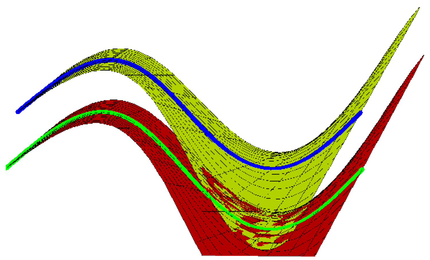
Therefore, for , , , then {, S} is exhibited in Figure 1, where the blue curve demonstrates and the green curve is .
Example 2.
Suppose we are given an admissible curve by
Then,
with and , which shows that is a stationary. For
The surface pencil S over is
Similarly, let in Equation (7), we acquire ,and
Comparably, we have
Ruled Surface Pencil Couple with Bertrand Couple as Joint Principal Curves
Suppose is a ruled surface with the directrix and is also an isoparametric curve of ; then there exists such that . It follows that
where ( explains the orientation of the rulings. In view of Equation (9), we gain
where with . In fact, Equation (22) is a regulation of equations with the three unknowns , and . The resolutions can be deduced as
In view of Equation (15), if is a principal curve on the surface , we get
The above regulations are clearly the necessary and sufficient situations for which is a ruled surface with a directrix ; .
Type I. Non-conoidal or conoidal ruled surfaces for which the wrist (striction) curve does not lie in an Euclidean plane;
Type II. Ruled surfaces for which the wrist curve is in an Euclidean plane;
Type III. Conoidal ruled surfaces for an absolute line as the oriented line in infinity.
We immediately research if the curve is also a principal curve on these three types:
Type I: does not lie in an Euclidean plane and is non-isotropic. Then,
where . From Equations (1), (24), and (26), we have:
which does not satisfy Theorem 2.
Type II: lie in an Euclidean plane and is non-isotropic. Then,
where . From Equations (1), (24), and (28), we gain:
which does not satisfy Theorem 2.
Corollary 2.
In , there are no ruled surface pencil couples of Type I and Type II with Bertrand couples as joint principal curves.
Type III: does not lie in an Euclidean plane and is non-isotropic. Then,
where . From Equations (1), (24), and (29), we have:
where
Equation (31) satisfies Theorem 2. Suppose at all points on , the ruling , , then
for some functions , , and . Replacing it into Equation (25), we get
Then,
Choosing , , and , the ruled surface pencil with can be shown by
Then, the ruled surface pencil is
The functions and can control the shape of the surfaces family and .
Example 3.
Via Example 1, we have:
By taking , then {, } with {,} as joint Bertrand principal curves is (Figure 4):
where the blue curve demonstrates , the green curve is , , and .
By taking , then {, } with {,} as joint Bertrand principal curves is (Figure 5):
where the blue curve demonstrates , the green curve is , , and .
Example 4.
Via Example 2, we have:
(1) By taking , and , then {, } with {,} as joint Bertrand principal curves is (Figure 6):
where the blue curve demonstrates , the green curve is , , and
(2) By taking , and , then {, } with {,} as joint Bertrand principal curves is (Figure 7):
where the blue curve demonstrates , the green curve is , , and
4. Conclusions
This paper studied principal curves and their associated surfaces in Galilean 3-space. Given a 3D curve, we seek surfaces that are faced with this curve as a distinctive curve. The work viewed the Bertrand couples as principal curves and procures a surface pencil couple with a Bertrand couple as joint principal curves. Then, necessary and suffcient conditions for an admissible curve to be an isoparametric principal curve on surface are newly derived in this case. Examples of the surface pencil with principal curves are shown in the figures with a Bertrand couple. Our results in this paper contribute to the work by Jiang et al. [30]. We hope that these outcomes will open modern perceptions for researchers working on geometrical modeling and production evolution procedure in the manufacturing industry. The judgment of stratifying the mechanisms applied here to various spaces such as Lorentz-space, pseudo-Galilean space, and Heisenberg space is already an investigation topic. We will discuss this problem in the future.
Author Contributions
The authors have contributed equally to this work. All authors have read and agreed to the published version of the manuscript.
Funding
This research received no external funding.
Informed Consent Statement
Not applicable.
Data Availability Statement
All of the data are available within the paper.
Conflicts of Interest
The authors declare that there are no conflict of interest regarding the publication of this paper.
References
- Do Carmo, M.P. Differential Geometry of Curves and Surfaces; Prentice Hall: Englewood Cliffs, NJ, USA, 1976. [Google Scholar]
- Spivak, M. A Comprehensive Introduction to Differential Geometry, 2nd ed.; Publish or Perish: Houston, TX, USA, 1979. [Google Scholar]
- Munchmeyer, F.C. On surface imperfections. In Mathematics of Surfaces II; Martin, R., Ed.; Oxford University Press: Oxford, UK, 1987; pp. 459–474. [Google Scholar]
- Patrikalakis, N.M.; Maekawa, T. Shape Interrogation for Computer Aided Design and Manufacturing; Springer: New York, NY, USA, 2002. [Google Scholar]
- Martin, R.R. Principal patches—A new class of surface patches based on differential geometry. In Eurographics 83, Proceedings of the 4th Ann. European Association for Computer Graphics Conference and Exhibition, Zagreb, Yugoslavia, 31 August–2 September 1983; Ten Hagen, P.J.W., Ed.; North-Holland: Amsterdam, The Netherlands, 1983; pp. 47–55. [Google Scholar]
- Alourdas, P.G.; Hottel, G.R.; Tsohy, S.T. A design and interrogation system for modeling with rational splines. In Proceedings of the Ninth International Symposium on OMAE, Houston, TX, USA; AsME: New York, NY, USA, 1990; pp. 555–565. Volume 1, Part B. [Google Scholar]
- Maekawa, T.; Wolter, F.-E.; Patrikalakis, N.M. Umbilics and lines of curvature for shape interrogation. Comput. Aided Geom. Des. 1996, 13, 133–161. [Google Scholar] [CrossRef]
- Che, W.J.; Paul, J.C. Lines of curvature and umbilical points for implicit surfaces. Comput. Aided Geom. Des. 2007, 24, 395–409. [Google Scholar] [CrossRef]
- Zhang, X.P.; Che, W.J.; Paul, J.C. Computing lines of curvature for implicit surfaces. Comput. Geom. Des. 2009, 26, 923–940. [Google Scholar] [CrossRef]
- Kalogerakis, E.; Nowrouzezahrai, D.; Simari, P.; Singh, K. Extracting lines of curvature from noisy point clouds. Comput.-Aided Des. 2009, 41, 282–292. [Google Scholar] [CrossRef]
- Wang, G.; Tang, K.; Tai, C.H. Parametric representation of a surface pencil with common spatial geodesic. Comput.-Aided Des. 2004, 36, 47–59. [Google Scholar] [CrossRef]
- Kauap, E.; Akyldz, F.K.; Orbay, K. A generalization of surfaces family with common spatial geodesic. Appl. Math. Comput. 2008, 201, 781–789. [Google Scholar]
- Li, C.Y.; Wang, R.H.; Zhu, C.G. Parametric representation of a surface pencil with a common line of curvature. Computer Aided Des. 2011, 43, 1110–1117. [Google Scholar] [CrossRef]
- Li, C.Y.; Wang, R.H.; Zhu, C.G. An approach for designing a developable surface through a given line of curvature. Computer Aided Des. 2013, 45, 621–627. [Google Scholar] [CrossRef]
- Bayram, E.; Guler, F.; Kauap, E. Parametric representation of a surface pencil with a common asymptotic curve. Computer Aided Des. 2012, 44, 637–643. [Google Scholar] [CrossRef]
- Liu, Y.; Wang, G.J. Designing developable surface pencil through given curve as its common asymptotic curve. J. Zhejiang Univ. 2013, 47, 1246–1252. [Google Scholar]
- Atalay, G.; Kasap, E. Surfaces family with common smarandache geodesic curve. J. Uci. Artu. 2017, 4, 651–664. [Google Scholar]
- Atalay, G.; Kasap, E. Surfaces family with common smarandache geodesic curve according to Bishop frame in Euclidean space. Math. Sci. 2016, 4, 164–174. [Google Scholar] [CrossRef]
- Bayram, E.; Mustafa, B. Surface family with a common involute asymptotic curve. Int. J. Geom. Methods Mod. Phys. 2016, 13, 447–459. [Google Scholar]
- Guler, F.; Bayram, E.; Kasap, E. Offset surface pencil with a common asymptotic curve. Int. J. Geom. Methods Mod. Phys. 2018, 15, 1850195(1)–1850195(11). [Google Scholar] [CrossRef]
- Atalay, G. Surfaces family with a common Mannheim asymptotic curve. J. Appl. Math. Comput. 2018, 2, 143–154. [Google Scholar]
- Atalay, G. Surfaces family with a common Mannheim geodesic curve. J. Appl. Math. Comput. 2018, 2, 155–165. [Google Scholar]
- Abdel-Baky, R.A.; Alluhaibi, N. Surfaces family with a common geodesic curve in Euclidean 3-upace E3. Inter. J. Math. Anal. 2019, 9, 433–447. [Google Scholar]
- Hobson, M.P.; Efstathiou, G.P.; Lasenby, A.N. General Relativity An Introduction for Physicists; Cambridge University Press: Cambridge, UK, 2006. [Google Scholar]
- Yaglom, I.M. A Simple Non-Euclidean Geometry and Its Physical Basis; Springer: New York, NY, USA, 1979. [Google Scholar]
- Dede, D. Tubular surfaces in Galilean space. Math. Common. 2013, 18, 209–217. [Google Scholar]
- Dede, D.; Ekici, E.; Coken, A.C. On the parallel surfaces in Galilean space. Hacet. J. Math. Stat. 2013, 42, 605–615. [Google Scholar] [CrossRef]
- Yuzbası, Z.K. On a family of surfaces with joint asymptotic curve in the Galilean space . J. Nonlinear Sci. Appl. 2016, 9, 518–523. [Google Scholar] [CrossRef]
- Yuzbası, Z.K.; Bektas, M. On the conutructios of a surface family with joint geodeuic in Galilean space . Open Phys. 2016, 14, 360–363. [Google Scholar] [CrossRef]
- Jiang, X.; Jiang, P.; Meng, J.; Wang, K. Surface pencil couple interpolating Bertrand couple au joint asymptotic curves in Galilean space. Int. J. Geom. Methods Mod. Phys. 2021, 18, 2150114. [Google Scholar] [CrossRef]
- Almoneef, A.A.; Abdel-Baky, R.A. Surface family couple with Bertrand couple au common geodesic curves in Galilean 3-upace . Mathematics 2023, 11, 2391. [Google Scholar]
- Li, Y.; Eren, K.; Ersoy, S. On simultaneous characterizations of partner-ruled surfaces in Minkowski 3-space. AIMS Math. 2023, 8, 22256–22273. [Google Scholar] [CrossRef]
- Li, Y.; Güler, E. A Hypersurfaces of Revolution Family in the Five-Dimensional Pseudo-Euclidean Space . Mathematics 2023, 11, 3427. [Google Scholar]
- Li, Y.; Gupta, M.K.; Sharma, S.; Chaubey, S.K. On Ricci Curvature of a Homogeneous Generalized Matsumoto Finsler Space. Mathematics 2023, 11, 3365. [Google Scholar] [CrossRef]
- Li, Y.; Bhattacharyya, S.; Azami, S.; Saha, A.; Hui, S.K. Harnack Estimation for Nonlinear, Weighted, Heat-Type Equation along Geometric Flow and Applications. Mathematics 2023, 11, 2516. [Google Scholar] [CrossRef]
- Li, Y.; Kumara, H.A.; Siddesha, M.S.; Naik, D.M. Characterization of Ricci Almost Soliton on Lorentzian Manifolds. Symmetry 2023, 15, 1175. [Google Scholar] [CrossRef]
- Li, Y.; Mak, M. Framed Natural Mates of Framed Curves in Euclidean 3-Space. Mathematics 2023, 11, 3571. [Google Scholar]
- Li, Y.; Mofarreh, F.; Abdel-Baky, R.A. Kinematic-geometry of a line trajectory and the invariants of the axodes. Demonstr. Math. 2023, 56, 20220252. [Google Scholar]
- Li, Y.; Patra, D.; Alluhaibi, N.; Mofarreh, F.; Ali, A. Geometric classifications of k-almost Ricci solitons admitting paracontact metrices. Open Math. 2023, 21, 20220610. [Google Scholar] [CrossRef]
- Li, Y.; Güler, E. Hypersurfaces of revolution family supplying in pseudo-Euclidean space. AIMS Math. 2023, 8, 24957–24970. [Google Scholar] [CrossRef]
- Li, Y.; Eren, K.; Ayvacı, K.H.; Ersoy, S. The developable surfaces with pointwise 1-type Gauss map of Frenet type framed base curves in Euclidean 3-space. AIMS Math. 2023, 8, 2226–2239. [Google Scholar] [CrossRef]
- Li, Y.; Ganguly, D. Kenmotsu Metric as Conformal η-Ricci Soliton. Mediterr. J. Math. 2023, 20, 193. [Google Scholar] [CrossRef]
- Li, Y.; Erdoğdu, M.; Yavuz, A. Differential Geometric Approach of Betchow-Da Rios Soliton Equation. Hacet. J. Math. Stat. 2023, 52, 114–125. [Google Scholar] [CrossRef]
- Li, Y.; Abdel-Salam, A.A.; Saad, M.K. Primitivoids of curves in Minkowski plane. AIMS Math. 2023, 8, 2386–2406. [Google Scholar] [CrossRef]
- Li, J.; Yang, Z.; Li, Y.; Abdel-Baky, R.A.; Saad, M.K. On the Curvatures of Timelike Circular Surfaces in Lorentz-Minkowski Space. Filomat 2024, 38, 1–15. [Google Scholar]
- Li, Y.; Gezer, A.; Karakaş, E. Some notes on the tangent bundle with a Ricci quarter-symmetric metric connection. AIMS Math. 2023, 8, 17335–17353. [Google Scholar] [CrossRef]
- Al-Jedani, A.; Abdel-Baky, R.A. A surface family with a mutual geodesic curve in Galilean 3-upace . Mathematics 2023, 11, 2971. [Google Scholar] [CrossRef]
- Roschel, O. Die Geometrie des Galileischen Raumes; Habilitationsschrift: Leoben, Austria, 1984. [Google Scholar]
- Divjak, B. Geometrija Pseudogalilejevih Prostora. Ph.D. Thesis, University of Zagreb, Zagreb, Croatia, 1997. [Google Scholar]
Figure 1.
Curves S (yellow) and (red) with Bertrand couples as joint principal curves.

Figure 2.
Curves S (yellow) and (red) with Bertrand couples as joint principal curves, where .
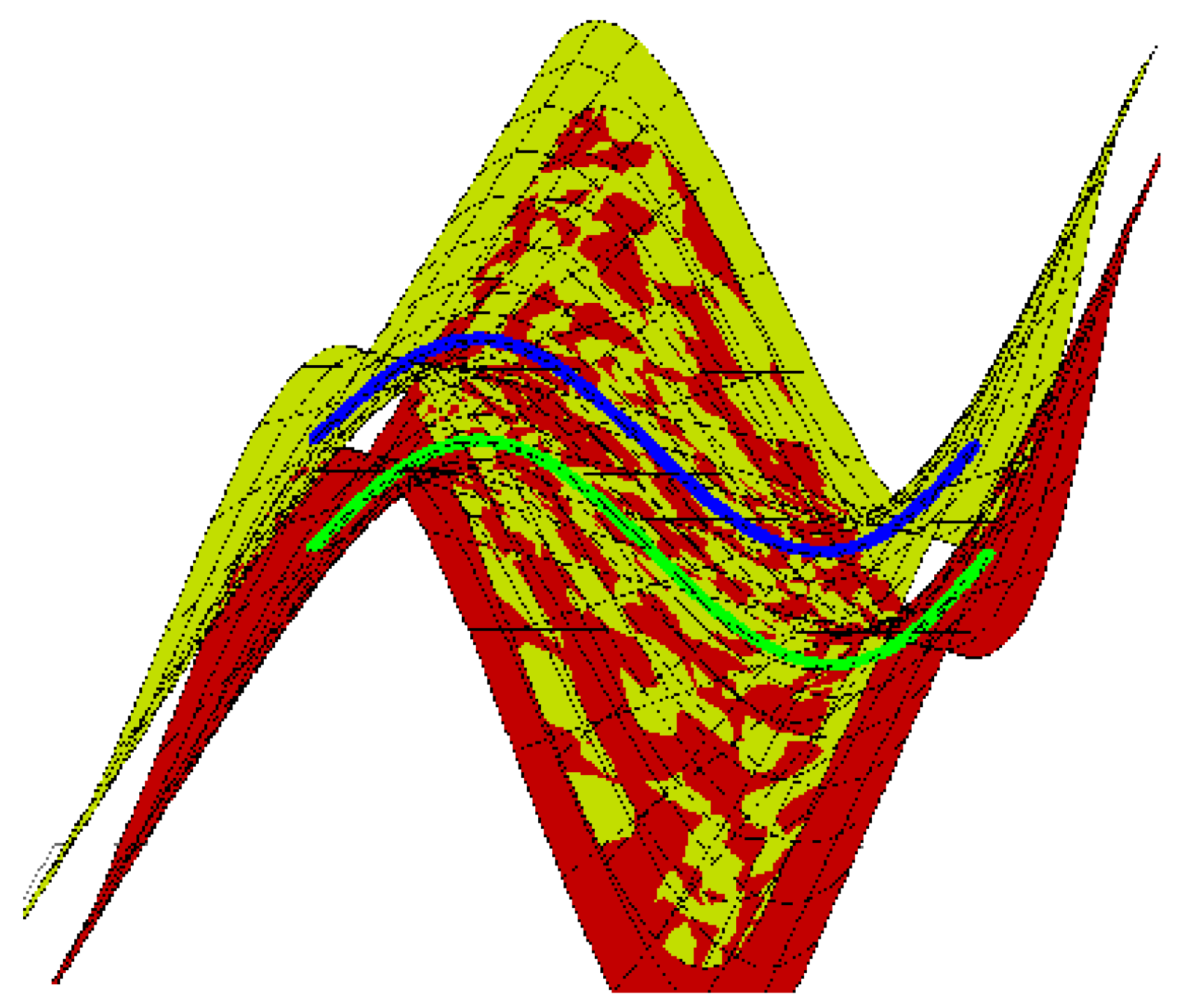
Figure 3.
Curves S (yellow) and (red) with Bertrand couples as joint principal curves, where
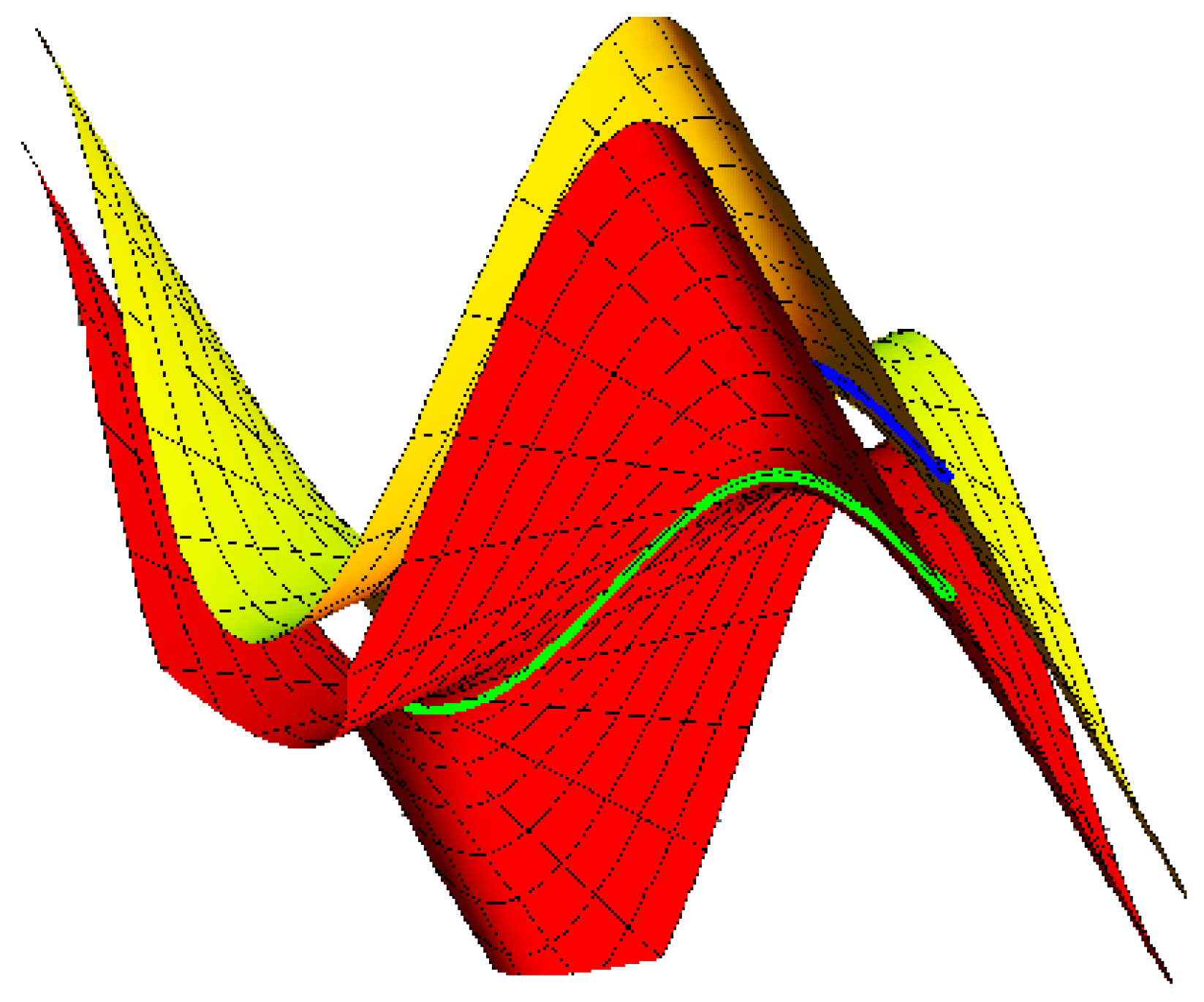
Figure 4.
Curves (yellow) and (red) with Bertrand couples as joint principal curves, where
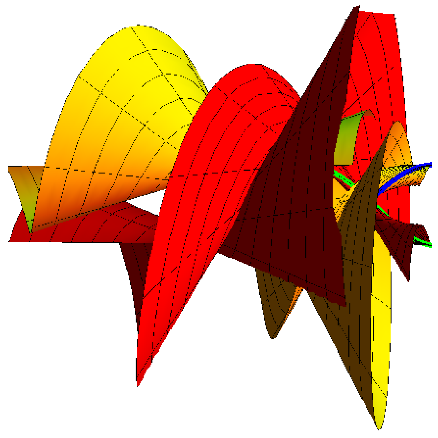
Figure 5.
Surface pencil couple (yellow) and (red).with Bertrand couple as joint principal curves; where
Figure 5.
Surface pencil couple (yellow) and (red).with Bertrand couple as joint principal curves; where
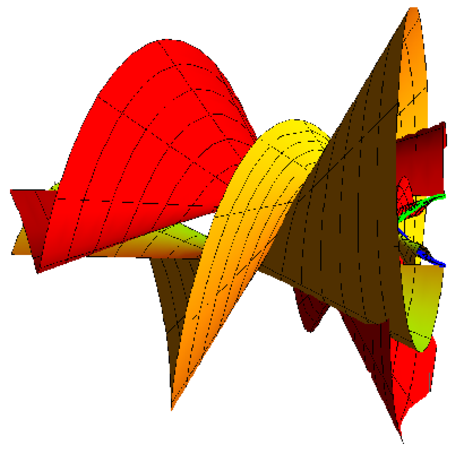
Figure 6.
Curves (yellow) and (red) with Bertrand couples as joint principal curves, where , and

Figure 7.
Curves (yellow) and (red) with Bertrand couples as joint principal curves, where , and
Disclaimer/Publisher’s Note: The statements, opinions and data contained in all publications are solely those of the individual author(s) and contributor(s) and not of MDPI and/or the editor(s). MDPI and/or the editor(s) disclaim responsibility for any injury to people or property resulting from any ideas, methods, instructions or products referred to in the content. |
© 2023 by the authors. Licensee MDPI, Basel, Switzerland. This article is an open access article distributed under the terms and conditions of the Creative Commons Attribution (CC BY) license (https://creativecommons.org/licenses/by/4.0/).
Share and Cite
MDPI and ACS Style
Alluhaibi, N.; Abdel-Baky, R.A. Surface Pencil Couple with Bertrand Couple as Joint Principal Curves in Galilean 3-Space. Axioms 2023, 12, 1022. https://doi.org/10.3390/axioms12111022
AMA Style
Alluhaibi N, Abdel-Baky RA. Surface Pencil Couple with Bertrand Couple as Joint Principal Curves in Galilean 3-Space. Axioms. 2023; 12(11):1022. https://doi.org/10.3390/axioms12111022
Chicago/Turabian StyleAlluhaibi, Nadia, and Rashad A. Abdel-Baky. 2023. "Surface Pencil Couple with Bertrand Couple as Joint Principal Curves in Galilean 3-Space" Axioms 12, no. 11: 1022. https://doi.org/10.3390/axioms12111022
Note that from the first issue of 2016, this journal uses article numbers instead of page numbers. See further details here.