A Study of Monotonicity Analysis for the Delta and Nabla Discrete Fractional Operators of the Liouville–Caputo Family

Abstract

In the present article, we explore the correlation between the sign of a Liouville–Caputo-type difference operator and the monotone behavior of the function upon which the difference operator acts. Finally, an example is also provided to demonstrate the application and the validation of the results which we have proved herein.

1. Introduction

For $s_0\in \mathbb{R}$ we consider the function f from $\{s_0,s_0+1,s_0+2,\cdots \}$ to $\mathbb{R}$. Recall that the nabla (or backward) difference is defined by:

$$(\nabla f)\left(t\right):=f\left(t\right)-f(t-1),t\in \{s_0+1,s_0+2,\cdots \}.$$

It is then easy to show that the following implication holds true:

$$f\mathrm{is}\mathrm{increasing}\mathrm{on}\{s_0,s_0+1,s_0+2,\cdots \}⟺(\nabla f)\left(t\right)\geqq 0\mathrm{for}t\in \{s_0+1,s_0+2,\cdots \}.$$

In fact, an analogous correlation holds true if one considers the delta (or forward) difference, given as follows:

$$\begin{array}{c}\hfill (\Delta f)\left(t\right):=f(t+1)-f\left(t\right),t\in \{s_0,s_0+1,\cdots \}.\end{array}$$

Consequently, in these instances, there exists a clear connection between the sign of the difference and the monotone behavior of the function upon which the difference acts.

Since about 2007, beginning with the foundational work of Atici and Eloe [1,2,3] and continuing with the subsequent work of Abdeljaward, Al-Mdallal and Hajji [4]; Abdeljawad and Atici [5]; Abdeljawad and Baleanu [6]; Abdeljawad and Madjidi [7]; Chen, Bohner and Jia [8]; Ferreira and Torres [9]; Lizama [10]; and Wu and Baleanu [11], there has been increasing interest in a nonlocal version of difference calculus; that is, “discrete fractional calculus". We refer to the recent monograph of Goodrich and Peterson [12] for a wealth of additional information on a variety of nonlocal discrete operators and their properties (see also [13]).

In recent years, discrete fractional operators have gained a lot of attention in numerical computation. Moreover, many researchers have conducted approximations, and numerical methods in particular been suggested and analyzed for the solutions of fractional discrete-time systems; see [14,15].

A particularly curious and mathematically nontrivial aspect of this theory is that there is no clean correlation between the sign of a discrete fractional operator and the monotone (or positive or convex) behavior of the function on which the operator acts. In fact, as has been shown earlier, there is a highly complex and subtle relationship. This mathematically rich behavior was first documented in a monotonicity study by Dahal and Goodrich [16] in 2014. Since their initial study, numerous studies have been published, including those by Atici and Uyanik [17]; Baoguo, Erbe and Peterson [18]; Bravo, Lizama and Rueda [19,20]; Dahal and Goodrich [21]; Du, Jia, Erbe and Peterson [22]; Wang, Jia, Du and Liu [23]; Du and Lu [24]; Goodrich [25]; Baoguo, Erbe and Peterson [26]; Goodrich and Lizama [27]; Baoguo, Erbe and Peterson [28]; Abdeljawad and Abdalla [29]; Chen, Bohner and Jia [30]; Mohammed, Abdeljawad and Hamasalh [31,32]; Liu, Du, Anderson, and Jia [33]; Mohammed, Almutairi, Agarwal and Hamad [34]; and Mohammed, Srivastava, Baleanu, Jan and Abualnaja [35]. These papers investigate a variety of questions surrounding the qualitative properties inferred from the sign of a fractional difference acting on a function.

Above and beyond the pure mathematical interest in this type of problem, there exists a compelling practical reason to care. In the application of both the continuous and the discrete calculus, the ability of the difference (or derivative) to detect when a function is increasing or decreasing is of paramount importance. Thus, clarifying this aspect of the theory of fractional difference operators is important. This is particularly applicable since there have been some initial attempts to apply discrete fractional calculus to biological modeling—see, for example, Atici and Şengül in [36], Atici, Atici, Nguyen, Zhoroev and Koch in [37], and Atici, Atici, Belcher and Marshall in [38].

In this article, we continue to examine these questions within the context of Liouville–Caputo-type fractional differences. The definition of these differences are subtly dissimilar to that of the Riemann–Liouville-type fractional differences, the latter perhaps more commonly studied in discrete cases. Therefore, we believe that there is a good reason to study whether the known results in the Riemann–Liouville case (see, e.g., [16]) carry over to the Liouville-Caputo case. In the case of the nabla Liouville-Caputo difference, the question of monotonicity has already been studied by Baoguo, Erbe and Peterson [18] (see also [12], Chapter 3). However, while their paper addressed the Nabla case, it does not appear to settle the delta case, which, to the best of our knowledge, is still open. In this paper, then, we address this remaining open question. In the process, we also rediscover the nabla results presented in [18] but by a more elementary method—see both Lemma 2 and Theorem 2 later in Section 3. We hope that this investigation will continue to encourage additional investigations of the qualitative data and properties of discrete fractional operators (differences and sums).

2. Preliminaries

Here, we provide some background material regarding fractional sums and differences in delta- and nabla-type operators in the sense of Riemann–Liouville and Liouville–Caputo. These definitions will be important in the work that follows in Section 3.

Definition 1

(see [12,39,40]). Let f be a discrete function on ${\mathbb{N}}_{s_0} :=\{s_0,s_0+1,s_0+2,\dots \}$, $0<\varrho$ be the order of discrete delta and nabla operators, and a be a real number. Then, the delta and nabla fractional sum operators are defined by the following identities:

$$\begin{array}{cc}\hfill \left({{}_{s_0}\Delta }^{-\varrho }f\right)\left(t\right)& :=\sum _{r=s_0}^{t-\varrho }\frac{{\left(t-r-1\right)}^{(\varrho -1)}}{\Gamma \left(\varrho \right)}f\left(r\right),\mathrm{for}t\in {\mathbb{N}}_{s_0+\varrho },\hfill \end{array}$$

and

$$\begin{array}{cc}\hfill \left({{}_{s_0}\nabla }^{-\varrho }f\right)\left(t\right)& :=\sum _{r=s_0+1}^t\frac{{\left(t-r+1\right)}^{[\varrho -1]}}{\Gamma \left(\varrho \right)}f\left(r\right),\mathrm{for}t\in {\mathbb{N}}_{s_0+1},\hfill \end{array}$$

respectively, where $t^{\left(\varrho \right)}$ and $t^{\left[\varrho \right]}$ are defined as follows:

$$\begin{array}{c}\hfill t^{\left(\varrho \right)}:=\mathrm{\Gamma }\left(1+t\right)/\mathrm{\Gamma }\left(1-\varrho +t\right),\mathrm{and}{t}^{\left[\varrho \right]}:=\mathrm{\Gamma }\left(t+\varrho \right)/\mathrm{\Gamma }\left(t\right),\end{array}$$

respectively, for those values of t and ϱ, such that $\mathrm{\Gamma }\left(1+t\right)/\mathrm{\Gamma }\left(1-\varrho +t\right)$ and $\mathrm{\Gamma }\left(t+\varrho \right)/\mathrm{\Gamma }\left(t\right)$ are well defined.

Remark 1.

It is worth recalling that:

• We here use the standard extensions of the domains of $t^{\left(\varrho \right)}$ and $t^{\left[\varrho \right]}$ to define these to be zero when $\mathrm{\Gamma }\left(1+t\right)$ and $\mathrm{\Gamma }\left(t+\varrho \right)$ are well defined, but $\mathrm{\Gamma }\left(1-\varrho +t\right)$ and $\mathrm{\Gamma }\left(t\right)$ are not defined;
• They are both increasing. Further, we have

  $$\begin{array}{c}\hfill \Delta t^{\left(\varrho \right)}=\varrho t^{(\varrho -1)}\mathrm{and}\nabla t^{\left[\varrho \right]}=\varrho t^{[\varrho -1]}.\end{array}$$

  (1)

Definition 2

(see [12,39]; see also [41,42]). The delta and nabla fractional difference operators for the discrete function f in the sense of Liouville–Caputo are given by

$$\begin{array}{cc}\hfill \left({{}_{s_0}{}^{\mathrm{LC}}\Delta }^{\varrho }f\right)\left(t\right)& :=\left({{}_{s_0}\nabla }^{-(\lambda -\varrho )}{\Delta }^{\lambda }f\right)\left(t\right)\hfill \\ \hfill & =\sum _{r=s_0}^{t-\lambda +\varrho }\frac{{\left(t-r-1\right)}^{(\lambda -\varrho -1)}}{\mathrm{\Gamma }(\lambda -\varrho )}\left({\Delta }^{\lambda }f\right)\left(r\right),\mathrm{for}t\mathrm{in}{\mathbb{N}}_{s_0+\lambda -\varrho },\hfill \end{array}$$

(2)

and

$$\begin{array}{cc}\hfill \left({{}_{s_0}{}^{\mathrm{LC}}\nabla }^{\varrho }f\right)\left(t\right)& :=\left({{}_{s_0}\nabla }^{-(\lambda -\varrho )}{\nabla }^{\lambda }f\right)\left(t\right)\hfill \\ \hfill & =\sum _{r=s_0+1}^t\frac{{\left(t-r+1\right)}^{[\lambda -\varrho -1]}}{\mathrm{\Gamma }(\lambda -\varrho )}\left({\nabla }^{\lambda }f\right)\left(r\right),\mathrm{for}t\mathrm{in}{\mathbb{N}}_{s_0+\lambda },\hfill \end{array}$$

(3)

respectively, where $\lambda \in {\mathbb{N}}_{s_0+1}$ satisfies the inequality $\lambda -1<\varrho <\lambda$.

3. Delta and Nabla Monotonicity Results

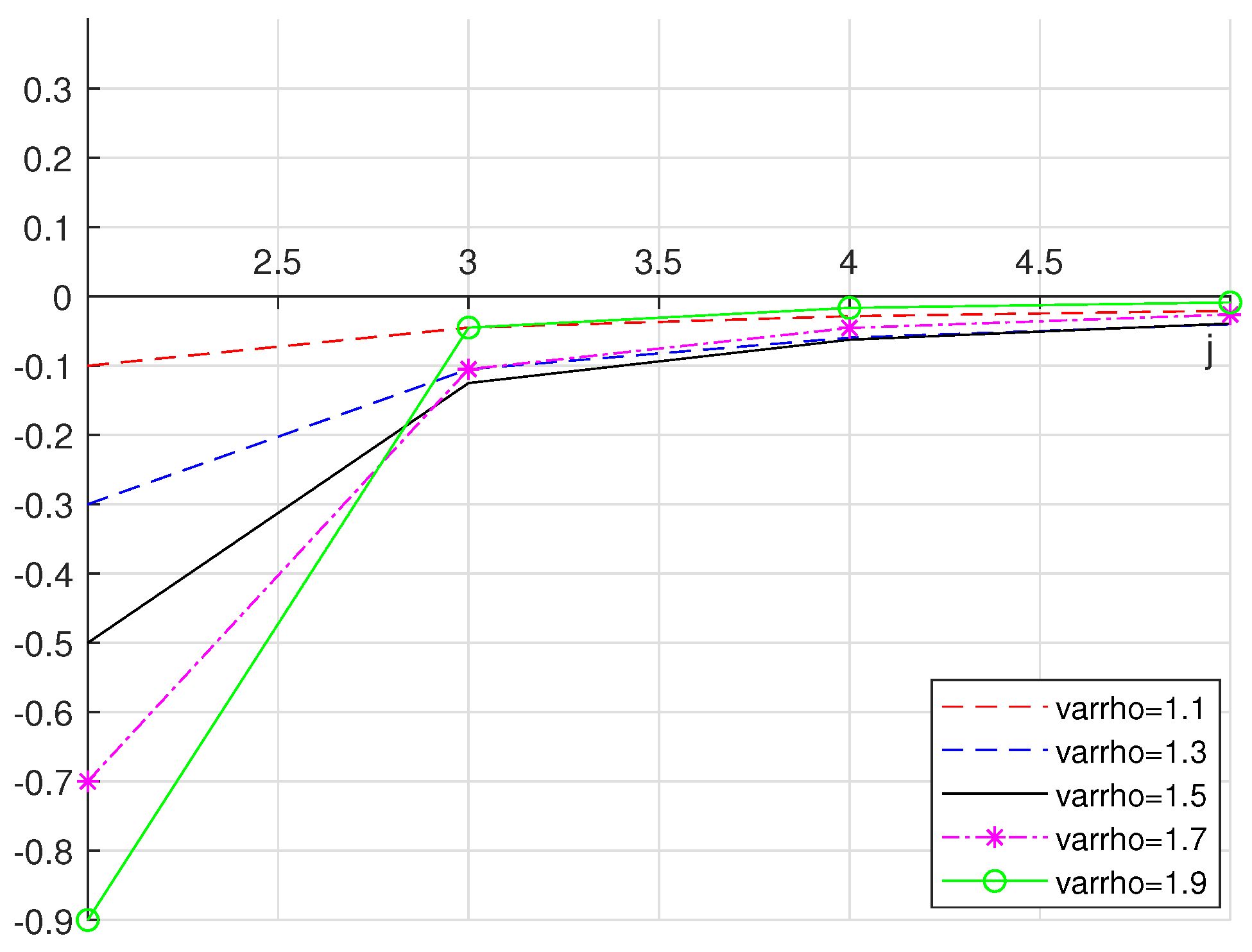
The following are the main lemmas when the order $\varrho$ of the difference operators are in the interval $1<\varrho <2$. The first lemma concerns the fractional delta difference.

Lemma 1.

For a discrete function f on ${\mathbb{N}}_{s_0},$ the delta Liouville–Caputo difference operator can be rewritten in the following form:

$$\begin{array}{c}\left({{}_{s_0}{}^{\mathrm{LC}}\Delta }^{\varrho }f\right)(s_0+k+2-\varrho )=\left(\Delta f\right)(s_0+k+1)\hfill \\ \hfill -\frac{{\left(k+1-\varrho \right)}^{(1-\varrho )}}{\mathrm{\Gamma }(2-\varrho )}(\Delta f)\left(s_0\right)+\sum _{r=s_0+1}^{s_0+k}\frac{{\left(s_0+k+1-\varrho -r\right)}^{(-\varrho )}}{\mathrm{\Gamma }(1-\varrho )}\left(\Delta f\right)\left(r\right)(k\in {\mathbb{N}}_0),\end{array}$$

(4)

where

$$\begin{array}{c}\hfill \frac{{\left(s_0+k+1-\varrho -r\right)}^{(-\varrho )}}{\mathrm{\Gamma }(1-\varrho )}<0,\end{array}$$

(5)

for $k\in {\mathbb{N}}_1$.

Proof. 

We consider Definition (2) for $\lambda =2$ (that is, $1<\varrho <2$). For $t\in {\mathbb{N}}_{s_0+2-\varrho }$, we thus obtain

$$\begin{array}{cc}\hfill \left({{}_{s_0}{}^{\mathrm{LC}}\Delta }^{\varrho }f\right)\left(t\right)& =\sum _{r=s_0}^{t+\varrho -2}\frac{{\left(t-r-1\right)}^{(1-\varrho )}}{\mathrm{\Gamma }(2-\varrho )}\left({\Delta }^{2}f\right)\left(r\right)\hfill \\ \hfill & =\sum _{r=s_0}^{t+\varrho -2}\frac{{\left(t-r-1\right)}^{(1-\varrho )}}{\mathrm{\Gamma }(2-\varrho )}\left(\Delta f\right)(r+1)-\sum _{r=s_0}^{t+\varrho -2}\frac{{\left(t-r-1\right)}^{(1-\varrho )}}{\mathrm{\Gamma }(2-\varrho )}\left(\Delta f\right)\left(r\right)\hfill \\ \hfill & =-\frac{{(t-s_0-1)}^{(1-\varrho )}}{\mathrm{\Gamma }(2-\varrho )}\left(\Delta f\right)\left(s_0\right)+\sum _{r=s_0+1}^{t+\varrho -1}\frac{{\left(t-r\right)}^{(1-\varrho )}}{\mathrm{\Gamma }(2-\varrho )}\left(\Delta f\right)\left(r\right)\hfill \\ \hfill & -\sum _{r=s_0+1}^{t+\varrho -1}\frac{{\left(t-r-1\right)}^{(1-\varrho )}}{\mathrm{\Gamma }(2-\varrho )}\left(\Delta f\right)\left(r\right)\hfill \\ \hfill & =-\frac{{(t-s_0-1)}^{(1-\varrho )}}{\mathrm{\Gamma }(2-\varrho )}\left(\Delta f\right)\left(s_0\right)+\sum _{r=s_0+1}^{t+\varrho -1}\frac{{\Delta }_t{\left(t-r-1\right)}^{(1-\varrho )}}{\mathrm{\Gamma }(2-\varrho )}(\Delta f)\left(r\right)\hfill \\ \hfill & \stackrel{by}{\underset{\left(1\right)}{=}}\left(\Delta f\right)\left(t+\varrho -1\right)-\frac{{(t-s_0-1)}^{(1-\varrho )}}{\mathrm{\Gamma }(2-\varrho )}\left(\Delta f\right)\left(s_0\right)+\sum _{r=s_0+1}^{t+\varrho -2}\frac{{\left(t-r-1\right)}^{(-\varrho )}}{\mathrm{\Gamma }(1-\varrho )}(\Delta f)\left(r\right),\hfill \end{array}$$

where we have used the fact that ${(-\varrho )}^{(1-\varrho )}:=0$. By changing the variable $t:=s_0+k+2-\varrho$ for $k\in {\mathbb{N}}_0$, we obtain (4) as desired.

For the second part: for $r=s_0+1,s_0+2,\dots ,s_0+k$ with $k\in {\mathbb{N}}_1$, we have

$$\begin{array}{cc}\hfill \frac{{\left(s_0+k+1-\varrho -r\right)}^{(-\varrho )}}{\mathrm{\Gamma }(1-\varrho )}& =\frac{\mathrm{\Gamma }\left(s_0+k+2-\varrho -r\right)}{\mathrm{\Gamma }(1-\varrho )\mathrm{\Gamma }(s_0+k+2-r)}\hfill \\ \hfill & =\frac{\mathrm{\Gamma }\left(-\varrho +j+1\right)}{\mathrm{\Gamma }(1-\varrho )\mathrm{\Gamma }(j+1)}\left[\mathrm{denoting}j:=s_0+k+1-r=1,2,\dots ,k\right]\hfill \\ \hfill & =\frac{(-\varrho +j)(-\varrho +j-1)\cdots (-\varrho +2)(-\varrho +1)}{j!},\hfill \end{array}$$

which is negative for $\varrho \in (1,2)$. Hence, the proof of (5) is complete. Consequently, Lemma 1 is proved. □

Our second lemma concerns the fractional nabla difference.

Lemma 2.

For a discrete function f on ${\mathbb{N}}_{s_0},$ the nabla Liouville–Caputo difference operator can be rewritten in the following form:

$$\begin{array}{c}\left({{}_{s_0+1}{}^{\mathrm{LC}}\nabla }^{\varrho }f\right)\left(t\right)=\left(\nabla f\right)\left(t\right)-\frac{{\left(t-s_0-1\right)}^{[1-\varrho ]}}{\mathrm{\Gamma }(2-\varrho )}\left(\nabla f\right)(s_0+1)\hfill \\ +\sum _{r=s_0+2}^{t-1}\frac{{\left(t-r+1\right)}^{[-\varrho ]}}{\mathrm{\Gamma }(1-\varrho )}\left(\nabla f\right)\left(r\right)(t\in {\mathbb{N}}_{s_0+2}),\hfill \end{array}$$

(6)

where

$$\begin{array}{c}\hfill \frac{{\left(t-r+1\right)}^{[-\varrho ]}}{\mathrm{\Gamma }(1-\varrho )}<0.\end{array}$$

(7)

Proof. 

According to Definition (3) with $\lambda =2$, for $t\in {\mathbb{N}}_{s_0+2}$ we have

$$\begin{array}{cc}\hfill \left({{}_{s_0+1}{}^{\mathrm{LC}}\nabla }^{\varrho }f\right)\left(t\right)& =\sum _{r=s_0+2}^t\frac{{\left(t-r+1\right)}^{[1-\varrho ]}}{\mathrm{\Gamma }(2-\varrho )}\left({\nabla }^{2}f\right)\left(r\right)\hfill \\ \hfill & =\sum _{r=s_0+2}^t\frac{{\left(t-r+1\right)}^{[1-\varrho ]}}{\mathrm{\Gamma }(2-\varrho )}\left(\nabla f\right)\left(r\right)-\sum _{r=s_0+2}^t\frac{{\left(t-r+1\right)}^{[1-\varrho ]}}{\mathrm{\Gamma }(2-\varrho )}\left(\nabla f\right)(r-1)\hfill \\ \hfill & =-\frac{{(t-s_0-1)}^{(1-\varrho )}}{\mathrm{\Gamma }(2-\varrho )}\left(\nabla f\right)(s_0+1)+\sum _{r=s_0+2}^t\frac{{\left(t-r+1\right)}^{[1-\varrho ]}}{\mathrm{\Gamma }(2-\varrho )}\left(\nabla f\right)\left(r\right)\hfill \\ \hfill & -\sum _{r=s_0+2}^t\frac{{\left(t-r\right)}^{[1-\varrho ]}}{\mathrm{\Gamma }(2-\varrho )}\left(\nabla f\right)\left(r\right)\hfill \\ \hfill & =-\frac{{(t-s_0-1)}^{[1-\varrho ]}}{\mathrm{\Gamma }(2-\varrho )}\left(\nabla f\right)(s_0+1)+\sum _{r=s_0+2}^t\frac{{\nabla }_t{\left(t-r+1\right)}^{[1-\varrho ]}}{\mathrm{\Gamma }(2-\varrho )}(\nabla f)\left(r\right)\hfill \\ \hfill & \stackrel{by}{\underset{\left(1\right)}{=}}\left(\nabla f\right)\left(t\right)-\frac{{(t-s_0-1)}^{[1-\varrho ]}}{\mathrm{\Gamma }(2-\varrho )}\left(\nabla f\right)(s_0+1)+\sum _{r=s_0+2}^{t-1}\frac{{\left(t-r+1\right)}^{[-\varrho ]}}{\mathrm{\Gamma }(1-\varrho )}(\nabla f)\left(r\right),\hfill \end{array}$$

where we have used the fact that ${\left(0\right)}^{[1-\varrho ]}:=0$. This completes the proof of (6).

For the second part, we let $j:=t-r=1,2,\dots$ when $r=s_0+2,s_0+3,\dots ,t-1$ with $t\in {\mathbb{N}}_{s_0+3}$. Then, using the same technique for (7), we can achieve the proof of (7). Therefore, the proof of Lemma 2 is complete. □

Remark 2.

It is of interest to mention that the expressions (5) in Lemma 1 and (7) in Lemma 2 are the same; this is easy to check by writing out the relevant expressions. Here, we illustrate it graphically in Figure 1 below for different values of ϱ in the interval $(1,2)$.

Based on the above lemmas, we now can state and prove our monotonicity theorems. The first such result, Theorem 1, concerns the delta case and, as such, complements the results of Baoguo, Erbe and Peterson [18], as already mentioned in Section 1.

Theorem 1.

Let $\varrho \in (1,2)$. Suppose that f is defined on ${\mathbb{N}}_{s_0}$ such that

$$\begin{array}{cc}\hfill & \left({{}_{s_0}{}^{\mathrm{LC}}\Delta }^{\varrho }f\right)\left(t\right)\geqq 0,t\in {\mathbb{N}}_{s_0+2-\varrho },\hfill \\ \hfill & f(s_0+1)\geqq f\left(s_0\right)\geqq 0.\hfill \end{array}$$

Then $f\left(t\right)$ is monotonically increasing, that is,

$$\left(\Delta f\right)\left(t\right)\geqq 0\mathrm{for}t\in {\mathbb{N}}_{s_0}.$$

Proof. 

The proof can be done according to the principle of strong mathematical induction on k. Considering the assumption in the statement of the theorem that $f(s_0+1)\geqq f\left(s_0\right)$, we find that $\left(\Delta f\right)\left(s_0\right)\geqq 0$. Suppose, for the induction hypothesis, that

$$\left(\Delta f\right)(s_0+j)\geqq 0,$$

where $j=0,1,2,\dots ,k$ for some $k\in {\mathbb{N}}_0$. Then, by using $\left({{}_{s_0}{}^{\mathrm{LC}}\Delta }^{\varrho }f\right)\left(t\right)\geqq 0$ in Lemma 1, we find

$$\begin{array}{cc}\hfill \left(\Delta f\right)(s_0+1+k)& \geqq \frac{{\left(k+1-\varrho \right)}^{(1-\varrho )}}{\mathrm{\Gamma }(2-\varrho )}(\Delta f)\left(s_0\right)\hfill \\ \hfill & -\sum _{r=s_0+1}^{s_0+k}\underset{<0\mathrm{by}\left(5\right)}{\underbrace{\frac{{\left(s_0+k+1-\varrho -r\right)}^{(-\varrho )}}{\mathrm{\Gamma }(1-\varrho )}}}\underset{\geqq 0\mathrm{by}\mathrm{induction}\mathrm{hypothesis}}{\underbrace{\left(\Delta f\right)\left(r\right)}}\hfill \\ \hfill & \geqq \frac{{\left(k+1-\varrho \right)}^{(1-\varrho )}}{\mathrm{\Gamma }(2-\varrho )}\underset{\geqq 0\mathrm{by}\mathrm{assumption}}{\underbrace{(\Delta f)\left(s_0\right)}}\hfill \\ \hfill & \geqq 0.\hfill \end{array}$$

Moreover, since for $1<\varrho <2$, we see that

$$\begin{array}{cc}\hfill \frac{{\left(k+1-\varrho \right)}^{(1-\varrho )}}{\mathrm{\Gamma }(2-\varrho )}& =\frac{\mathrm{\Gamma }(k+2-\varrho )}{\mathrm{\Gamma }(2-\varrho )\mathrm{\Gamma }(k+1)}\hfill \\ \hfill & =\left\{\begin{array}{cc}\frac{1}{0!}>0,\hfill & \mathrm{for}k=0,\hfill \\ \frac{(-\varrho +2)}{1!}>0,\hfill & \mathrm{for}k=1,\hfill \\ \frac{(-\varrho +2)(-\varrho +3)\cdots (-\varrho +k)(-\varrho +k+1)}{k!}>0,\hfill & \mathrm{for}k\geqq 2.\hfill \end{array}\right.\hfill \end{array}$$

(8)

Thus, clearly, $\left(\Delta f\right)(s_0+k+1)\geqq 0$. Hence, $\left(\Delta f\right)\left(t\right)\geqq 0$, as asserted for $t\in {\mathbb{N}}_{s_0}$. □

Our second monotonicity result (namely, Theorem 2 below) provides an alternative proof of one of the results in Baoguo, Erbe and Peterson [18].

Theorem 2.

Let $\varrho \in (1,2)$. Suppose that f is defined on ${\mathbb{N}}_{s_0}$ such that

$$\begin{array}{cc}\hfill & \left({{}_{s_0+1}{}^{\mathrm{LC}}\nabla }^{\varrho }f\right)\left(t\right)\geqq 0,t\in {\mathbb{N}}_{s_0+2},\hfill \\ \hfill & f(s_0+1)\geqq f\left(s_0\right)\geqq 0.\hfill \end{array}$$

Then $f\left(t\right)$ is monotonically increasing, that is,

$$\left(\nabla f\right)\left(t\right)\geqq 0\mathrm{for}t\in {\mathbb{N}}_{s_0+1}.$$

Proof. 

Again, we prove the desired result by using the principle of strong mathematical induction on k. By the assumptions given in the statement of the theorem, we see that $\left(\nabla f\right)(s_0+1)\geqq 0$. Moreover, we know from Lemma 2 that

$$\begin{array}{cc}\hfill \left(\nabla f\right)(s_0+2)& \geqq \frac{{\left(1\right)}^{[1-\varrho ]}}{\mathrm{\Gamma }(2-\varrho )}\left(\nabla f\right)(s_0+1)-\underset{=0}{\underbrace{\sum _{r=s_0+2}^{s_0+1}\frac{{\left(s_0+3-r\right)}^{[-\varrho ]}}{\mathrm{\Gamma }(1-\varrho )}\left(\nabla f\right)\left(r\right)}}\hfill \\ \hfill & =\left(\nabla f\right)(s_0+1)\geqq 0.\hfill \end{array}$$

We now assume that $\left(\nabla f\right)(s_0+j)\geqq 0$, where $j=1,2,\dots ,k$ for some $k\in {\mathbb{N}}_1$. Then, by using the assumption that $\left({{}_{s_0+1}{}^{\mathrm{LC}}\nabla }^{\varrho }f\right)\left(t\right)\geqq 0$ into Lemma 2, we can deduce that

$$\begin{array}{cc}\hfill \left(\nabla f\right)(s_0+1+k)& \geqq \frac{{\left(k\right)}^{[1-\varrho ]}}{\mathrm{\Gamma }(2-\varrho )}(\nabla f)(s_0+1)-\sum _{r=s_0+2}^{s_0+k}\underset{<0\mathrm{by}\left(7\right)}{\underbrace{\frac{{\left(s_0+k+2-r\right)}^{[-\varrho ]}}{\mathrm{\Gamma }(1-\varrho )}}}\underset{\geqq 0\mathrm{by}\mathrm{induction}\mathrm{hypothesis}}{\underbrace{\left(\nabla f\right)\left(r\right)}}\hfill \\ \hfill & \geqq \frac{{\left(k\right)}^{[1-\varrho ]}}{\mathrm{\Gamma }(2-\varrho )}\underset{\geqq 0\mathrm{by}\mathrm{assumption}}{\underbrace{(\nabla f)(s_0+1)}}\hfill \\ \hfill & \geqq 0,\hfill \end{array}$$

where the following results were used:

$$\begin{array}{cc}\hfill \frac{{\left(k\right)}^{(1-\varrho )}}{\mathrm{\Gamma }(2-\varrho )}& =\frac{\mathrm{\Gamma }(1+k-\varrho )}{\mathrm{\Gamma }(2-\varrho )\mathrm{\Gamma }\left(k\right)}\hfill \\ \hfill & =\frac{\mathrm{\Gamma }(k_1+2-\varrho )}{\mathrm{\Gamma }(2-\varrho )\mathrm{\Gamma }(k_1+1)}>0\left[\mathrm{denoting}{k}_1:=k-1\geqq 0\right],\hfill \end{array}$$

as we have proved in (8). Therefore,

$$\left(\nabla f\right)(s_0+k+1)\geqq 0.$$

Hence, $\left(\nabla f\right)\left(t\right)\geqq 0$ as asserted for $t\in {\mathbb{N}}_{s_0+1}$. □

4. Example

In our final section, we provide a specific example to illustrate the results of Section 3.

Example 1.

Consider the function f given by

$$\begin{array}{c}\hfill f\left(t\right)={\left(\frac{3}{2}\right)}^t,\mathrm{for}t\in {\mathbb{N}}_{s_0+2}.\end{array}$$

At first, we will try to show that

$$\left({{}_{s_0}{}^{\mathrm{LC}}\Delta }^{\varrho }f\right)\left(t\right)\geqq 0\mathrm{for}t\in \{s_0+2-\varrho ,s_0+3-\varrho \},\varrho =\frac{3}{2}\mathrm{and}{s}_0=0.$$

We see from (4) at $k=0$ that

$$\begin{array}{cc}\hfill \left({{}_{s_0}{}^{\mathrm{LC}}\Delta }^{\varrho }f\right)(s_0+2-\varrho )& =\left(\Delta f\right)(s_0+1)-\frac{{(1-\varrho )}^{(1-\varrho )}}{\mathrm{\Gamma }(2-\varrho )}\left(\Delta f\right)\left(s_0\right)\hfill \\ \hfill & +\underset{=0}{\underbrace{\sum _{r=s_0+1}^{s_0}\frac{{(s_0+1-\varrho -r)}^{(-\varrho )}}{\mathrm{\Gamma }(1-\varrho )}f\left(r\right)}}\hfill \\ \hfill & =-\left(\Delta f\right)\left(s_0\right)+\left(\Delta f\right)(s_0+1)\hfill \\ \hfill & =f(s_0+2)-2f(s_0+1)+f\left(s_0\right)=\frac{1}{4}\geqq 0,\hfill \end{array}$$

which yields

$$\begin{array}{c}\hfill \left(\Delta f\right)(s_0+1)\geqq \left(\Delta f\right)\left(s_0\right)\geqq 0.\end{array}$$

(9)

Additionally, in the case when $k=1$, we find from (4) that

$$\begin{array}{cc}\hfill & \left({{}_{s_0}{}^{\mathrm{LC}}\Delta }^{\varrho }f\right)(s_0+3-\varrho )\hfill \\ \hfill & =\left(\Delta f\right)(s_0+2)-\frac{{(2-\varrho )}^{(1-\varrho )}}{\mathrm{\Gamma }(2-\varrho )}\left(\Delta f\right)\left(s_0\right)+\sum _{r=s_0+1}^{s_0+2}\frac{{(s_0+2-\varrho -r)}^{(-\varrho )}}{\mathrm{\Gamma }(1-\varrho )}f\left(r\right)\hfill \\ \hfill & =-(2-\varrho )\left(\Delta f\right)\left(s_0\right)+(1-\varrho )\left(\Delta f\right)(s_0+1)+\left(\Delta f\right)(s_0+2)\hfill \\ \hfill & =-\frac{1}{2}\left(f\left(1\right)-f\left(0\right)\right)-\frac{1}{2}\left(f\left(2\right)-f\left(1\right)\right)+f\left(3\right)-f\left(2\right)=\frac{1}{2}\geqq 0.\hfill \end{array}$$

This, together with (9), implies that

$$\begin{array}{c}\hfill \left(\Delta f\right)(s_0+2)\geqq (\varrho -1)\left(\Delta f\right)(s_0+1)+(2-\varrho )\left(\Delta f\right)\left(s_0\right)\geqq 0.\end{array}$$

On the other hand, from (6) we have

$$\begin{array}{cc}\hfill \left({{}_{s_0+1}{}^{\mathrm{LC}}\nabla }^{\varrho }f\right)(s_0+2)& =\left(\nabla f\right)(s_0+2)-\frac{{\left(1\right)}^{[1-\varrho ]}}{\mathrm{\Gamma }(2-\varrho )}\left(\nabla f\right)(s_0+1)\hfill \\ \hfill & +\underset{=0}{\underbrace{\sum _{r=s_0+2}^{s_0+1}\frac{{(s_0+3-r)}^{[-\varrho ]}}{\mathrm{\Gamma }(1-\varrho )}f\left(r\right)}}\hfill \\ \hfill & =\left(\nabla f\right)(s_0+2)-\left(\nabla f\right)(s_0+1)\hfill \\ \hfill & =f(s_0+2)-2f(s_0+1)+f\left(s_0\right)=\frac{1}{4}\geqq 0,\hfill \end{array}$$

which yields

$$\begin{array}{c}\hfill \left(\nabla f\right)(s_0+2)\geqq \left(\nabla f\right)(s_0+1)\geqq 0.\end{array}$$

Consequently, we see that f is nondecreasing on $\{s_0+1,s_0+2,s_0+3\}$.

5. Conclusions and Future Directions

In this paper, we have provided further analysis of the relationship between the sign of the monotonicity of a function f and $\left({{}_{s_0}{}^{\mathrm{LC}}\Delta }^{\varrho }f\right)\left(t\right)$ and $\left({{}_{s_0+1}{}^{\mathrm{LC}}\nabla }^{\varrho }f\right)\left(t\right)$ acting on f. We filled an apparent gap in the literature regarding the delta Liouville–Caputo type difference, and we have also presented a different and presumably simpler proof of a result that can be found in an earlier paper by Baoguo et al. [18]. We continue to see that the qualitative behaviors of discrete fractional operators possess a mathematical richness that their local counterparts do not.

References

1. Atici, F.M.; Eloe, P.W. A transform method in discrete fractional calculus. Int. J. Differ. Equ. 2007, 2, 165–176. [Google Scholar]
2. Atici, F.M.; Eloe, P.W. Discrete fractional calculus with the nabla operator. Electron. J. Qual. Theory Differ. Equ. 2009, 2009, 1–12. [Google Scholar] [CrossRef]
3. Atici, F.M.; Eloe, P.W. Initial value problems in discrete fractional calculus. Proc. Am. Math. Soc. 2009, 137, 981–989. [Google Scholar] [CrossRef]
4. Abdeljawad, T.; Al-Mdallal, Q.M.; Hajji, M.A. Arbitrary order fractional difference operators with discrete exponential kernels and applications. Discrete Dyn. Nat. Soc. 2017, 2017, 4149320. [Google Scholar] [CrossRef] [Green Version]
5. Abdeljawad, T.; Atici, F. On the definitions of nabla fractional operators. Abstr. Appl. Anal. 2012, 2012, 406757. [Google Scholar] [CrossRef] [Green Version]
6. Abdeljawad, T.; Baleanu, D. Monotonicity analysis of a nabla discrete fractional operator with discrete Mittag-Leffler kernel. Chaos Solitons Fractals 2017, 102, 106–110. [Google Scholar] [CrossRef]
7. Abdeljawad, T.; Madjidi, F. Lyapunov-type inequalities for fractional difference operators with discrete Mittag-Leffler kernel of order 2 < α < 5/2. Eur. Phys. J. Spec. Top. 2017, 226, 3355–3368. [Google Scholar]
8. Chen, C.R.; Bohner, M.; Jia, B.G. Ulam-Hyers stability of Caputo fractional difference equations. Math. Methods Appl. Sci. 2019, 42, 7461–7470. [Google Scholar] [CrossRef]
9. Ferreira, R.A.C.; Torres, D.F.M. Fractional h-difference equations arising from the calculus of variations. Appl. Anal. Discret. Math. 2011, 5, 110–121. [Google Scholar] [CrossRef] [Green Version]
10. Lizama, C. The Poisson distribution, abstract fractional difference equations, and stability. Proc. Am. Math. Soc. 2017, 145, 3809–3827. [Google Scholar] [CrossRef]
11. Wu, G.; Baleanu, D. Discrete chaos in fractional delayed logistic maps. Nonlinear Dyn. 2015, 80, 1697–1703. [Google Scholar] [CrossRef]
12. Goodrich, C.S.; Peterson, A.C. Discrete Fractional Calculus; Springer: Berlin, Germany, 2015. [Google Scholar]
13. Kilbas, A.A.; Srivastava, H.M.; Trujillo, J.J. Theory and Applications of Fractional Differential Equations; North-Holland Mathematics Studies; Elsevier: Amsterdam, The Netherlands, 2006; Volume 204. [Google Scholar]
14. Wu, G.C.; Song, T.T.; Wang, S.Q. Caputo-Hadamard fractional differential equation on time scales: Numerical scheme, asymptotic stability, and chaos. Chaos 2022, 32, 093143. [Google Scholar] [CrossRef]
15. Song, T.T.; Wu, G.C.; Wei, J.L. Hadamard fractional calculus on time scales. Fractals 2022, 30, 2250145. [Google Scholar] [CrossRef]
16. Dahal, R.; Goodrich, C.S. A monotonicity result for discrete fractional difference operators. Arch. Math. 2014, 102, 293–299. [Google Scholar] [CrossRef]
17. Atici, F.; Uyanik, M. Analysis of discrete fractional operators. Appl. Anal. Discrete Math. 2015, 9, 139–149. [Google Scholar] [CrossRef]
18. Baoguo, J.; Erbe, L.; Peterson, A. Some relations between the Caputo fractional difference operators and integer-order differences. Electron. J. Differ. Equ. 2015, 2015, 1–7. [Google Scholar]
19. Bravo, J.; Lizama, C.; Rueda, S. Second and third order forward difference operator: What is in between? Rev. R. Acad. Cienc. Exactas Fis. Nat. Ser. A Mat. RACSAM 2021, 115, 86. [Google Scholar] [CrossRef]
20. Bravo, J.; Lizama, C.; Rueda, S. Qualitative properties of nonlocal discrete operators. Math. Methods Appl. Sci. 2022, 45, 6346–6377. [Google Scholar] [CrossRef]
21. Dahal, R.; Goodrich, C.S. Mixed order monotonicity results for sequential fractional nabla differences. J. Differ. Equ. Appl. 2019, 25, 837–854. [Google Scholar] [CrossRef]
22. Du, F.; Jia, B.; Erbe, L.; Peterson, A. Monotonicity and convexity for nabla fractional (q, h)-differences. J. Differ. Equ. Appl. 2016, 22, 1224–1243. [Google Scholar] [CrossRef]
23. Wang, M.; Jia, B.G.; Du, F.F.; Liu, X. Asymptotic stability of fractional difference equations with bounded time delays. Fract. Calc. Appl. Anal. 2020, 23, 571–590. [Google Scholar] [CrossRef]
24. Du, F.F.; Lu, J.G. Finite-time stability of neutral fractional order time delay systems with Lipschitz nonlinearities. Appl. Math. Comput. 2020, 375, 125079. [Google Scholar] [CrossRef]
25. Goodrich, C.S. A sharp convexity result for sequential fractional delta differences. J. Differ. Equ. Appl. 2017, 23, 1986–2003. [Google Scholar] [CrossRef]
26. Baoguo, J.; Erbe, L.; Peterson, A. Convexity for nabla and delta fractional differences. J. Differ. Equ. Appl. 2015, 21, 360–373. [Google Scholar] [CrossRef]
27. Goodrich, C.S.; Lizama, C. Positivity, monotonicity, and convexity for convolution operators. Discret. Contin. Dyn. Syst. 2020, 40, 4961–4983. [Google Scholar] [CrossRef]
28. Baoguo, J.; Erbe, L.; Peterson, A. Monotonicity and convexity for nabla fractional q-differences. Dynam. Syst. Appl. 2016, 25, 47–60. [Google Scholar]
29. Abdeljawad, T.; Abdalla, B. Monotonicity results for delta and nabla Caputo and Riemann fractional differences via dual identities. Filomat 2017, 31, 3671–3683. [Google Scholar] [CrossRef]
30. Chen, C.R.; Bohner, M.; Jia, B.G. Methods of upper and lower solutions for nonlinear Caputo fractional difference equations and its applications. Frac. Calc. Appl. Anal. 2019, 22, 1307–1320. [Google Scholar] [CrossRef]
31. Mohammed, P.O.; Abdeljawad, T.; Hamasalh, F.K. On discrete delta Caputo-Fabrizio fractional operators and monotonicity analysis. Fractal Fract. 2021, 5, 116. [Google Scholar] [CrossRef]
32. Mohammed, P.O.; Srivastava, H.M.; Baleanu, D.; Elattar, E.E.; Hamed, Y.S. Positivity analysis for the discrete delta fractional differences of the Riemann-Liouville and Liouville-Caputo types. Electron. Res. Arch. 2022, 30, 3058–3070. [Google Scholar] [CrossRef]
33. Liu, X.; Du, F.; Anderson, D.; Jia, B. Monotonicity results for nabla fractional h-difference operators. Math. Methods Appl. Sci. 2020, 44, 1207–1218. [Google Scholar] [CrossRef]
34. Mohammed, P.O.; Almutairi, O.; Agarwal, R.P.; Hamed, Y.S. On convexity, monotonicity and positivity analysis for discrete fractional operators defined using exponential kernels. Fractal Fract. 2022, 6, 55. [Google Scholar] [CrossRef]
35. Mohammed, P.O.; Srivastava, H.M.; Baleanu, D.; Jan, R.; Abualnaja, K.M. Monotonicity results for nabla Riemann-Liouville fractional differences. Mathematics 2022, 10, 2433. [Google Scholar] [CrossRef]
36. Atici, F.; Şengül, S. Modeling with discrete fractional equations. J. Math. Anal. Appl. 2010, 369, 1–9. [Google Scholar] [CrossRef] [Green Version]
37. Atici, F.M.; Atici, M.; Nguyen, N.; Zhoroev, T.; Koch, G. A study on discrete and discrete fractional pharmacokinetics-pharmacodynamics models for tumor growth and anti-cancer effects. Comput. Math. Biophys. 2019, 7, 10–24. [Google Scholar] [CrossRef] [Green Version]
38. Atici, F.M.; Atici, M.; Belcher, M.; Marshall, D. A new approach for modeling with discrete fractional equations. Fund. Inform. 2017, 151, 313–324. [Google Scholar]
39. Abdeljawad, T. Different type kernel h–fractional differences and their fractional h-sums. Chaos Solit. Fract. 2018, 116, 146–156. [Google Scholar] [CrossRef]
40. Abdeljawad, T. On delta and nabla Liouville-Caputo fractional differences and dual identities. Discret. Dyn. Nat. Soc. 2013, 2013, 12. [Google Scholar] [CrossRef] [Green Version]
41. Gray, H.L.; Zhang, N.F. On a new definition of the fractional difference. Math. Comp. 1988, 50, 513–529. [Google Scholar] [CrossRef]
42. Rahmat, M.R.S.; Noorani, M.S.M. Caputo type fractional difference operator and its application on discrete time scales. Adv. Diff. Equ. 2015, 2015, 160. [Google Scholar] [CrossRef] [Green Version]
Figure 1. Graph of (5) (or (7)) for different values of ϱ .
Axioms 12 00114 g001
Disclaimer/Publisher’s Note: The statements, opinions and data contained in all publications are solely those of the individual author(s) and contributor(s) and not of MDPI and/or the editor(s). MDPI and/or the editor(s) disclaim responsibility for any injury to people or property resulting from any ideas, methods, instructions or products referred to in the content.