
Consistency of the Estimator for the Common Mean in Fixed-Effect Meta-Analyses


1
Biostatistics Center, Kurume University, Kurume 830-0011, Japan
2
Research Center for Medical and Health Data Science, The Institute of Statistical Mathematics, Tokyo 190-8562, Japan
*
Author to whom correspondence should be addressed.
Axioms 2023, 12(5), 503; https://doi.org/10.3390/axioms12050503
Submission received: 1 March 2023
/
Revised: 30 April 2023
/
Accepted: 17 May 2023
/
Published: 21 May 2023
(This article belongs to the Special Issue Mathematical Tools and Techniques Applicable to Probability Theory and Statistics II)
Abstract
:Fixed-effect meta-analyses aim to estimate the common mean parameter by the best linear unbiased estimator. Besides unbiasedness, consistency is one of the most fundamental requirements for the common mean estimator to be valid. However, conditions for the consistency of the common mean estimator have not been discussed in the literature. This article fills this gap by clarifying conditions for making the common mean estimator consistent in fixed-effect meta-analyses. In this article, five theorems are devised, which state regularity conditions for the common mean estimator to be consistent. These theorems are novel applications of the classical large sample theory to meta-analyses. Numerical illustrations are also given to help understand the needs of the regularity conditions. Three real datasets illustrate the practical consequences of the devised theorems. This article concludes that the inconsistency of the common mean estimator occurs under some conditions in real meta-analyses.
Keywords:
best linear unbiased estimator; common mean; fixed-effect model; large sample theory; law of large number; meta-analysisMSC:
62D05; 62E20; 62F12; 62P101. Introduction
Meta-analysis is a statistical method for summarizing results from published studies [1]. Meta-analysis has been applied to all areas of science, including educational studies [2,3] and medical studies [4,5]. Additionally, meta-analysis has played an especially important role in studies on the impact of COVID-19 [6,7,8].
The most basic model in meta-analyses is the fixed-effect model, where all of the studies share the common mean parameter [5,9]. The goal of fixed-effect meta-analyses is to estimate the common mean parameter using the observations from all the studies. The estimator of the common mean optimally combines all the studies to yield minimum variance and unbiased estimation for the common mean; see Section 2 for details.
The consistency of an estimator is one of the most fundamental requirements for good estimators, as mentioned in almost all textbooks of mathematical statistics [10,11,12]. Most of the commonly used estimators are shown to be consistent, such as the Bayes estimators, nonparametric estimators, least squared estimators, moment estimators, jackknife estimators, and others [12]. Many statisticians would find it distasteful to apply an inconsistent estimator [11] to statistical analysis. Note that such examples of inconsistent estimators exist even if they are unbiased and have minimum variance [10]. This is exactly the case for fixed-effect meta-analyses; the estimator of the common mean may be inconsistent if individual studies exhibit pathological patterns.
However, the regularity conditions for the consistency of the common mean estimator have been largely neglected in the context of fixed-effect meta-analyses. For instance, the well-known review articles “the statistical basis of meta-analysis” [5] and “a re-evaluation of fixed effect (s) meta-analysis” [9] do not talk about the consistency of the common mean estimator since their main interest is how to apply the estimator to a finite number of studies. Even the well-known books of meta-analyses, including [1], do not discuss the consistency of the common mean estimator at all. Furthermore, users of meta-analyses typically do not pay attention to the consistency of the common mean estimator (as they pay attention to the results and interpretation of the analysis). Recently, Shih et al. [13,14] suggested applying the strong law of large numbers for the independent but not identically distributed sequence [12] to regularize the common mean estimator. However, they only imposed regularity conditions (as the assumptions) without deep explorations and concrete examples of inconsistency.
This article fills this gap by clarifying the assumptions/conditions for making the common mean estimator to be consistent in fixed-effect meta-analyses. We give five theorems stating the regularity conditions for the common mean estimator to be consistent; this also provides concrete examples of inconsistent estimators for the common mean. These theorems are novel applications of the classical large sample theory [10] to fixed-effects meta-analyses. To deepen the understanding of our theory, we also performed simulation studies, demonstrating both consistent and inconsistent cases. Finally, we analyzed three real datasets to illustrate the practical consequences of the proposed theory.
This article is organized as follows. Section 2 reviews fixed-effect meta-analyses. Section 3 proposes our theory for the consistency of the common mean estimator and describes its demonstration via simulations. Section 4 analyzes three datasets to explain how our theory is applied to real examples. Section 5 extends our theory to the case of unknown variances. Section 6 concludes the article.
2. Fixed-Effect Meta-Analysis
We review fixed-effect meta-analyses along with some mathematical notations and basic assumptions. Let be the number of studies in a meta-analysis. For , the i-th study produces a random variable having the unknown common mean and known variance . The known variance is reasonable since each study provides as the standard error (SE) of the estimate .
In some meta-analyses, is a mean difference (MD) that takes the form , where is the j-th individual observation and is the sample size from the k-th group in the i-th study. In this case, is the pooled variance estimate (Appendix A). For this reason, there could be a different setting where the variance is unknown and estimated [15,16,17]. However, we mostly follow usual meta-analyses where the variances are treated as known by studies (even if they are estimated). In a meta-analysis, available information is . The case of unknown being estimated will be considered shortly in Section 5.
Meta-analyses aim to estimate by optimally combining s [1,5,9]. The three principles of the estimators, best linear unbiased estimation (BLUE), least squared estimation (LSE), and maximum likelihood estimation (MLE), lead to the same estimator for the common mean by
See [5,10,12] for details. The estimator is unbiased, i.e., , irrespective of the values of and . However, it will be shown that the estimator is not always consistent.
We say that the estimator is consistent for if
We emphasize the fact that the consistency is not trivial unless the constant variance is assumed. The following section describes the regularity conditions for the consistency to hold.
3. Consistency
In order to find regularity conditions for the consistency of Equation (1), it is necessary to find a suitable large sample theory for independent but not identically distributed (i.n.i.d.) samples [18,19]. To this end, we adopt the mathematical arguments in the book of Lehmann [10]. This is a novel application of the classical large sample theory to meta-analyses.
To show the consistency of Equation (1), we apply Chebychev’s inequality so that
Therefore, if the right-hand side goes to zero. The following theorem arises:
Theorem 1:
The common mean estimator is consistent if
Theorem 1 provides a regularity condition for the sequence to meet the consistency of Equation (1). An obvious example is the constant sequence of by which . In this case, are i.i.d., so that Theorem 1 reduces to the well-known consistency of the sample mean for i.i.d. samples. However, the i.i.d. samples do not arise in usual meta-analyses.
An example of non-constant sequences is a bounded sequence satisfying . In this case, there exists a number such that , or simply, . Then, . Thus, as . This argument yields the following:
Theorem 2:
The common mean estimator is consistent if .
The condition in Theorem 2 is easy to interpret. It means that an individual study should not have a large value for .
Another case is where is generated from a distribution that has finite support. For instance, if , then . Theorem 2 may explain the reason why [13,14,20,21,22] made to be a random variable following a chi-squared distribution bounded on a finite range in their simulation studies of fixed-effect meta-analysis models.
However, the condition in Theorem 2 is much stronger than necessary. To see why, we consider the case of . In this case, the variance increases linearly toward infinity, yet the consistency holds by the divergence of the harmonic series
and Theorem 1. Another case is generated from a distribution having non-finite support. For instance, if follows a chi-squared distribution, then . In this case, it is unclear if the consistency holds. In summary, Theorem 2 provides an easy-to-check and easy-to-interpret, but a quite stronger condition than Theorem 1.
The above discussions show that the consistency holds for the linear increasing case . How about a faster-increasing case, such as ? To see how fast the variances can increase while keeping the consistency, we adopt the model of Lehmann [10], defined as for and . The case of leads to the i.i.d. case, while the case of is the case of linear increasing. By the property of the Riemann zeta function,
Thus, the case makes increases too fast. In this case, it is unclear if the consistency holds since neither nor holds.
Nonetheless, a reasonable question to ask is the following: Is the estimator inconsistent if the variance increases too fast? What about the case of with ? A fine answer can be obtained by imposing additional assumptions on the distributional form.
Theorem 3:
Suppose for . Then, the necessary and sufficient condition for to be consistent is
The proof is given in Appendix B.
The following theorem is a consequence of Theorem 3.
Theorem 4:
Suppose , , , , for . Then, the necessary and sufficient condition for to be consistent is .
The proof of Theorem 4 is given in Appendix C.
Theorem 4 makes it clear that is inconsistent for the quadratically increasing variance , but consistent for the linearly increasing variance .
Numerical illustrations help understand the consistency/inconsistency of . Let with and , where and . We considered six cases:
- giving a consistent estimator by
- giving a consistent estimator by
- giving a consistent estimator by
- giving an inconsistent estimator by
- giving an inconsistent estimator by
- giving an inconsistent estimator by
Figure 1 depicts the trajectory of for . For the cases of , and , the estimates converged to the true value of . For the case of , the convergence is slower than in the cases of and . However, for the cases of , the estimates did not converge to the true value since the estimates keep away from . These observations exactly agree with the statements of Theorem 4.
4. Data Analysis
This section analyzes three real datasets to illustrate the developed theory in Section 3.
4.1. Allergic Reaction Data
We analyzed a dataset on the allergic reaction of medical students who were exposed to formaldehyde during an anatomy course [23]. The symptoms were measured by a score defined as the sum of answers (1: low, 2: medium, 3: high) to a series of questions in a questionnaire. A higher score corresponds to a more severe symptom. Besides the scores, the questionnaire provides explanatory variables, such as gender.
Table 1 summarizes the dataset that was collected in the years 2015, 2016, 2018, 2019, and 2022 in which the questionnaire was delivered. In this analysis, we focused on the mean difference (MD) of the scores between the male and female students for eye symptoms. Let be the MD of the score between the male and female students (male–female). We assume that is normally distributed. Let that was computed by the pooled variance (Appendix A) based on the standard deviations of male and female groups (Table 1). Since the students are all different across years, the scores are independent.
We applied Theorem 4 to the dataset of Table 1 to check the consistency of . First, note that the sequence is increasing (Table 1; Figure 2) so that the model is applicable for . Figure 2 shows that the parameters and were estimated by the LSE regressing on . Thus, the LSE resulted in and the coefficient of determination (R-squared) was 0.87. Therefore, 87% of was explained by the fitted value . By applying Theorem 4, as , we conclude that is consistent.
4.2. Diabetes Data
We analyzed a dataset from pregnant women with diabetes, which is available from Dingena et al. [24]. Dingena et al. [24] conducted a meta-analysis to examine the influence of lifestyle interventions on dysglycemia. Table 2 shows the available information from eight studies that examined the effect of the intake of nutritional supplements on fasting plasma glucose (mmol/L). Each study reports the mean difference (MD) between the intervention group and the control group.
Let () be the MD of fasting plasma glucose (mmol/L) between the intervention group and the control group as previously obtained from the original reference. Let be the square of the SE of , which we calculated from the 95% confidence interval (SE = |CI|/2/1.96).
We applied Theorem 4 to check the consistency of to the dataset of Table 2. To this end, we fitted the model , where and using the increasing sequence against . The LSE becomes as shown in Figure 3. The coefficient of determination (R-squared) was 0.91, showing that 91% of are explained by the fitted value . Therefore, by applying Theorem 4 with , we conclude that is not consistent.
4.3. COVID-19 Data
We analyze a dataset from COVID-19 pneumonia patients, which is available from Pranata et al. [7]. Their studies examined the effect of hypertension on mortality for patients with COVID-19 pneumonia. One of their conclusions was that hypertension increases mortality. We summarize the data consisting of 11 published studies (Table 3).
Let , , be the log of the risk ratio (RR) for examining the association (mortality vs. hypertension) as previously obtained from the original reference. Let be the square of the SE for , also quoted from the original reference. Table 3 summarizes all the available data from the 11 studies to perform fixed-effect meta-analyses.
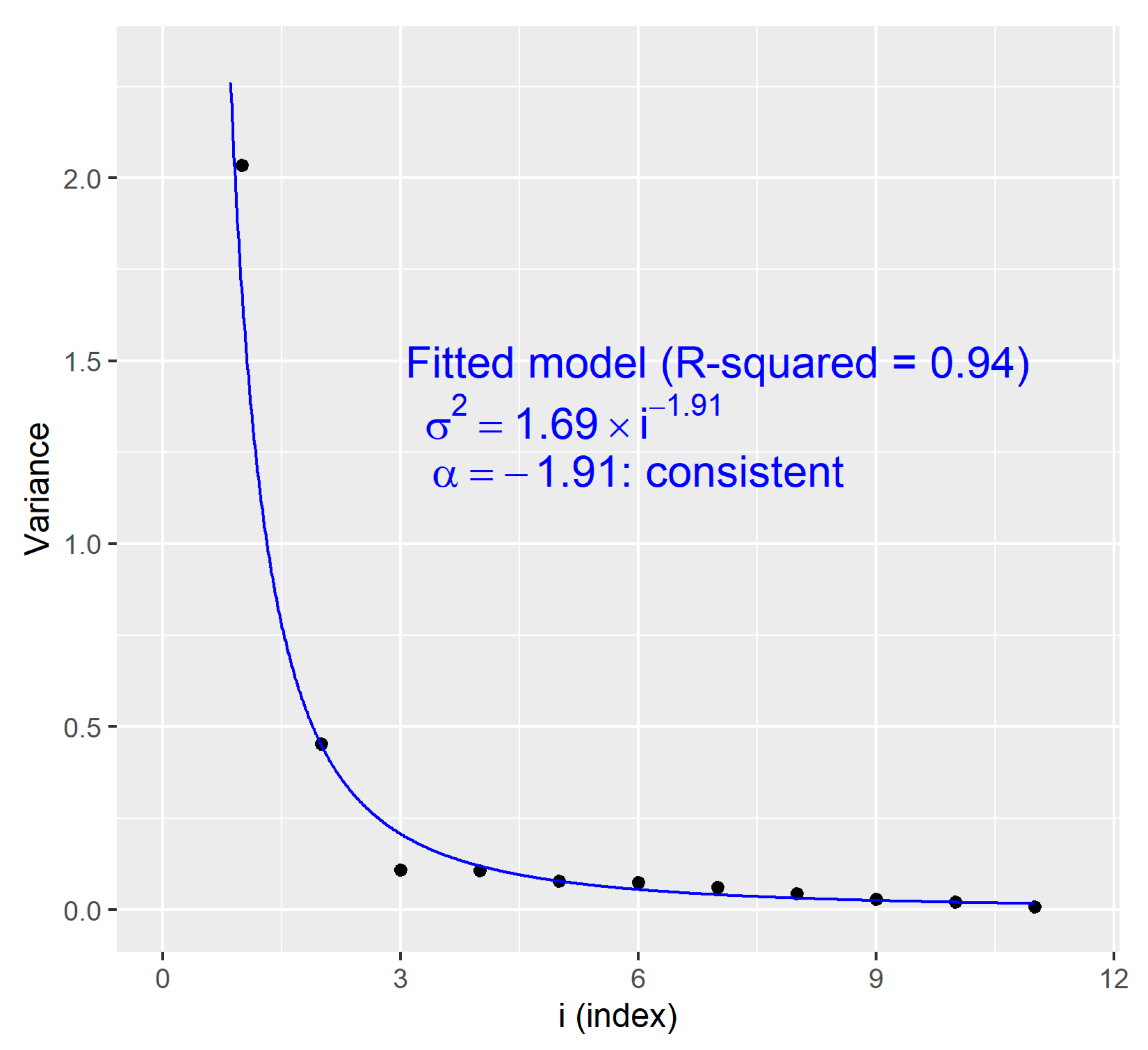
We applied Theorem 4 to examine the consistency of the estimator for this data example. We first fitted the model , where and . Figure 4 displays the observed value against the fitted value , where were obtained by the LSE for the decreasing sequence against . We observe that the LSE is fitted very well since the coefficient of determination (R-squared) is 0.94. That is, 94% of is explained by the model . Since is less than one, by Theorem 4, the estimator is consistent.
5. Extension to Unknown Variances
This section extends our theory (Section 3) to the case of unknown variances. Recall that we observe a random variable having the common mean and variance . . In this section, we assume that both and are unknown, where is estimated by (see Appendix A for an example for the estimator) and is estimated by
Unlike , the estimator entails additional variations by a random variable . Appendix A provides an example in which , where is the degree of freedom. This example corresponds to a meta-analysis, where is a mean difference and hence the pooled variance (Section 4.1). In this case, , and is independent of . The estimator is known as the Graybill-Deal estimator [25,26].
To show the consistency of , we apply Chebychev’s inequality conditional on the sequence , , … so that
Therefore, if the right-hand side goes to zero. The following theorem arises:
Theorem 5:
The common mean estimator is consistent if
6. Conclusions and Discussion
The literature has not explained regularity conditions for the consistency of estimating a common mean in fixed-effect meta-analyses, even though they provide a theoretical basis for meta-analyses. In this article, we provide five versions of regularity conditions (in Theorems 1–5) for making the common mean estimator to be consistent in fixed-effect meta-analyses. We conclude that, by well-regularizing the variances of studies, consistency can be achieved. On the other hand, we also reveal the conditions to make the estimator inconsistent, where the variances of studies fail to be regularized. These findings actually mean that readers better check the consistency when performing fixed-effect meta-analyses. For a more practical level, our findings facilitate the well-regularized variances by avoiding extremely small variances in studies.
We analyzed three real datasets to illustrate the main theorem (Theorem 4) that can determine the consistency or inconsistency of the common mean estimator via a simple linear model. The first and third datasets supported the consistency of the common mean estimator. On the other hand, the second data did not support the consistency of the estimator since the variances of the individual studies increased toward infinity too fast. The first dataset also exhibited increasing variances, yet its speed was slow enough to justify the consistency. The problem with the second data is that the meta-analysis accumulates more and more inaccurate studies. However, this inconsistency of the second example was stated solely for studies. Here, an implicit assumption is that the variances of the studies keep growing with . Unfortunately, this assumption cannot be checked only by a finite number of observed studies. Hence, our conclusion of the inconsistency becomes speculative.
An important future work is an extension of the consistency properties to bivariate, tri-variate, and multivariate meta-analyses [13,14,27,28,29]. Our current results on a univariate meta-analysis may not directly carry over to these multivariate settings since the estimator of the multivariate common means is no longer expressed as the weighted sum of the independent variables unless the multivariate normal distribution is imposed as in [29]. Instead, the estimator takes the form of the numerical maximization of the likelihood function [13,14,27,28]. The estimator becomes an even more complex form under some parameter restrictions [30,31]. Furthermore, the choice of parametric copulas is a key element in determining the form of the likelihood, such as the FGM copula [13], the Clayton copula [14], the Gaussian copula [28], and vine copulas [27], all of which were already adopted in meta-analyses. Other newly developed copulas not yet applied to meta-analysis can also be tried, such as the trigonometric copulas [32], generalized FGM copula [33], and Celebioglu–Cuadras copula [34]. More efforts are necessary to work on multivariate meta-analysis in order to establish the conditions/assumptions of the consistency of the multivariate common means.
Another important future work is an extension to fixed-effect meta-regression models, including fixed-effect structural equation models [1,5,27,35,36]. In the presence of explanatory variables, the common mean parameter could be written as a linear predictor. In these meta-regression models, regularity conditions for the consistency of regression coefficients were largely unexplored and, thus, should be clarified as we have in Theorems 1–5.
Supplementary Materials
The following supporting information can be downloaded at: https://www.mdpi.com/article/10.3390/axioms12050503/s1, the R code for the simulation and data analyses.
Author Contributions
Conceptualization, T.E.; formal analysis, N.T. and T.E.; funding acquisition, T.E.; methodology, N.T. and T.E.; supervision, T.E.; writing—original draft, N.T. and T.E. All authors have read and agreed to the published version of the manuscript.
Funding
This work was financially supported by JSPS KAKENHI (22K11948).
Institutional Review Board Statement
Not applicable.
Informed Consent Statement
Not applicable.
Data Availability Statement
All the results in this article are reproducible by the R code available in Supplementary Materials.
Acknowledgments
We thank the three reviewers for their helpful comments. We also thank Yoshihiko Konno (Department of Mathematics, Osaka Metropolitan University, Japan) for his helpful comments on theoretical properties and English corrections. We also thank Mihoko Mori (School of Medicine, Kurume University, Japan) for providing us with the allergic reaction data (Section 4.1).
Conflicts of Interest
The funders had no role in the design of the study; in the collection, analyses, or interpretation of data; in the writing of the manuscript; or in the decision to publish the results.
Appendix A. Pooled Variance Estimator
Recall that the mean difference is defined as , where is the j-th individual observation and is the sample size from the k-th group in the i-th study. We assume that . Then, , where is unbiasedly estimated by the pooled variance
Thus,
Appendix B
Proof of Theorem 3.
It can be shown that
where
is the distribution function of the standardized normal distribution. Therefore, the left-hand side of Equation (A1) is zero if . If , by the completeness axiom for an increasing and bounded sequence, for a real number . Therefore, the left-hand side of Equation (A1) is nonzero. □
Appendix C
Proof of Theorem 4.
Under the assumption of Theorem 4,
where is the Riemann zeta function. It is known that if and only if . Additionally, converges to a real number if . This completes the proof. □
References
- Borenstein, M.; Hedges, L.V.; Higgins, J.P.; Rothstein, H.R. Introduction to Meta-Analysis; John Wiley & Sons: Hoboken, NJ, USA, 2011. [Google Scholar]
- Kaiser, T.; Menkhoff, L. Financial Education in Schools: A Meta-analysis of Experimental Studies. Econ. Educ. Rev. 2020, 78, 101930. [Google Scholar] [CrossRef]
- Leung, Y.; Oates, J.; Chan, S.P. Voice, Articulation, and Prosody Contribute to Listener Perceptions of Speaker Gender: A Systematic Review and Meta-analysis. J. Speech Lang. Hear. Res. 2018, 61, 266–297. [Google Scholar] [CrossRef]
- DerSimonian, R.; Laird, N. Meta-analysis in Clinical Trials Revisited. Contemp. Clin. Trials 2015, 45, 139–145. [Google Scholar] [CrossRef]
- Fleiss, J.L. The Statistical Basis of Meta-analysis. Stat. Methods Med. Res. 1993, 2, 121–145. [Google Scholar] [CrossRef]
- Reyna-Villasmil, E.; Caponcello, M.G.; Maldonado, N.; Olivares, P.; Caroccia, N.; Bonazzetti, C.; Tazza, B.; Carrara, E.; Giannella, M.; Tacconelli, E.; et al. Association of Patients’ Epidemiological Characteristics and Comorbidities with Severity and Related Mortality Risk of SARS-CoV-2 Infection: Results of an Umbrella Systematic Review and Meta-Analysis. Biomedicines 2022, 10, 2437. [Google Scholar] [CrossRef]
- Pranata, R.; Lim, M.A.; Huang, I.; Raharjo, S.B.; Lukito, A.A. Hypertension is Associated with Increased Mortality and Severity of Disease in COVID-19 Pneumonia: A Systematic Review, Meta-analysis and Meta-regression. J. Renin-Angiotensin-Aldosterone Syst. 2020, 21, 1470320320926899. [Google Scholar] [CrossRef] [PubMed]
- Wang, Y.; Kala, M.P.; Jafar, T.H. Factors Associated with Psychological Distress During the Coronavirus Disease 2019 (COVID-19) Pandemic on the Predominantly General Population: A Systematic Review and Meta-analysis. PLoS ONE 2020, 15, e0244630. [Google Scholar] [CrossRef]
- Rice, K.; Higgins, J.P.; Lumley, T. A Re-evaluation of Fixed Effect (s) Meta-analysis. J. R. Stat. Soc. Ser. A 2018, 181, 205–227. [Google Scholar] [CrossRef]
- Lehmann, E.L. Elements of Large-Sample Theory; Springer Science & Business Media: Berlin, Germany, 2010. [Google Scholar]
- Serfling, R.J. Approximation Theorems of Mathematical Statistics; John Wiley & Sons: Hoboken, NY, USA, 1980. [Google Scholar]
- Shao, J. Mathematical Statistics; Springer Science & Business Media: New York, NY, USA, 2003. [Google Scholar]
- Shih, J.H.; Konno, Y.; Chang, Y.-T.; Emura, T. Estimation of a Common Mean Vector in Bivariate Meta-Analysis under the FGM copula. Statistics 2019, 53, 673–695. [Google Scholar] [CrossRef]
- Shih, J.H.; Konno, Y.; Chang, Y.T.; Emura, T. Copula-based Estimation Methods for a Common Mean Vector for Bivariate Meta-analyses. Symmetry 2002, 14, 186. [Google Scholar] [CrossRef]
- Shinozaki, N.; Chang, Y.T. Minimaxity of Empirical Bayes Estimators Shrinking Toward the Grand Mean when Variances are Unequal. Commun. Stat.-Theor. Methods 1996, 25, 183–199. [Google Scholar] [CrossRef]
- Singh, H.P.; Vishwakarma, G.K. A Family of Estimators of Population Mean Using Auxiliary Information in Stratified Sampling. Commun. Stat.-Theor. Methods 2008, 37, 1038–1050. [Google Scholar] [CrossRef]
- Malekzadeh, A.; Kharrati-Kopaei, M. Inferences on the Common Mean of Several Normal Populations under Hetero-scedasticity. Comput. Stat. 2018, 33, 1367–1384. [Google Scholar] [CrossRef]
- Bradley, R.A.; Gart, J.J. The Asymptotic Properties of ML Estimators when Sampling from Associated Populations. Biometrika 1962, 49, 205–214. [Google Scholar] [CrossRef]
- Emura, T.; Hu, Y.H.; Konno, Y. Asymptotic Inference for Maximum Likelihood Estimators under the Special Exponential Family with Double-truncation. Stat. Pap. 2017, 58, 877–909. [Google Scholar] [CrossRef]
- Kontopantelis, E.; Reeves, D. Performance of Statistical Methods for Meta-analysis when True Study Effects are Non-normally Distributed: A Simulation Study. Stat. Methods Med. Res. 2010, 21, 409–426. [Google Scholar] [CrossRef]
- Taketomi, N.; Konno, Y.; Chang, Y.T.; Emura, T. A Meta-analysis for Simultaneously Estimating Individual Means with Shrinkage, Isotonic Regression and Pretests. Axioms 2021, 10, 267. [Google Scholar] [CrossRef]
- Taketomi, N.; Michimae, H.; Chang, Y.T.; Emura, T. meta. Shrinkage: An R Package for Meta-analyses for Simultaneously Estimating Individual Means. Algorithms 2022, 15, 26. [Google Scholar] [CrossRef]
- Mori, M.; Kakuma, T. Development of a Prediction Model for Subjective Physical Symptoms Induced during Systematic Anatomy Practice among Medical Students. Kurume Med. J. 2023; in press. [Google Scholar]
- Dingena, C.F.; Arofikina, D.; Campbell, M.D.; Holmes, M.J.; Scott, E.M.; Zulyniak, M.A. Nutritional and Exercise-Focused Lifestyle Interventions and Glycemic Control in Women with Diabetes in Pregnancy: A Systematic Review and Meta-Analysis of Randomized Clinical Trials. Nutrients 2023, 15, 323. [Google Scholar] [CrossRef]
- Pal, N.; Lin, J.J.; Chang, C.H.; Kumar, S. A revisit to the common mean problem: Comparing the maximum likelihood estimator with the Graybill–Deal estimator. Comput. Stat. Data Anal. 2007, 51, 5673–5681. [Google Scholar] [CrossRef]
- Sinha, B.K.; Hartung, J.; Knapp, G. Statistical Meta-Analysis with Applications; John Wiley & Sons: Hoboken, NJ, USA, 2011. [Google Scholar]
- Nikoloulopoulos, A.K. A Multinomial Quadrivariate D-vine Copula Mixed Model for Meta-analysis of Diagnostic Studies in the Presence of Non-evaluable Subjects. Stat. Methods Med. Res. 2020, 29, 2988–3005. [Google Scholar] [CrossRef] [PubMed]
- Yamaguchi, Y.; Maruo, K. Bivariate Beta-binomial Model using Gaussian Copula for Bivariate Meta-analysis of Two Binary Outcomes with Low incidence. Jpn. J. Stat. Data. Sci. 2019, 2, 347–373. [Google Scholar] [CrossRef]
- Mavridis, D.; Salanti, G. A Practical Introduction to Multivariate Meta-analysis. Stat. Methods Med. Res. 2013, 22, 133–158. [Google Scholar] [CrossRef] [PubMed]
- Garg, N.; Misra, N. Estimation of Order Restricted Location/scale Parameters of a General Bivariate Distribution under General Loss Function: Some Unified Results. Jpn. J. Stat. Data. Sci. 2022, 5, 553–576. [Google Scholar] [CrossRef]
- Jena, P.; Ranjan Tripathy, M. Estimating Positive Powers of the Scale Parameters under Order Restriction for Two Normal Populations with a Common Mean. Statistics 2022, 56, 598–630. [Google Scholar] [CrossRef]
- Chesneau, C. Theoretical Study of Some Angle Parameter Trigonometric Copulas. Modelling 2022, 3, 140–163. [Google Scholar] [CrossRef]
- Susam, S.O. A multi-parameter Generalized Farlie-Gumbel-Morgenstern Bivariate Copula Family via Bernstein Polynomial. Hacet. J. Math. Stat. 2022, 51, 618–631. [Google Scholar] [CrossRef]
- Chesneau, C. Theoretical Contributions to Three Generalized Versions of the Celebioglu–Cuadras Copula. Analytics 2023, 2, 31–54. [Google Scholar] [CrossRef]
- Cheung, M.W.L.; Chan, W. Meta-analytic Structural Equation Modeling: A Two-stage Approach. Psychol. Methods 2005, 10, 40. [Google Scholar] [CrossRef]
- Standsyah, R.E.; Otok, B.W.; Suharsono, A. Fixed Effect Meta-Analytic Structural Equation Modeling (MASEM) Estimation Using Generalized Method of Moments (GMM). Symmetry 2021, 13, 2273. [Google Scholar] [CrossRef]
Figure 1.
The estimates for 0, based on with and under , , , , , and .
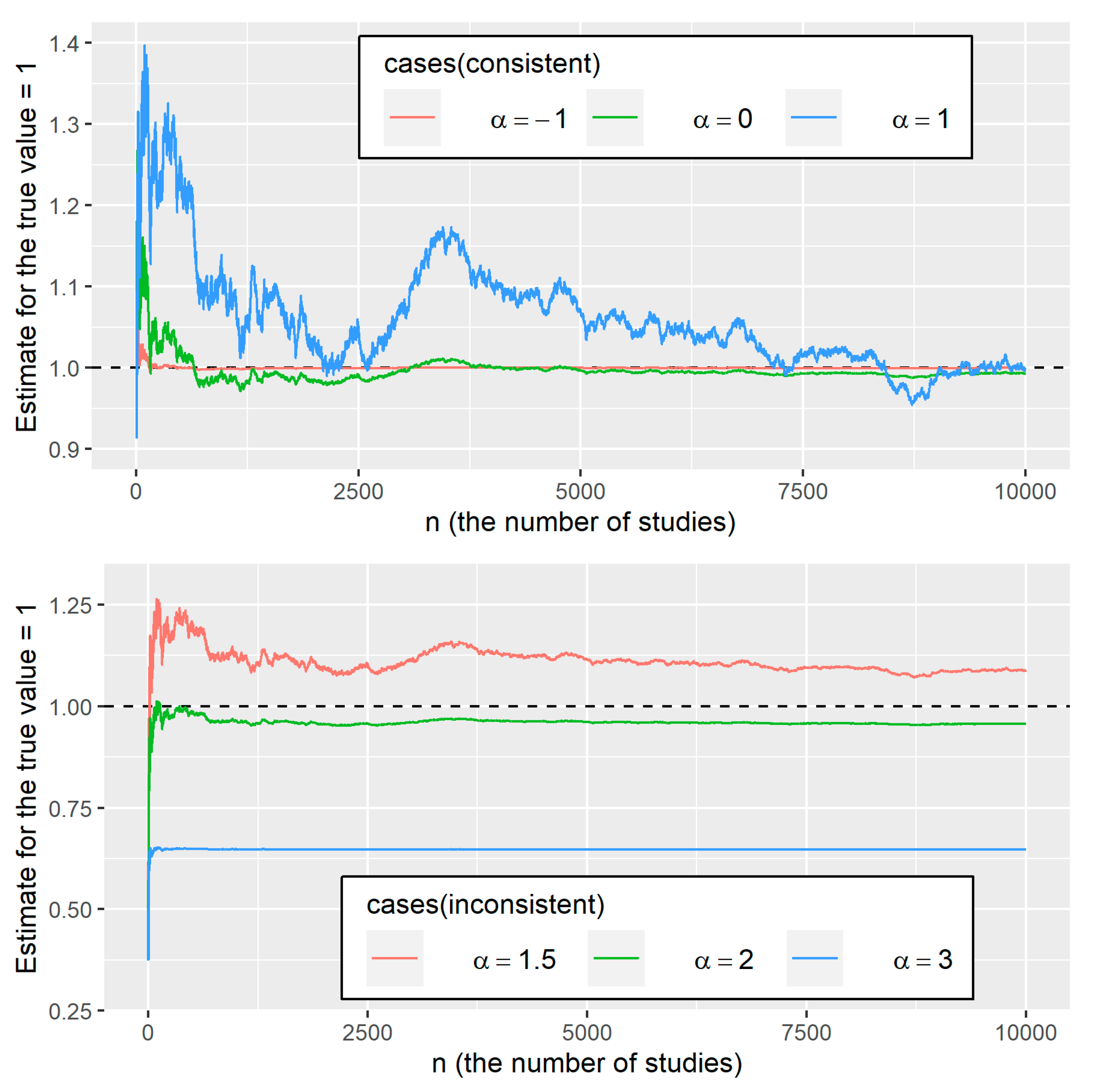
Figure 2.
Observed value vs. fitted value based on the allergic reaction data. The LSE was obtained for the sequence against .
Figure 2.
Observed value vs. fitted value based on the allergic reaction data. The LSE was obtained for the sequence against .

Figure 3.
Observed value vs. fitted value based on the diabetes data. The LSE was obtained for the increasing sequence against .
Figure 3.
Observed value vs. fitted value based on the diabetes data. The LSE was obtained for the increasing sequence against .
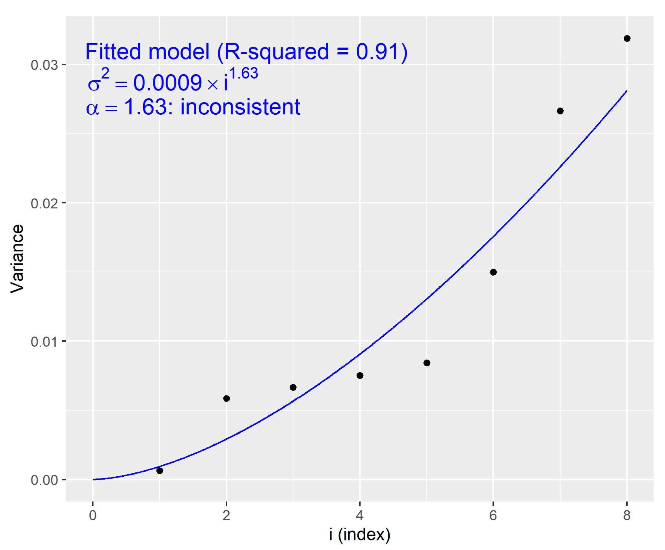
Figure 4.
Observed value vs. fitted value based on the COVID-19 data. The LSE were obtained for the decreasing sequence against .
Figure 4.
Observed value vs. fitted value based on the COVID-19 data. The LSE were obtained for the decreasing sequence against .

Table 1.
The dataset on the allergic reaction of medical students who were exposed to formaldehyde during an anatomy course [23].
Table 1.
The dataset on the allergic reaction of medical students who were exposed to formaldehyde during an anatomy course [23].
| i (Year) | Sample Size (Male) | Mean (Male) | SD (Male) | Sample Size (Female) | Mean (Female) | SD (Female) | MD | SE | SE2 |
|---|---|---|---|---|---|---|---|---|---|
| 1 (2015) | 74 | 5.09 | 1.59 | 42 | 5.26 | 1.65 | −0.17 | 0.3114 | 0.0970 |
| 2 (2016) | 79 | 4.84 | 1.62 | 37 | 5.42 | 1.69 | −0.58 | 0.3272 | 0.1071 |
| 3 (2018) | 79 | 4.81 | 1.54 | 34 | 5.26 | 1.69 | −0.45 | 0.3253 | 0.1058 |
| 4 (2019) | 74 | 4.86 | 1.62 | 33 | 5.61 | 1.58 | −0.75 | 0.3366 | 0.1133 |
| 5 (2022) | 73 | 4.79 | 1.68 | 37 | 5.35 | 1.83 | −0.56 | 0.3494 | 0.1221 |
NOTE: Sample sizes are the number of medical students. Means are the mean scores. SDs are the standard deviations of the scores. MD is the mean difference between male and female (male–female) scores. SE is computed as the square root of the pooled variance using the SDs of male and female groups.
Table 2.
The summary of 8 studies that examined the mean difference (MD) between the intervention group and the control group for pregnant women with diabetes [24].
Table 2.
The summary of 8 studies that examined the mean difference (MD) between the intervention group and the control group for pregnant women with diabetes [24].
| Study | Sample Size | (mmol/L) | SE | |
|---|---|---|---|---|
| Aslfalah 2020 | 60 | −0.70 | 0.0256 | 0.0007 |
| Fei 2014 | 97 | −0.47 | 0.1224 | 0.0150 |
| Hajimoosayi 2020 | 70 | −0.20 | 0.0816 | 0.0067 |
| Jamilian 2018 | 40 | −0.40 | 0.1786 | 0.0319 |
| Jamilian 2019 | 60 | −0.10 | 0.0765 | 0.0059 |
| Jamilian 2020 | 51 | −0.33 | 0.0918 | 0.0084 |
| Lindsay 2015 | 100 | 0.01 | 0.0867 | 0.0075 |
| Ostadmohammadi 2019 | 54 | −0.20 | 0.1633 | 0.0267 |
NOTE: Sample sizes are the number of pregnant women with diabetes. MD is the mean difference between the intervention group and the control group. SE is the standard error of the ML.
Table 3.
Summary of the 11 studies (shown by the author and publication year) on COVID-19 patients for examining the effects of hypertension on mortality.
Table 3.
Summary of the 11 studies (shown by the author and publication year) on COVID-19 patients for examining the effects of hypertension on mortality.
| Study | Sample Size | log (RR) | SE | SE2 |
|---|---|---|---|---|
| Akbari 2020 | 440 | 0.6881 | 0.6732 | 0.4532 |
| Bai 2000 | 127 | 0.5933 | 0.2754 | 0.0758 |
| Cao 2020 | 102 | 1.1756 | 0.2821 | 0.0796 |
| Chen 2020 | 123 | 0.5365 | 0.2493 | 0.0621 |
| Chen T 2020 | 274 | 0.6780 | 0.1713 | 0.0294 |
| Fu 2020 | 200 | 0.5878 | 0.3302 | 0.1090 |
| Grasselli 2020 | 1591 | 0.4637 | 0.0956 | 0.0091 |
| Li 2020 | 102 | 0.5247 | 0.3272 | 0.1071 |
| Luo 2020 | 403 | 1.2326 | 0.1489 | 0.0222 |
| Yuan 2020 | 27 | 2.8904 | 1.4263 | 2.0344 |
| Zhou 2020 | 191 | 1.1378 | 0.2097 | 0.0440 |
NOTE: Sample sizes are the number of patients with COVID-19. log (RR) is the log of the risk ratio for examining the association (mortality vs. hypertension). SE is the standard error of the log (RR). SE is the standard error of the log (RR).
Disclaimer/Publisher’s Note: The statements, opinions and data contained in all publications are solely those of the individual author(s) and contributor(s) and not of MDPI and/or the editor(s). MDPI and/or the editor(s) disclaim responsibility for any injury to people or property resulting from any ideas, methods, instructions or products referred to in the content. |
© 2023 by the authors. Licensee MDPI, Basel, Switzerland. This article is an open access article distributed under the terms and conditions of the Creative Commons Attribution (CC BY) license (https://creativecommons.org/licenses/by/4.0/).
Share and Cite
MDPI and ACS Style
Taketomi, N.; Emura, T. Consistency of the Estimator for the Common Mean in Fixed-Effect Meta-Analyses. Axioms 2023, 12, 503. https://doi.org/10.3390/axioms12050503
AMA Style
Taketomi N, Emura T. Consistency of the Estimator for the Common Mean in Fixed-Effect Meta-Analyses. Axioms. 2023; 12(5):503. https://doi.org/10.3390/axioms12050503
Chicago/Turabian StyleTaketomi, Nanami, and Takeshi Emura. 2023. "Consistency of the Estimator for the Common Mean in Fixed-Effect Meta-Analyses" Axioms 12, no. 5: 503. https://doi.org/10.3390/axioms12050503
Note that from the first issue of 2016, this journal uses article numbers instead of page numbers. See further details here.