

A Fractional Analysis of Zakharov–Kuznetsov Equations with the Liouville–Caputo Operator

1
Basic Science Department, College of Science and Theoretical Studies, Saudi Electronic University, Riyadh 11673, Saudi Arabia
2
Department of Mathematical Sciences, College of Sciences, Princess Nourah bint Abdulrahman University, Riyadh 11546, Saudi Arabia
3
Department of Mathematics, Abdul Wali Khan University Mardan, Mardan 23200, Pakistan
*
Author to whom correspondence should be addressed.
Axioms 2023, 12(6), 609; https://doi.org/10.3390/axioms12060609
Submission received: 30 April 2023
/
Revised: 11 June 2023
/
Accepted: 17 June 2023
/
Published: 19 June 2023
(This article belongs to the Special Issue New Trends in Fractional Operators with Applications in Mathematical Physics)
Abstract
:In this study, we used two unique approaches, namely the Yang transform decomposition method (YTDM) and the homotopy perturbation transform method (HPTM), to derive approximate analytical solutions for nonlinear time-fractional Zakharov–Kuznetsov equations (ZKEs). This framework demonstrated the behavior of weakly nonlinear ion-acoustic waves in plasma containing cold ions and hot isothermal electrons in the presence of a uniform magnetic flux. The density fraction and obliqueness of two compressive and rarefactive potentials are depicted. In the Liouville–Caputo sense, the fractional derivative is described. In these procedures, we first used the Yang transform to simplify the problems and then applied the decomposition and perturbation methods to obtain comprehensive results for the problems. The results of these methods also made clear the connections between the precise solutions to the issues under study. Illustrations of the reliability of the proposed techniques are provided. The results are clarified through graphs and tables. The reliability of the proposed procedures is demonstrated by illustrative examples. The proposed approaches are attractive, though these easy approaches may be time-consuming for solving diverse nonlinear fractional-order partial differential equations.
Keywords:
Yang transform; fractional Zakharov–Kuznetsov equations; Liouville–Caputo operator; Adomian decomposition method (ADM); homotopy perturbation method (HPM)MSC:
34A25; 34A08; 26A33; 35A201. Introduction
The generalization of integer-order to arbitrary-order calculus is known as fractional calculus (FC), and it was first developed around the end of the seventeenth century. The main advantage of fractional calculus is that it has been shown to be a highly useful tool for understanding the memory and hereditary characteristics of numerous phenomena. Additionally, ordinary calculus represents a small subset of fractional calculus. The fractional-order derivative groundwork was laid through the combined effort of pioneers such as Riemann [1], Liouville [2], Caputo [3], Podlubny [4], and Miller and Ross [5], among many others [6,7]. The early theory of fractional derivatives has been rapidly advanced throughout the past few decades. Authors such as Srivastava [8], Kilbas et al. [9], Legnani et al. [10], and Hilfer [11] have gone into additional detail and developed the area. The main focus of their studies was the systematic comprehension of FC, including uniqueness and existence. The theory of fractional-order calculus has been linked to real-world projects and used in a variety of fields, including electrodynamics [12], chaos theory [13], optics [14], signal processing [15], and other areas [16,17,18,19,20,21,22].
The aforementioned works played a crucial role in our understanding of the nature and behavior of nonlinear problems that arise in daily life, as well as the analytical and numerical solutions for differential equations of an arbitrary order. Through spatial and temporal fractional-order derivatives, fractional-order models have expanded our understanding of differentiability and added nonlocal and system memory effects. These characteristics enable us to model phenomena at various temporal and spatial scales without dividing the problem into even more subsets. The assumption that fractional derivatives can highlight or capture key characteristics of complicated events is the foundation for using fractional-order models to span various scales. Furthermore, because classical derivatives are local in nature, we can only use them to describe changes in a point’s immediate surroundings; however, fractional derivatives allow us to express changes in an interval. Because of this characteristic, arbitrary-order derivatives can be used to model a wider range of physical processes related to quantum physics, signal analysis, diffusion, elasticity, and seismic vibrations. It has been discovered that fractional differential equations may explain many systems in transdisciplinary fields more effectively and conveniently. Fractional derivatives are now frequently employed to examine a variety of difficult issues. For instance, fractional calculus is used for the mathematical modeling of viscoelastic materials [23].
It is becoming noticeable that fractional partial differential equations (FPDEs) are a useful modeling tool for complicated multiscale events, particularly those combining overlapping microscopic and macroscopic dimensions. In contrast to integer-order PDEs, the fractional order of the derivatives in FPDEs can be a function of both space and time or even distribution. This has created outstanding prospects for simulating and modeling multi-physics phenomena, such as the smooth transition from wave propagation to diffusion or from local to non-local dynamics. Numerous well-known scholars have made contributions to this area due to the importance of analytically solving FPDEs in engineering and science [24,25,26,27,28,29]. With the aid of the Elzaki transform decomposition approach, the approximate analytical solution for time-fractional Swift–Hohenberg equations with conformable derivatives was studied in [30]. The authors of [31] used the natural decomposition approach to obtain the solutions of the fractional modified Boussinesq and approximate long wave equations. In [32], a new fractional sub-equation method was used to study an exact solution for fractional partial differential equations. A new analytical solution for fractional nonlinear systems of third-order Korteweg–de Vries (KdV) equations and systems of coupled Burgers equations in one and two dimensions were investigated by the variational iteration method in [33] using a conformable fractional derivative. Fractional calculus has been used by many scholars as a tool to ascertain the nature of complex problems [34,35,36,37,38,39,40,41].
The Korteweg–de Vries equations are essential for scientific applications. One of the well-known variations are the ZKEs, which analyze electrostatic-acoustic pulses in magnetized ions. They were developed in an ocean-based study of coastal waves [42]. To show nonlinear phenomena such as isotope waves in high-magnetization lossless plasma, the ZKEs were initially developed in two dimensions [43]. In this study, we investigated the time-fractional Zakharov–Kuznetsov (FZK) equation ) with a fractional time-derivative of the order , possessing the following form:
where , denotes the Liouville–Caputo fractional derivative of the order and are arbitrary constants; are integers; and the nature of nonlinear events such as ion-acoustic waves in the context of a symmetrical magnetic field in plasma containing hot isothermal electrons and cold ions is depicted by the expression [44,45]. The ZKEs were suggested to examine a shallow nonlinear isotope ripple in a plasma with significant magnetization impairment in three dimensions by the authors of [43]. The variation iteration method [46] and the HPM [47] have been used, respectively, to examine the approximative analytical solutions of fractional ZKEs. Several of the above-mentioned strategies suffered from the drawback that they were invariably hierarchical and involved a great deal of computational complexity. The innovations of this research are the YTDM and HPTM, which combine the Yang transform (YT), ADM, and HPM to solve the time-fractional ZKE. The Yang transform was introduced by Xiao-Jun Yang and can be used to handle various kinds of differential equations with constant coefficients [48]. The proposed method made it simpler to estimate the series terms as compared to the traditional Adomian process [49,50], since it does not need to compute the fractional derivative or fractional integrals in the recursive mechanism. Since the YTDM does not require prescribed assumptions, linearization, discretization, or perturbation, round-off errors are avoided. In the literature, the YTDM has been used to solve a wide range of differential equations, including Lax’s time-fractional Korteweg–de Vries equation [51] and the phi-four equations [52]. He’s polynomials, the Yang transform, and the homotopy perturbation method have been combined to generate the HPTM [53,54,55]. He’s polynomials can be applied to simply manage nonlinear terms. The proposed method’s analytical results demonstrated how easily implemented and highly desirable this method is computationally. It appears that these new methods could be used to reduce the time and cost of computing. The abovementioned methods produce convergent series.
The remainder of this article is structured as follows. We introduce some definitions and YT features in Section 2. We describe the suggested methods for resolving fractional partial differential equations (FPDEs) in Section 3 and Section 4. After that, in Section 5, we use the methods discussed to find approximations of solutions to the fractional space-time ZK equation. In Section 6, we discuss the numerical simulations for present methods. The paper’s conclusions are stated in Section 7.
2. Preliminaries
For our analysis, a number of definitions and axiom results from the literature were necessary.
Definition 1.
The fractional Liouville–Caputo derivative is as follows [56]:
Definition 2.
Some important functions for the YT are stated as follows:
representing the inverse YT as
Definition 3.
The YT of the stated function with a derivative of nth order is given as follows [48]:
Definition 4.
The YT of the stated function with derivative of order fractional is given as [48]
3. Configuration for HPTM
In this subsection, we explain the basic concept behind the HPTM for solving the FPDE:
with the initial guesses
Here, denotes the Liouville–Caputo fractional derivative, and and are linear and nonlinear operators, respectively.
Upon implementing the YT, we have
which yields
By utilizing the inverse YT, we obtain
Utilizing the HPM, we obtain
with the parameter .
The nonlinear term is taken as
In addition, describes He’s polynomials and is written as follows:
where
Substituting (12) and (13) into (11), we obtain
On comparing the coefficients on both sides, we obtain
Lastly, the approximate analytical solution is stated as
4. Configuration for YTDM
In this subsection, we illustrate the basic concept behind the YTDM for solving the FPDE:
with the initial guesses
Here, denotes the Liouville–Caputo fractional derivative, and and are linear and nonlinear operators, respectively.
Upon implementing the YT, we have
which yields
By utilizing the inverse YT, we obtain
Utilizing the YTDM, we have
The nonlinear term is taken as
with
Substituting (22) and (23) into (21), we obtain
Thus, we obtain the following approximation:
In general, for , we can write
5. Numerical Applications
Example 1.
Let us assume a nonlinear FZK equation of the form
with the initial guess
Upon implementing the YT, we have
which yields
By utilizing the inverse YT, we obtain
Utilizing the HPM, we obtain
In addition, the nonlinear terms obtained by means of He’s polynomial are as follows:
Some nonlinear terms are presented as below:
On comparing the ϵ coefficients on both sides, we obtain
The approximate analytical solution obtained by means of the HPTM is as follows:
Implementation of YTDM
Upon implementing the YT, we have
which yields
By utilizing the inverse YT, we obtain
Utilizing the YTDM, we have
The nonlinear term obtained by means of the Adomian polynomial is taken as . Thus, we obtain
Some nonlinear terms are presented below:
Thus, we obtain the following approximation:
For
For
For
Consequently, we determine the series solutions by continuing the same process in order to calculate the components for as follows:
By setting , we obtain
Example 2.
Let us assume a nonlinear FZK equation of the form
with the initial guess
Upon implementing the YT, we have
which yields
By utilizing the inverse YT, we obtain
Utilizing the HPM, we obtain
In addition, the nonlinear terms obtained by means of He’s polynomial are as follows:
Some nonlinear terms are presented below:
On comparing the ϵ coefficients on both sides, we obtain
The approximate analytical solution obtained by means of the HPTM is as follows:
Implementation of YTDM
Upon implementing the YT, we have
which yields
By utilizing the inverse YT, we obtain
Utilizing the YTDM, we have
The nonlinear term obtained by means of the Adomian polynomial is taken as . Thus, we have
Some nonlinear terms are presented below:
Thus, we obtain the following approximation:
For
For
Consequently, we determine the series solutions by continuing the same process in order to calculate the components for as follows:
By setting , we obtain
6. Numerical Simulation Studies
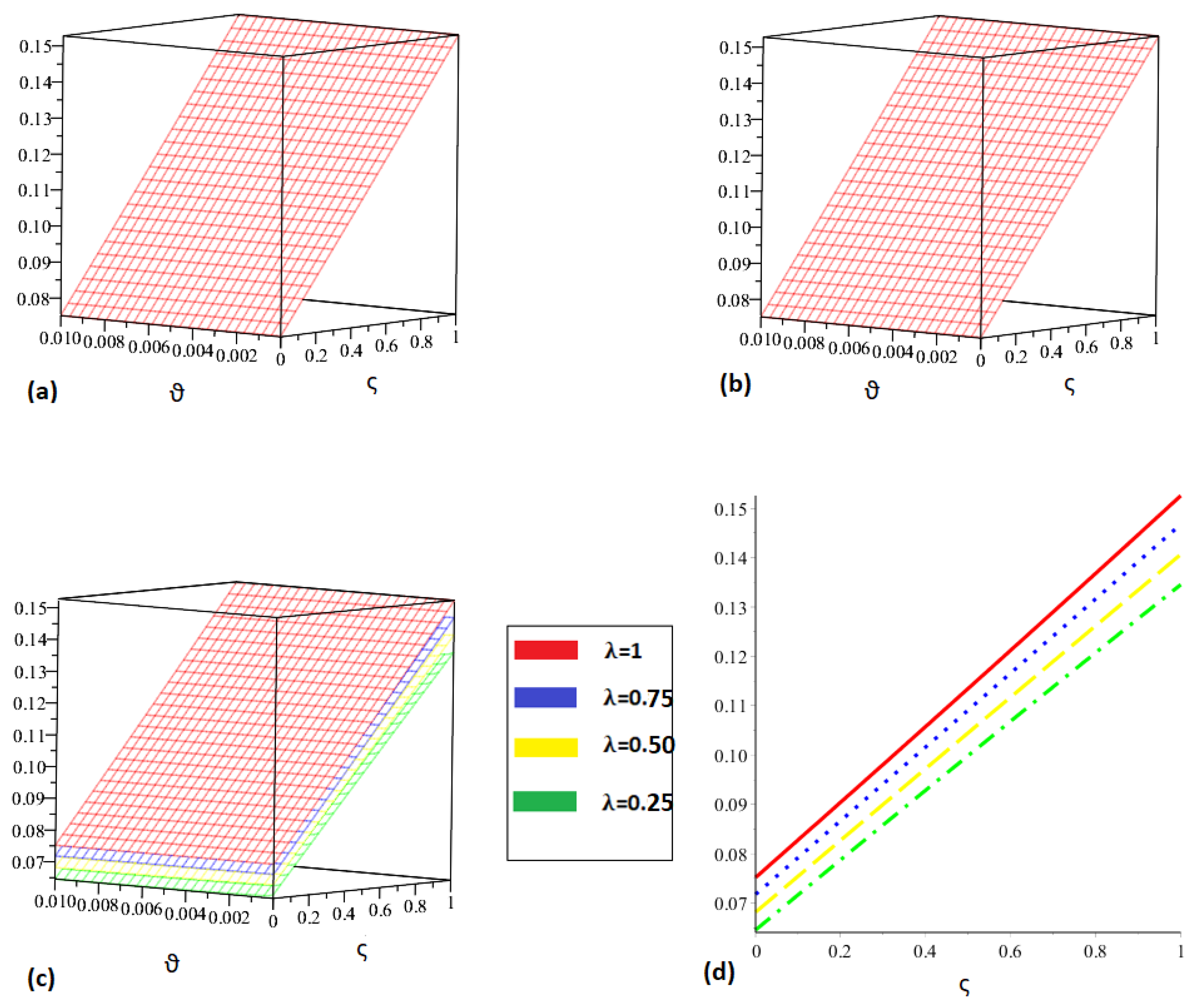
In this section, we present a numerical analysis to verify the precision of the numerical solution obtained by the two effective techniques. The third-order series solution was taken into consideration to assess the corresponding behavior in the proposed approaches. Figure 1a shows the behavior of the exact solution, while Figure 1b shows the graphical behavior for the approximative solution derived using the proposed approaches with . A surface plot of approximations for various fractional orders with , and 1 is shown in Figure 1c,d for . We illustrate the behavior of the exact solution in Figure 2a and the graphical behavior of the approximative solution derived by the proposed approaches in Figure 2b for . Similarly, the surface plot of approximations for various fractional orders with , and 1 is shown in Figure 2c,d for . The domains for all the figures are , , with and . A comparison of the exact and approximative solutions for various values of is shown in Table 1. In Table 2, we compare our solution with the solutions derived by the perturbation–iteration algorithm (PIA) and residual power series method (RPSM) in terms of absolute error at and , as an example. Table 3 represents the comparison between the exact and the approximate solution for various values of , whereas in Table 4 we compare our solution with the solution derived by the variational iteration method (VIM) in terms of absolute error at and , as an example. The numerical simulation is presented to show the precision and demonstrate how the resulting solution converged to the exact solution as the fractional order transitioned into the classical order. Finally, we can conclude that the analysis under consideration could help researchers better understand the nature of various nonlinear and complex problems describing a variety of events. Both the couple and the system of equations describing real-world situations could be solved using the proposed techniques and fractional operator.
7. Conclusions
The time-fractional ZK equation, which governs the nonlinear evolution of ion-acoustic waves in a magnetized plasma with hot and cold electrons, was investigated in this study using the proposed YTD and HPT methods. Both negative (rarefactive) and positive (compressive) potential structures that were symmetric about the origin were produced according to the different physical properties. Due to the limited number of estimations used in the proposed procedures, they were more effective than alternative analytical approaches. We gained a clear understanding of the technique, because it entailed directly applying the YT to the anticipated problem before modifying the ADM and HPM. The approximate solution to the considered problem was then derived using the inverse Yang transform. We presented 2D and 3D plots to illustrate the compatibility of the generated model and the precise solutions to the problems, respectively. The results obtained by existing studies were very well in line with the solutions presented in examples 1 and 2 in this paper. The simulations demonstrated that the proposed techniques attained remarkable agreement, suggesting that the proposed methods are quite effective and simple to use for obtaining approximative analytical solutions to a variety of fractional physical and biological models.
Author Contributions
Conceptualization, A.H.G., F.M. and A.K.; methodology, A.H.G., F.M. and A.K.; software, A.K.; validation, A.H.G., F.M. and A.K.; formal analysis, A.K.; investigation, A.K.; resources, A.H.G., F.M. and A.K.; data curation, A.H.G., A.K.; writing—original draft preparation, A.K.; writing—review and editing, A.K.; visualization, A.H.G., A.K.; supervision, A.H.G., F.M.; project administration, F.M.; funding acquisition, F.M. All authors have read and agreed to the published version of the manuscript.
Funding
This research received no external funding.
Data Availability Statement
The numerical data used to support the findings of this study are included within the article.
Acknowledgments
We would like to thank the reviewers for their careful reading of our paper and constructive suggestions for improving its quality. Additionally, the author Fatemah Mofarreh expresses her gratitude to the Princess Nourah bint Abdulrahman University Researcher Support Project (number PNURSP2023R27), Princess Nourah bint Abdulrahman University, Riyadh, Saudi Arabia.
Conflicts of Interest
The authors declare no conflict of interest.
References
- Riemann, G.F.B. Versuch einer allgemeinen Auffassung der Integration und Differentiation, Gesammelte Mathematische Werke; Springer: Leipzig, Germany, 1896. [Google Scholar]
- Liouville, J. Memoire sur quelques questions de geometrie et de mecanique, et sur un nouveau genre de calcul pour resoudre ces questions. J. Ecole Polytech. 1832, 13, 1–69. [Google Scholar]
- Caputo, M. Elasticita e Dissipazione; Zanichelli: Bologna, Italy, 1969. [Google Scholar]
- Podlubny, I. Fractional Differential Equations; Academic Press: New York, NY, USA, 1999. [Google Scholar]
- Miller, K.S.; Ross, B. An Introduction to Fractional Calculus and Fractional Differential Equations; Wiley: New York, NY, USA, 1993. [Google Scholar]
- Sene, N.; Abdelmalek, K. Analysis of the fractional diffusion equations described by Atangana-Baleanu-Caputo fractional derivative. Chaos Solitons Fractals 2019, 127, 158–164. [Google Scholar] [CrossRef]
- Murio, D.A. Stable numerical evaluation of Grünwald-Letnikov fractional derivatives applied to a fractional IHCP. Inverse Probl. Sci. Eng. 2009, 17, 229–243. [Google Scholar] [CrossRef]
- Srivastava, H.M. Some parametric and argument variations of the operators of fractional calculus and related special functions and integral transformations. J. Nonlinear Convex Anal. 2021, 22, 1501–1520. [Google Scholar]
- Kilbas, A.A.; Srivastava, H.M.; Trujillo, J.J. Theory and Applications of Fractional Differential Equations; Elsevier: Amsterdam, The Netherlands, 2006; Volume 204. [Google Scholar]
- Legnani, W.; Moschandreou, T.E.; Reyhanoglu, M. Nonlinear Systems: Theoretical Aspects and Recent Applications; IntechOpen: London, UK, 2020. [Google Scholar]
- Hilfer, R. (Ed.) Applications of Fractional Calculus in Physics; World Scientific: Singapore, 2000. [Google Scholar]
- Nasrolahpour, H. A note on fractional electrodynamics. Commun. Nonlinear Sci. Numer. Simul. 2013, 18, 2589–2593. [Google Scholar] [CrossRef]
- Lin, W. Global existence theory and chaos control of fractional differential equations. J. Math. Anal. Appl. 2007, 332, 709–726. [Google Scholar] [CrossRef] [Green Version]
- Esen, A.; Sulaiman, T.A.; Bulut, H.; Baskonus, H.M. Optical solitons and other solutions to the conformable space-time fractional Fokas-Lenells equation. Optik 2018, 167, 150–156. [Google Scholar] [CrossRef]
- Li, Y.; Liub, F.; Turner, I.W.; Li, T. Time-fractional diffusion equation for signal smoothing. Appl. Math. Comput. 2018, 326, 108–116. [Google Scholar] [CrossRef] [Green Version]
- Al-Smadi, M.; Freihat, A.; Khalil, H.; Momani, S.; Ali Khan, R. Numerical multistep approach for solving fractional partial differential equations. Int. J. Comput. Methods 2017, 14, 1750029. [Google Scholar] [CrossRef]
- Sheng, H.; Chen, Y.; Qiu, T. Fractional Processes and Fractional-Order Signal Processing: Techniques and Applications; Springer Science & Business Media: Berlin, Germany, 2011. [Google Scholar]
- Sunthrayuth, P.; Alyousef, H.A.; El-Tantawy, S.A.; Khan, A.; Wyal, N. Solving Fractional-Order Diffusion Equations in a Plasma and Fluids via a Novel Transform. J. Funct. Spaces 2022, 2022, 1899130. [Google Scholar] [CrossRef]
- Shah, N.A.; El-Zahar, E.R.; Akgül, A.; Khan, A.; Kafle, J. Analysis of fractional-order regularized long-wave models via a novel transform. J. Funct. Spaces 2022, 2022, 2754507. [Google Scholar] [CrossRef]
- Rezapour, S.; Etemad, S.; Tellab, B.; Agarwal, P.; Garcia Guirao, J.L. Numerical solutions caused by DGJIM and ADM methods for multi-term fractional BVP involving the generalized ψ-RL-operators. Symmetry 2021, 13, 532. [Google Scholar] [CrossRef]
- Amara, A.; Etemad, S.; Rezapour, S. Approximate solutions for a fractional hybrid initial value problem via the Caputo conformable derivative. Adv. Differ. Equ. 2020, 2020, 608. [Google Scholar] [CrossRef]
- Etemad, S.; Shikongo, A.; Owolabi, K.M.; Tellab, B.; Avci, I.; Rezapour, S.; Agarwal, R.P. A new fractal-fractional version of giving up smoking model: Application of Lagrangian piece-wise interpolation along with asymptotical stability. Mathematics 2022, 10, 4369. [Google Scholar] [CrossRef]
- Ogata, K. Modern Control Engineering; Prentice Hall: Upper Saddle River, NJ, USA, 2010; Volume 5. [Google Scholar]
- Owyed, S.; Abdou, M.A.; Abdel-Aty, A.H.; Alharbi, W.; Nekhili, R. Numerical and approximate solutions for coupled time fractional nonlinear evolutions equations via reduced differential transform method. Chaos Solitons Fractals 2020, 131, 109474. [Google Scholar] [CrossRef]
- Song, L.; Zhang, H. Application of homotopy analysis method to fractional KdV-Burgers-Kuramoto equation. Phys. Lett. A 2007, 367, 88–94. [Google Scholar] [CrossRef]
- Arqub, O.A.; El-Ajou, A. Solution of the fractional epidemic model by homotopy analysis method. J. King Saud Univ.-Sci. 2013, 25, 73–81. [Google Scholar] [CrossRef] [Green Version]
- Das, S.; Vishal, K.; Gupta, P.K.; Yildirim, A. An approximate analytical solution of time-fractional telegraph equation. Appl. Math. Comput. 2011, 217, 7405–7411. [Google Scholar] [CrossRef]
- Jassim, H.K.; Shareef, M.A. On approximate solutions for fractional system of differential equations with Caputo-Fabrizio fractional operator. J. Math. Comput. Sci. 2021, 23, 58–66. [Google Scholar] [CrossRef]
- Mahor, T.C.; Mishra, R.; Jain, R. Analytical solutions of linear fractional partial differential equations using fractional Fourier transform. J. Comput. Appl. Math. 2021, 385, 113202. [Google Scholar] [CrossRef]
- Nonlaopon, K.; Alsharif, A.M.; Zidan, A.M.; Khan, A.; Hamed, Y.S.; Shah, R. Numerical investigation of fractional-order Swift-Hohenberg equations via a Novel transform. Symmetry 2021, 13, 1263. [Google Scholar] [CrossRef]
- Botmart, T.; Agarwal, R.P.; Naeem, M.; Khan, A.; Shah, R. On the solution of fractional modified Boussinesq and approximate long wave equations with non-singular kernel operators. AIMS Math. 2022, 7, 12483–12513. [Google Scholar] [CrossRef]
- Zheng, B.; Wen, C. Exact solutions for fractional partial differential equations by a new fractional sub-equation method. Adv. Differ. Equ. 2013, 2013, 199. [Google Scholar] [CrossRef] [Green Version]
- Alderremy, A.A.; Aly, S.; Fayyaz, R.; Khan, A.; Shah, R.; Wyal, N. The analysis of fractional-order nonlinear systems of third order KdV and Burgers equations via a novel transform. Complexity 2022, 2022, 4935809. [Google Scholar] [CrossRef]
- Ganie, A.H.; AlBaidani, M.M.; Khan, A. A Comparative Study of the Fractional Partial Differential Equations via Novel Transform. Symmetry 2023, 15, 1101. [Google Scholar] [CrossRef]
- Al-Sawalha, M.M.; Khan, A.; Ababneh, O.Y.; Botmart, T. Fractional view analysis of Kersten-Krasil’shchik coupled KdV-mKdV systems with non-singular kernel derivatives. AIMS Math. 2022, 7, 18334–18359. [Google Scholar] [CrossRef]
- Ganie, A.H.; Houas, M.; AlBaidani, M.M.; Fathima, D. Coupled system of three sequential Caputo fractional differential equations: Existence and stability analysis. Math. Methods Appl. Sci. 2023. early view. [Google Scholar] [CrossRef]
- AL-Smadi, M.H.; Gumah, G.N. On the homotopy analysis method for fractional SEIR epidemic model. Res. J. Appl. Sci. Eng. Technol. 2014, 7, 3809–3820. [Google Scholar] [CrossRef]
- Kolokoltsov, V.N. The probabilistic point of view on the generalized fractional partial differential equations. Fract. Calc. Appl. Anal. 2019, 22, 543–600. [Google Scholar] [CrossRef] [Green Version]
- Martin, O. Stability approach to the fractional variational iteration method used for the dynamic analysis of viscoelastic beams. J. Comput. Appl. Math. 2019, 346, 261–276. [Google Scholar] [CrossRef]
- Khader, M.; Kumar, S.; Abbasbandy, S. Fractional homotopy analysis transforms method for solving a fractional heat-like physical model. Walailak J. Sci. Technol. (WJST) 2016, 13, 337–353. [Google Scholar]
- Haq, F.; Shah, K.; ur Rahman, G.; Shahzad, M. Numerical solution of fractional order smoking model via Laplace Adomian decomposition method. Alex. Eng. J. 2018, 57, 1061–1069. [Google Scholar] [CrossRef]
- Çenesiz, Y.; Tasbozan, O.; Kurt, A. Functional Variable Method for conformable fractional modified KdV-ZK equation and Maccari system. Tbilisi Math. J. 2017, 10, 117–125. [Google Scholar] [CrossRef]
- Zakharov, V.; Kuznetsov, E. On three-dimensional solitons. Sov. Phys. 1974, 39, 285–288. [Google Scholar]
- Monro, S.; Parkes, E.J. The derivation of a modified Zakharov-Kuznetsov equation and the stability of its solutions. J. Plasma Phys. 1999, 62, 305–317. [Google Scholar] [CrossRef]
- Monro, S.; Parkes, E.J. Stability of solitary-wave solutions to a modified Zakharov-Kuznetsov equation. J. Plasma Phys. 2000, 64, 41126. [Google Scholar] [CrossRef]
- Molliq, R.Y.; Noorani, M.S.M.; Hashim, I.; Ahmad, R.R. Approximate solutions of fractional Zakharov-Kuznetsov equations by VIM. J. Comput. Appl. Math. 2009, 233, 103–108. [Google Scholar] [CrossRef] [Green Version]
- Yildirim, A.; Gulkanat, Y. Analytical approach to fractional Zakharov-Kuznetsov equations by He’s homotopy perturbation method. Commun. Theor. Phys. 2010, 53, 1005. [Google Scholar]
- Yang, X.J.; Baleanu, D.; Srivastava, H.M. Local Fractional Laplace Transform and Applications. In Local Fractional Integral Transforms and Their Applications; Academic Press: Cambridge, MA, USA, 2016; pp. 147–178. [Google Scholar]
- Adomian, G. Nonlinear Stochastis System Theory and Applications to Physics Kluwer; Academic Publishers: Cambridge, MA, USA, 1989. [Google Scholar]
- Adomian, G. Solving Frontier Problems of Physics: The Decomposition Method; Springer: Dordrecht, The Netherlands, 1994. [Google Scholar]
- Mishra, N.K.; AlBaidani, M.M.; Khan, A.; Ganie, A.H. Two Novel Computational Techniques for Solving Nonlinear Time-Fractional Lax’s Korteweg-de Vries Equation. Axioms 2023, 12, 400. [Google Scholar] [CrossRef]
- Mishra, N.K.; AlBaidani, M.M.; Khan, A.; Ganie, A.H. Numerical Investigation of Time-Fractional Phi-Four Equation via Novel Transform. Symmetry 2023, 15, 687. [Google Scholar] [CrossRef]
- He, J.H. Homotopy perturbation technique. Comput. Methods Appl. Mech. Eng. 1999, 178, 257–262. [Google Scholar] [CrossRef]
- He, J.H. A coupling method of a homotopy technique and a perturbation technique for non-linear problems. Int. J. Non-Linear Mech. 2000, 35, 37–43. [Google Scholar] [CrossRef]
- He, J.H. Homotopy perturbation method: A new nonlinear analytical technique. Appl. Math. Comput. 2003, 135, 73–79. [Google Scholar] [CrossRef]
- Podlubny, I.; Kacenak, M. Isoclinal matrices and numerical solution of fractional differential equations. In Proceedings of the 2001 European Control Conference (ECC), Porto, Portugal, 4–7 September 2001. [Google Scholar]
Figure 1.
Graphical representation of the accuracy of the solutions of Example 1 obtained using the proposed techniques and various fractional orders.
Figure 1.
Graphical representation of the accuracy of the solutions of Example 1 obtained using the proposed techniques and various fractional orders.
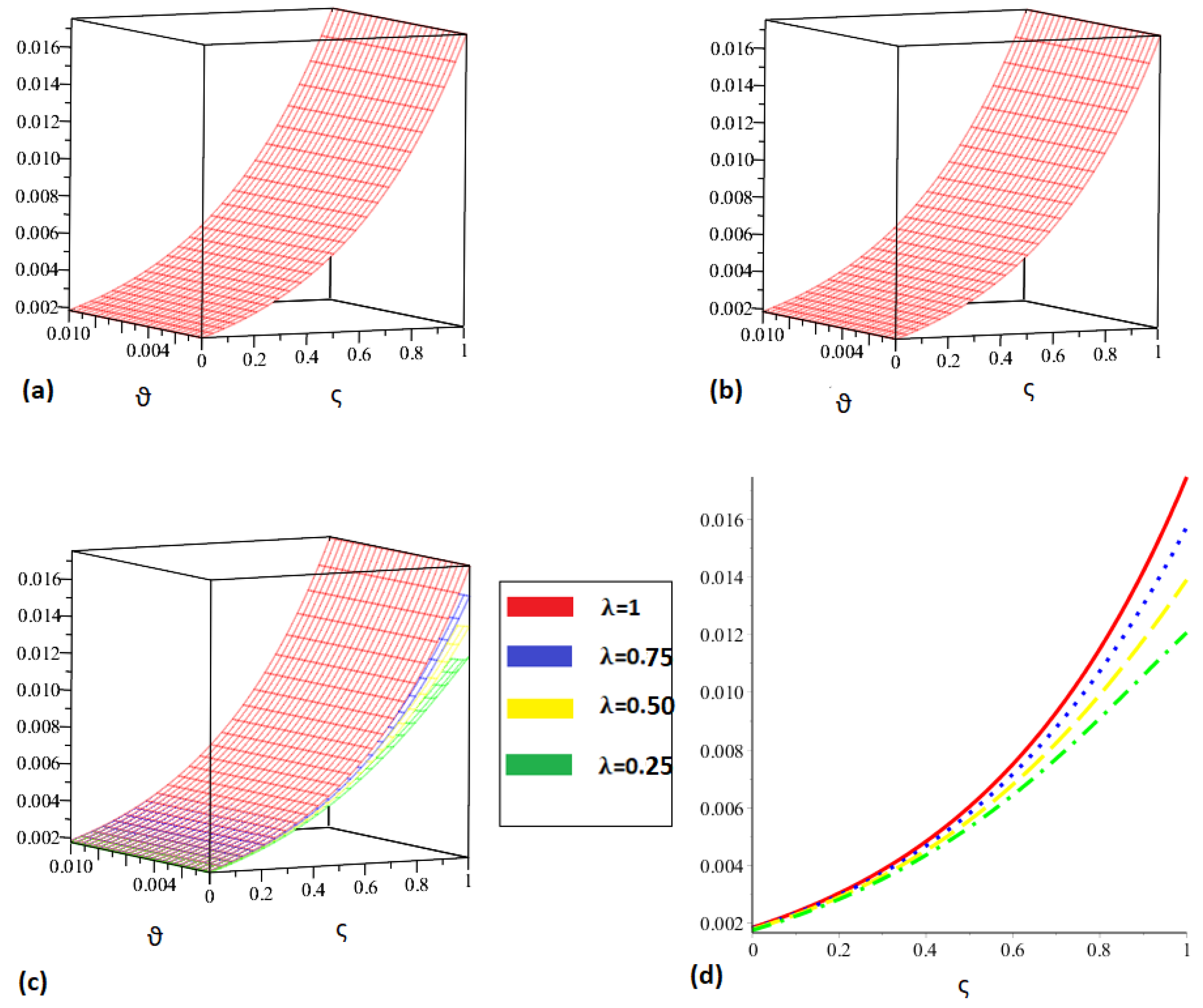
Figure 2.
Graphical representation of the accuracy of the solutions of Example 2 obtained using the proposed techniques and various fractional orders.
Figure 2.
Graphical representation of the accuracy of the solutions of Example 2 obtained using the proposed techniques and various fractional orders.

Table 1.
Numerical simulation of the accuracy of the solutions of Example 1 obtained using the proposed techniques for different orders of .
Table 1.
Numerical simulation of the accuracy of the solutions of Example 1 obtained using the proposed techniques for different orders of .
| (Approx) | (Exact) | |||||
|---|---|---|---|---|---|---|
| 0.2 | 0.002999 | 0.003012 | 0.003025 | 0.003037 | 0.003037 | |
| 0.4 | 0.004747 | 0.004776 | 0.004805 | 0.004835 | 0.004835 | |
| 0.01 | 0.6 | 0.007327 | 0.007392 | 0.007457 | 0.007524 | 0.007524 |
| 0.8 | 0.011097 | 0.011245 | 0.011392 | 0.011541 | 0.011541 | |
| 1 | 0.016543 | 0.016873 | 0.017203 | 0.017538 | 0.017538 | |
| 0.2 | 0.002999 | 0.003012 | 0.003024 | 0.003037 | 0.003037 | |
| 0.4 | 0.004746 | 0.004775 | 0.004805 | 0.004835 | 0.004835 | |
| 0.02 | 0.6 | 0.007324 | 0.007390 | 0.007456 | 0.007524 | 0.007524 |
| 0.8 | 0.011091 | 0.011240 | 0.011388 | 0.011541 | 0.011541 | |
| 1 | 0.016529 | 0.016863 | 0.017195 | 0.017538 | 0.017538 | |
| 0.2 | 0.002998 | 0.003011 | 0.003024 | 0.003037 | 0.003037 | |
| 0.4 | 0.004745 | 0.004775 | 0.004804 | 0.004835 | 0.004835 | |
| 0.03 | 0.6 | 0.007322 | 0.007388 | 0.007454 | 0.007524 | 0.007524 |
| 0.8 | 0.011086 | 0.011236 | 0.011384 | 0.011541 | 0.011541 | |
| 1 | 0.016517 | 0.016853 | 0.017187 | 0.017538 | 0.017538 | |
| 0.2 | 0.002998 | 0.003011 | 0.003024 | 0.003037 | 0.003037 | |
| 0.4 | 0.004744 | 0.004774 | 0.004803 | 0.004835 | 0.004835 | |
| 0.04 | 0.6 | 0.007319 | 0.007386 | 0.007453 | 0.007524 | 0.007524 |
| 0.8 | 0.011081 | 0.011231 | 0.011381 | 0.011541 | 0.011541 | |
| 1 | 0.016505 | 0.016843 | 0.017179 | 0.017538 | 0.017538 | |
| 0.2 | 0.002997 | 0.003010 | 0.003023 | 0.003037 | 0.003037 | |
| 0.4 | 0.004743 | 0.004773 | 0.004802 | 0.004835 | 0.004835 | |
| 0.05 | 0.6 | 0.004743 | 0.007384 | 0.007451 | 0.007524 | 0.007524 |
| 0.8 | 0.011076 | 0.011227 | 0.011377 | 0.011541 | 0.011541 | |
| 1 | 0.016494 | 0.016834 | 0.017171 | 0.017538 | 0.017538 |
Table 2.
Comparison between our solution and the solutions derived by the perturbation–iteration algorithm (PIA) and residual power series method (RPSM) at and for example 1 in terms of absolute error.
Table 2.
Comparison between our solution and the solutions derived by the perturbation–iteration algorithm (PIA) and residual power series method (RPSM) at and for example 1 in terms of absolute error.
| PIA Error | RPSM Error | Our Method Error | |||
|---|---|---|---|---|---|
| 0.2 | 0.1 | 0.1 | 3.85217 | 3.85217 | 3.8519486000 |
| 0.3 | 0.1 | 0.1 | 5.75911 | 5.75912 | 5.7583616000 |
| 0.4 | 0.1 | 0.1 | 7.65359 | 7.65352 | 7.6517330000 |
| 0.2 | 0.6 | 0.6 | 4.66337 | 4.66389 | 4.6473505000 |
| 0.3 | 0.6 | 0.6 | 6.86056 | 6.86314 | 6.8073230000 |
| 0.4 | 0.6 | 0.6 | 8.98263 | 8.99046 | 8.8581596000 |
| 0.2 | 0.9 | 0.9 | 5.12131 | 5.14241 | 4.9248718000 |
| 0.3 | 0.9 | 0.9 | 7.38186 | 7.48450 | 6.7502883000 |
| 0.4 | 0.9 | 0.9 | 9.57942 | 9.89139 | 8.1510249000 |
Table 3.
Numerical simulation of the accuracy of the solutions of Example 2 obtained using the proposed techniques for different orders of .
Table 3.
Numerical simulation of the accuracy of the solutions of Example 2 obtained using the proposed techniques for different orders of .
| (Approx) | (Exact) | |||||
|---|---|---|---|---|---|---|
| 0.2 | 0.030120 | 0.030147 | 0.030173 | 0.030197 | 0.030197 | |
| 0.4 | 0.035230 | 0.035259 | 0.035288 | 0.035315 | 0.035315 | |
| 0.01 | 0.6 | 0.040377 | 0.040410 | 0.040442 | 0.040473 | 0.040473 |
| 0.8 | 0.045568 | 0.045604 | 0.045641 | 0.045675 | 0.045675 | |
| 1 | 0.050807 | 0.050848 | 0.050889 | 0.050928 | 0.050928 | |
| 0.2 | 0.030119 | 0.030146 | 0.030172 | 0.030195 | 0.030195 | |
| 0.4 | 0.035229 | 0.035258 | 0.035288 | 0.035313 | 0.035313 | |
| 0.02 | 0.6 | 0.040376 | 0.040409 | 0.040441 | 0.040470 | 0.040470 |
| 0.8 | 0.045566 | 0.045603 | 0.045640 | 0.045672 | 0.045672 | |
| 1 | 0.050806 | 0.050847 | 0.050888 | 0.050925 | 0.050925 | |
| 0.2 | 0.030118 | 0.030145 | 0.030172 | 0.030192 | 0.030192 | |
| 0.4 | 0.035228 | 0.035257 | 0.035287 | 0.035310 | 0.035310 | |
| 0.03 | 0.6 | 0.040375 | 0.040408 | 0.040441 | 0.040467 | 0.040467 |
| 0.8 | 0.045565 | 0.045602 | 0.045639 | 0.045670 | 0.045670 | |
| 1 | 0.050804 | 0.050846 | 0.050887 | 0.050923 | 0.050923 | |
| 0.2 | 0.030117 | 0.030144 | 0.030171 | 0.030190 | 0.030190 | |
| 0.4 | 0.035227 | 0.035256 | 0.035286 | 0.035308 | 0.035308 | |
| 0.04 | 0.6 | 0.040374 | 0.040407 | 0.040440 | 0.040465 | 0.040465 |
| 0.8 | 0.045564 | 0.045601 | 0.045638 | 0.045667 | 0.045667 | |
| 1 | 0.050803 | 0.050845 | 0.050886 | 0.050920 | 0.050920 | |
| 0.2 | 0.030116 | 0.030144 | 0.030170 | 0.030187 | 0.030187 | |
| 0.4 | 0.035226 | 0.035256 | 0.035285 | 0.035305 | 0.035305 | |
| 0.05 | 0.6 | 0.040372 | 0.040406 | 0.040439 | 0.040462 | 0.040462 |
| 0.8 | 0.045563 | 0.045600 | 0.045637 | 0.045664 | 0.045664 | |
| 1 | 0.050802 | 0.050843 | 0.050885 | 0.050917 | 0.050917 |
Table 4.
Comparison between our solution and the solution derived by the variational iteration method (VIM) at and for example 2 in terms of absolute error.
Table 4.
Comparison between our solution and the solution derived by the variational iteration method (VIM) at and for example 2 in terms of absolute error.
| VIM Error | Our Method Error | |||
|---|---|---|---|---|
| 0.2 | 0.1 | 0.1 | 5.00091 | 4.9951950000 |
| 0.3 | 0.1 | 0.1 | 5.00091 | 7.4927920000 |
| 0.4 | 0.1 | 0.1 | 5.00091 | 9.9903860000 |
| 0.2 | 0.6 | 0.6 | 3.02003 | 5.0898600000 |
| 0.3 | 0.6 | 0.6 | 3.02003 | 7.6348000000 |
| 0.4 | 0.6 | 0.6 | 3.02003 | 1.0179720000 |
| 0.2 | 0.9 | 0.9 | 4.56780 | 5.2122800000 |
| 0.3 | 0.9 | 0.9 | 4.56780 | 7.8184000000 |
| 0.4 | 0.9 | 0.9 | 4.56780 | 1.0424500000 |
Disclaimer/Publisher’s Note: The statements, opinions and data contained in all publications are solely those of the individual author(s) and contributor(s) and not of MDPI and/or the editor(s). MDPI and/or the editor(s) disclaim responsibility for any injury to people or property resulting from any ideas, methods, instructions or products referred to in the content. |
© 2023 by the authors. Licensee MDPI, Basel, Switzerland. This article is an open access article distributed under the terms and conditions of the Creative Commons Attribution (CC BY) license (https://creativecommons.org/licenses/by/4.0/).
Share and Cite
MDPI and ACS Style
Ganie, A.H.; Mofarreh, F.; Khan, A. A Fractional Analysis of Zakharov–Kuznetsov Equations with the Liouville–Caputo Operator. Axioms 2023, 12, 609. https://doi.org/10.3390/axioms12060609
AMA Style
Ganie AH, Mofarreh F, Khan A. A Fractional Analysis of Zakharov–Kuznetsov Equations with the Liouville–Caputo Operator. Axioms. 2023; 12(6):609. https://doi.org/10.3390/axioms12060609
Chicago/Turabian StyleGanie, Abdul Hamid, Fatemah Mofarreh, and Adnan Khan. 2023. "A Fractional Analysis of Zakharov–Kuznetsov Equations with the Liouville–Caputo Operator" Axioms 12, no. 6: 609. https://doi.org/10.3390/axioms12060609
Note that from the first issue of 2016, this journal uses article numbers instead of page numbers. See further details here.