
Iterative Stability Analysis for Generalized α-Nonexpensive Mappings with Fixed Points

1
Department of Mathematical Sciences, Fatima Jinnah Women University, Rawalpindi 46000, Pakistan
2
Department of Mathematical and Statistics, International Islamic University, Islamabad 44000, Pakistan
3
Department of Mathematical and Statistical Sciences, University of Alberta, Edmonton, AB T6G 2G1, Canada
4
Department of Mathematics, King Abdulaziz University, P.O. Box 80203, Jeddah 21589, Saudi Arabia
*
Author to whom correspondence should be addressed.
Axioms 2024, 13(3), 156; https://doi.org/10.3390/axioms13030156
Submission received: 2 January 2024
/
Revised: 19 February 2024
/
Accepted: 21 February 2024
/
Published: 27 February 2024
(This article belongs to the Special Issue Research on Fixed Point Theory and Application)
Abstract
:This article introduces a novel iterative process, denoted as , designed for the class of generalized -Nonexpensive mappings. The study establishes strong and weak convergence theorems within the context of Banach spaces, supported by carefully chosen assumptions. The convergence results contribute to the theoretical foundation of iterative processes in functional analysis. The presented framework is applied to address nonlinear integral equations, showcasing the versatility and applicability of the proposed for the class of generalized iteration process. Additionally, the article includes numerical examples that not only validate the theoretical findings but also provide insights into the practical utility of the developed methodology.
1. Introduction
When the presence of a solution for a given operator is affirmed, ordinary analytical approaches often fall short of obtaining such solutions. To surmount this challenge, resorting to approximation methods becomes imperative. One of the key findings in fixed point (FP) theory is the Banach contraction theorem, which Polish mathematician Stefan Banach presented in 1922 [1]. The Banach contraction theorem relies on the convergence of a fundamental iterative process known as the sequence of successive approximations or the Picard iteration process. This theorem addresses an FP problem for a contraction mapping defined on a complete metric space [2]. It has evolved into a crucial tool for demonstrating the existence and approximation of solutions to nonlinear functional equations, including those arising in differential, integral, and partial differential equations. While certain scenarios ensure the existence of a solution to the FP problem, determining the exact solution may be infeasible. In these situations, there is a great desire to approximate the solution to the given problem, which prompts the creation of numerous iterative procedures. In the domain of nonexpansive mappings, denoted as NonExp mappings, the assurance of Picard iteration process convergence to a FP is not guaranteed for specific classes of NonExp mappings [2]. Consequently, alternative iterative approaches are employed, incorporating different procedural steps and parameter sets. Several iterative processes, such as those introduced by Mann [3], Ishikawa [4], Noor [5], S iteration by Agarwal et al. [6], Abbas [7], and Picard-S [8], have undergone extensive investigation.
In 2018, Ullah and Arshad [9] introduced the M iterative scheme for Suzuki mappings, showcasing its faster convergence compared to the aforementioned processes. In 2008, Suzuki [10] proved analogous FP theorems in Banach space, denoted as (BS), showing that the class of maps meeting condition (C) is weaker than the idea of NonExp mappings. Browder in 1965 [11] focused on uniformly convex BS, while Kirk [12], in a reflexive BS, established FPs for NonExp mappings. More recently, Ullah et al. [13] applied the M iteration scheme to find FPs of generalized -Nonexpensive mappings, denoted as GNZ--NonExp mappings, in BS.
In 2020, Ali and Ali [14] introduced a novel iteration process, the F iterative process, for generalized contractions. They demonstrated the stability and superior convergence rate of this F iterative scheme compared to other iteration processes in the context of generalized contractions.
In 2021, Junaid et al. [2] established a connection between the F iteration process and the class of GNZ--NonExp mappings. Under suitable assumptions, they derived both strong and weak convergence outcomes within the framework of BS. The following iteration process (1) for uniformly convex Banach space, denoted as UCBS, as given in [2], is described as follows:
where is GNZ--NonExp mapping and .
In this paper, we modify the iterative process given in [2] for GNZ--NonExp mappings. For this purpose a new function is defined in the above iterative process (1). By using this new function, we observe early convergence with high accuracy. This finding is supported by providing two different examples. The obtained numerical results are presented in Table 1 and Table 2. These results are compared with the previous iterative processes. Another interesting property of the above process is that if the number of functions similar to is increased, then rapid convergence along with high accuracy can be obtained. However, for simplicity, we consider only one function in our study.
In this manuscript, we have six sections. Section 1, includes the introduction of our research, and Section 2 is related to the preliminaries and results, which are helpful to construct the main result of the paper. Section 3 is the main part of the paper where we define our main scheme and the strong and weak convergence results of the scheme, whereas Section 4 and Section 5 are about the useability of our results. Here, we apply our findings for the solution of non-linear integral equation. In the last section, we conclude our findings.
2. Preliminaries
This section deals with the preliminaries and results, which help construct the main results of this article.
Definition 1
([2]). Suppose that is a BS and is a nonempty subset. Let be a mapping. Then Ω is said to be
- 1.
- NonExp if , for all ;
- 2.
- endowed with condition (C) if for all with.
Definition 2
([2]). Suppose that is a BS and is a nonempty subset. Let be a mapping. Then Ω is said to be GNZ-α-NonExp if for all with
⇒
for some .
Definition 3
([15]). A BS is said to satisfy the Opial condition (OpCd), if for every sequence that weakly converges to , the following condition holds:
Definition 4
([2]). Suppose that is a BS and is nonempty and is a bounded sequence. For a fix the following assumptions hold:
- 1.
- at the point j of asymptotic radius of bounded sequence by
- 2.
- the connection of with asymptotic radius of bounded sequence by
- 3.
- the connection of asymptotic center of bounded sequence with by
Pant and Shukla [17] described the following facts about GNZ--NonExp mappings.
Proposition 1
([17]). For a BS with a closed, nonempty subset , and a mapping with , the following statements hold:
- 1.
- If Ω satisfies condition (C), it is considered a GNZ-α-NonExp mapping.
- 2.
- If Ω is a GNZ-α-NonExp mapping with a nonempty FP, then for any and as the FP of Ω, .
- 3.
- When Ω is a GNZ-α-NonExp mapping, the set is closed. Additionally, if the fundamental space is strictly convex and is convex, then is convex.
- 4.
- For all , if Ω is a GNZ-α-NonExp mapping, the inequality holds:
- 5.
- If the fundamental space satisfies the OpCd, then Ω is a GNZ-α-NonExp mapping. Moreover, if weakly converges to and , then .
We have an interesting property of a UCBS [18].
Lemma 1
3. Generalized Iterative Scheme for -NonExp Mappings
Suppose that is a UCBS and is a GNZ--NonExp mapping. Then a modified iteration process for the present study is described as
where is GNZ--NonExp mapping and .
In the mentioned procedure, a novel function is introduced. It is noted that attaining early convergence with enhanced accuracy is possible by augmenting the number of functions akin to utilized in the aforementioned approach. However, for the sake of simplicity in the current scenario, we focus on a single function . We term this innovative iterative method as , representing a generalized version of the scheme proposed by Junaid [2].
In this section, the results related to the strong and weak convergence for the new iterative scheme are described.
Lemma 2.
Suppose that is any UCBS and is closed, nonempty and convex. Let be a GNZ-α-NonExp mapping satisfying and be a sequence of iterates (2). Then always exists for every .
Proof.
Suppose . Using Proposition 1(2), we have
Consequently,
which means that is bounded as well as non-increasing. It follows that , exists for each . □
We now provide the necessary and sufficient requirements for the existence of FP for any GNZ--NonExp mapping in UCBS.
Theorem 1.
Consider any UCBS, where is the space, and is a closed, nonempty, and convex subset. Assume that is a GNZ-α-NonExp mapping, and represents a sequence of iterates (2). Then if and only if is bounded and .
Proof.
Assuming and , for any , utilizing Lemma 1, we observe that exists and is bounded. Let us denote this limit as , i.e.,
From Lemma 1, we have
By applying the lim and using (4), we have
Since is in the set , and by using Proposition 1(2), we get the following:
From Lemma 1, we have
Thus,
By Lemma 1, we get
Conversely, we will demonstrate the non-emptiness of the set under the conditions that is bounded and approaches zero as . If we apply the Proposition 1(4), we have
We observe that . In the case of UCBS, the set has cardinality equal to one. This concludes that . Thus, the set is nonempty. □
The weak and strong convergences of iteration (2) are established as follows.
Theorem 2.
Consider any UCBS satisfying the OpCd, where is a closed, nonempty, and convex subset. If is a GNZ-α-NonExp mapping with , and represents a sequence of iterates (2), then weakly converges to a FP of Ω.
Proof.
By Theorem 1, is bounded in . Since is a UCBS, will be reflexive; hence, the bounded sequence admits a weakly convergent sub sequence with weak limit, namely, . If we apply Theorem 1 on this subsequence, we obtain . Thus, by Proposition 1(5), one has . If we prove that is a weak limit for , then the proof will be finished. We prove this by contradiction. Suppose is not a weak limit for ; that is, another subsequence of exists that admits a weak limit . The same calculations give . Now we know that admits the OpCd. Thus, one has
The above estimate suggests a contradiction and, hence, we must accept that . Accordingly, converges weakly to . □
Theorem 3.
Assuming that is a UCBS satisfying the OpCd, and is a convex, nonempty, and compact subset. If is a GNZ-α-NonExp mapping with , and denotes a sequence of iterates (2), then exhibits strong convergence to a FP of Ω.
Proof.
Due to the convexity of , we have . Accordingly, we have a subsequence of with for some . On the other hand, using Theorem 1, . Thus, by Proposition 1(4), one has
Hence, if we let , then . Hence, is a FP of , and by Lemma 2, exists. Accordingly, is also a strong limit of . □
Theorem 4.
Assuming is a UCBS equipped with the OpCd, and is a closed, nonempty, and convex subset. If is a GNZ-α-NonExp mapping with , and represents a sequence of iterates (2) such that , then strongly converges to an FP of Ω.
Proof.
According to Lemma 2, the limit exists for every FP of . Consequently, also exists, and
The above limit provides us two subsequences and of and , respectively, in the following way
By Lemma 2, we see that is non increasing and so
It follows that if , then
Consequently, we obtain that , which shows that is a Cauchy sequence in and so it converges to an element . By Proposition 1(3), is closed and so . By Lemma 2, exists and, hence, is the strong limit of . □
Theorem 5.
Assume that is a UCBS with the OpCd, and is a closed, nonempty, and convex subset. Let be a mapping satisfying condition (C), with and representing a sequence of iterates (2). Then, exhibits strong convergence to a FP of Ω.
Proof.
From (1), we have
By using the definition of condition (I) [2], we have
It follows that
By Theorem 4, is strongly convergent to an FP of . □
To support the main results, we provide two examples by Proposition 1(1) of GNZ--NonExp mapping, which is provided with C. By using these examples, we implement our new proposed method to obtain numerical results. These results are compared with other iteration schemes that are used for GNZ--NonExp mappings.
Example 1.
Consider the closed and bounded subset of the real number space . Define as
Our aim is to establish that Ω is a GNZ-α-NonExp mapping with , while it does not fall under the category of Suzuki mappings. This example, therefore, extends beyond the class of Suzuki mappings.
Case I: If , then we have
Case II: If , then we have
Case III: If and , then we have
So
for all .
Example 2.
Consider the closed and bounded subset within the Banach space . Let be defined as
In this example, we prove again that Ω is a GNZ-α-NonExp mapping with , but not a Suzuki mapping. This example thus exceeds the class of Suzuki mappings.
Case I: If , then we have
Case II: If , then we have
Case III: If and , then we have
So,
for all .
We will now assess the efficiency of the proposed iteration scheme in comparison to other prominent schemes, namely F [2], M [9], Noor [5], S [6], Picard-S [8], Picard [1], Ishikawa [4], and Mann [3], within the broader context of GNZ--NonExp mappings. Each of these schemes exhibits distinct convergence rates for GNZ--NonExp mappings. Upon comparing these leading schemes, it becomes evident that F [2], M [9], and S [6] demonstrate a higher rate of convergence when compared to Noor [5], Picard-S [8], Picard [1], Ishikawa [4], and Mann [3]. Essentially, the former set of schemes proves to be more efficient for contractions and NonExp mappings. The effectiveness of is clearly observed in Table 1 and Table 2, which provide results for GNZ--NonExp mappings as presented in Examples 1 and 2. Additionally, Figure 1 offers insights into the performance of these leading schemes. It is evident that the iterative scheme surpasses the other schemes in the general context of GNZ--NonExp mappings.
4. Application to Nonlinear Integral Equation
In this section, we explore the application of our findings to a nonlinear integral equation of the form
where , , and are continuous functions. Let denote the space of all continuous functions defined on , and the order relations ≤ in are defined as follows: For , for all . Define by
Theorem 6.
Consider the space representing all continuous real-valued functions defined on . Let be the mapping defined as
where , , and are continuous functions. Additionally, suppose the following conditions are met:
- 1.
- There exists a continuous mapping such thatfor all and .
- 2.
- There exists such that
Then the integral Equation (4) possesses a solution.
Proof.
Suppose . If
for all , then
Thus, we
Thus, we have
and
for all and .
Clearly, satisfies the condition (C) and by Definition 2, is a GNZ--NonExp mapping. All the conditions given in Theorem 5 are satisfied. Thus, has an FP that is the solution of the nonlinear integral Equation (4). □
5. Experimental Results
We have a nonlinear integral equation of the form
The equation represents a relationship between the derivative of an unknown function and the integral of a function over a given interval , weighted by the kernel function . The function represents a driving force.
To solve this equation, we will employ the FP Iteration method. We start with an initial approximation and update it iteratively by using the following formula:
where n represents the iteration number.
In the example, we will consider specific functions for , , and , and the interval . We will solve (9) by using the FP Iteration method with an initial approximation . We will evaluate the solution at various points within the interval .
Table 3 provided in the example shows the approximation, exact value, and error at each iteration. Each row corresponds to a specific iteration, with the approximation denoted as , the exact value denoted as , and the calculated error being the absolute difference between the approximation and the exact value .
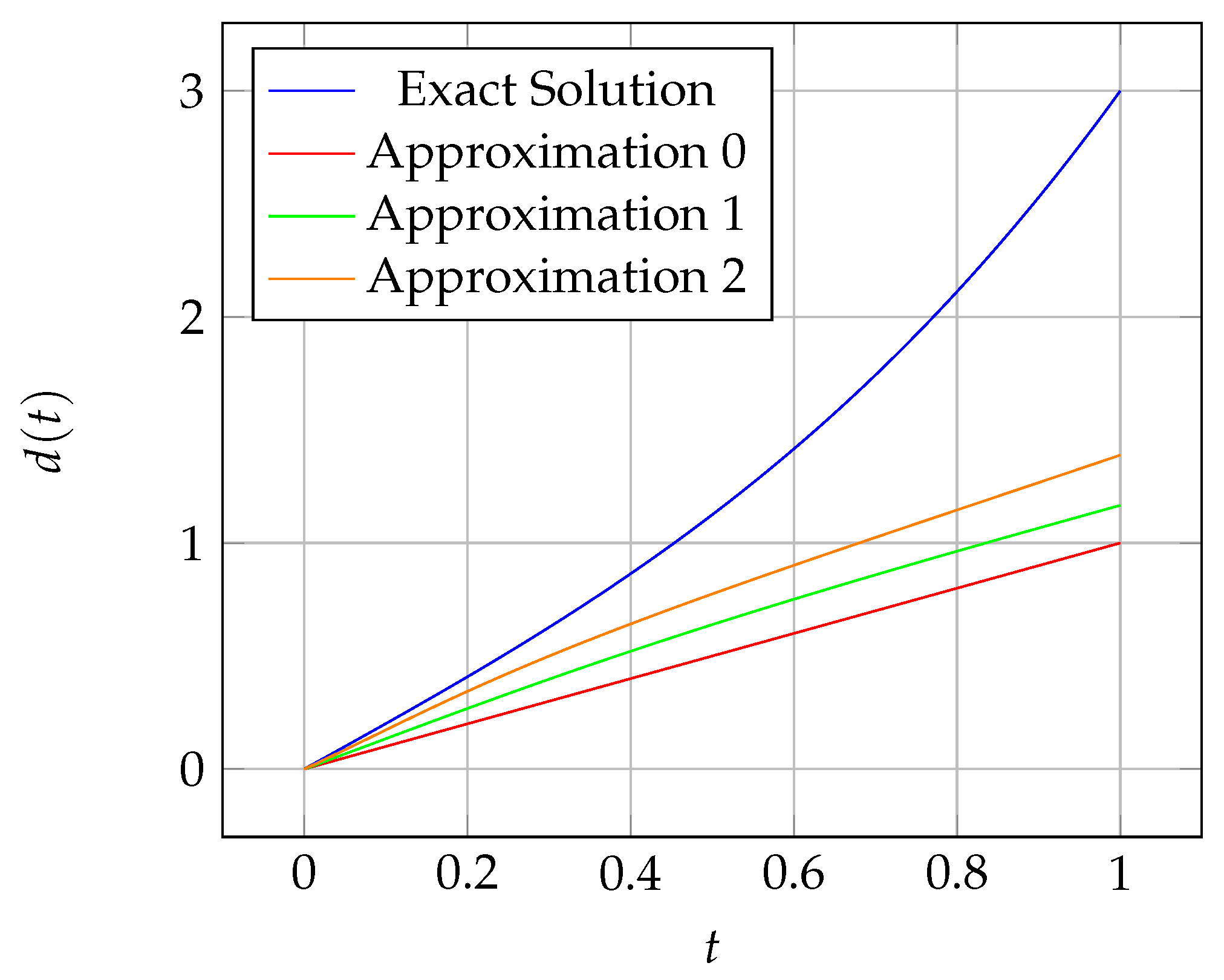
Furthermore, a graphical representation will be given to visualize the convergence behavior of the iterative scheme. The graph will show the exact solution and the iteratively computed approximations for each iteration.
Overall, the example will demonstrate the process of solving a nonlinear integral equation by using the FP Iteration method and provide insights into the convergence behavior through the table and graph.
Example 3.
Consider the following nonlinear integral equation:
where and are continuous functions, and is a kernel function. To solve (10), we can use an iterative scheme called the FP Iteration method. We start with an initial approximation and iteratively update it by using the following formula:
where n represents the iteration number.
Now, we assume the following specific functions for our example:
and the interval as .
We will solve (10) by using the FP Iteration method with an initial approximation . We will evaluate the solution at various points in the interval . Table 3 shows the approximation, exact value, and error at each iteration while Table 4 shows the solution function and the iteratively computed approximations for each iteration.
6. Conclusions
This paper presents several novel contributions:
- (i)
- We introduce a new iterative scheme, denoted as , specifically designed for GNZ--NonExp mappings. Our findings indicate that the inclusion of an additional function facilitates rapid convergence for -NonExp mappings. We establish both weak and strong convergence for the modified iterative scheme.
- (ii)
- (iii)
- We provide diverse examples to illustrate and support our findings, showcasing the efficiency of the proposed algorithm across various iterative algorithms in the existing literature. This is achieved through different parameter choices and initial guesses.
- (iv)
- Consequently, our results extend the core findings of Ahmad et al. [2], serving as generalizations and refinements of the outcomes presented by Ali and Ali [14] and Ahmad et al. [2]. We extend our results from contraction to NonExp mappings and GNZ--NonExp mappings, emphasizing enhanced convergence speed.
- (v)
- To demonstrate the practical applicability of our results, we apply our findings to ascertain solutions for nonlinear integral equations.
Author Contributions
Conceptualization, M.I. and A.A.; methodology, M.I. and A.A. software, M.I.; validation, A.A., H.A.S. and A.H.; formal analysis, A.A.; investigation, H.A.S.; resources, A.H.; data curation, A.A.; writing—original draft preparation, M.I.; writing—review and editing, A.A.; visualization, A.A.; supervision, H.A.S.; project administration, A.H.; funding acquisition, H.A.S. and A.H. Authors equally conceived of the study, participated in its design and coordination, drafted the manuscript, and participated in the sequence alignment, and read and approve the final manuscript. All authors have read and agreed to the published version of the manuscript.
Funding
The authors declare that there is no funding available for this paper.
Informed Consent Statement
We would like to mention that this article does not contain any studies with animals and does not involve any studies on human beings.
Data Availability Statement
Not applicable.
Acknowledgments
For the financial support and encouagment the authors are thankfull to the employ of King Abdulaziz University, P. O . Box 80203, Jeddah 21589, Saudi Arabia.
Conflicts of Interest
The authors declare that they have no competing interests.
References
- Banach, S. Sur les operations dans les ensembles abstraits et leur application aux equations integrals. Fund. Math. 1922, 3, 133–181. [Google Scholar] [CrossRef]
- Ahmad, J.; Ullah, K.; Arshad, M.; de la Sen, M. Iterative approximation of fixed points by using F iteration Process in Banach spaces. J. Funct. Spaces 2021, 2021, 6994660. [Google Scholar] [CrossRef]
- Mann, W.R. Value methods in iteration. Proc. Am. Math. Soc. 1953, 4, 506–510. [Google Scholar] [CrossRef]
- Ishikawa, S. Points by a new iteration method. Proc. Am. Math. Soc. 1974, 4, 147–150. [Google Scholar] [CrossRef]
- Noor, M.A. New approximation schemes for genreral variational inequalities. J. Math. Anal. Appl. 2000, 251, 217–229. [Google Scholar] [CrossRef]
- Agarwal, R.P.; O’Regan, D.; Sahu, D.R. Fixed Point Theory for Lipschitzian-Type Mappings with Applications; Springer: New York, NY, USA, 2009. [Google Scholar]
- Abbas, M.; Nazir, T. A new faster iteration process applied to constrained minimization and feasibility problems. Mat. Vesnik 2014, 66, 223–234. [Google Scholar]
- Khan, S.H. A Picard-Mann hybrid iterative process. Fixed Point Theory Appl. 2013, 2013, 69. [Google Scholar] [CrossRef]
- Ullah, K.; Arshad, M. Numerical reckoning fixed points for Suzuki’s generalized non expansive mappings via new iteration process. Filomat 2018, 32, 187–196. [Google Scholar] [CrossRef]
- Suzuki, T. Fixed point theorems and convergence theorems for some generalized nonexpensive mappings. J. Math. Anal. Appl. 2008, 340, 1088–1095. [Google Scholar] [CrossRef]
- Browder, F.E. Non expansive nonlinear operators in a Banach space. Proc. Natl. Acad. Sci. USA 1965, 54, 1041–1044. [Google Scholar] [CrossRef] [PubMed]
- Kirk, W.A. A fixed point theorem for mappings which do not increase distances. Am. Math. Mon. 1965, 72, 1004–1006. [Google Scholar] [CrossRef]
- Ullah, K.; Ayaz, F.; Ahmed, J. Some convergence results of M iterative process in Banach spaces. Asian-Eur. J. Math. 2021, 41, 2150017. [Google Scholar] [CrossRef]
- Ali, F.; Ali, J. A new iterative scheme to approximating fixed points and the solution of a delay differential equation. J. Nonlinear Convex Anal. 2020, 21, 2151–2163. [Google Scholar]
- Opial, Z. Weak convergence of the sequence of successive approximation for non expansive mappings. Bull. Aust. Math. Soc. 1967, 73, 591–598. [Google Scholar] [CrossRef]
- Agarwal, R.P.; O’Regan, D.; Sahu, D.R. Iterative construction of fixed points of nearly asymtotically non-expensive mappings. J. Nonlinear Convex Anal. 2007, 8, 61–79. [Google Scholar]
- Paint, R.; Shukla, R. Approximating fixed points of generalized α-non expansive mappings in Banach spaces. Numer. Funct. Anal. Optim. 2017, 38, 248–266. [Google Scholar] [CrossRef]
- Schu, J. Weak and strong convergence to fixed points of asymptotically non expansive mappings. Bull. Aust. Math. Soc. 1991, 43, 153–159. [Google Scholar] [CrossRef]
Figure 1.
Graphical representation of convergence analysis for the GNZ--NonExp mappings given in Examples 1 and 2 with other schemes.
Figure 1.
Graphical representation of convergence analysis for the GNZ--NonExp mappings given in Examples 1 and 2 with other schemes.

Figure 2.
Graphical representation of the approximation and exact values given in Table 3.
Figure 2.
Graphical representation of the approximation and exact values given in Table 3.
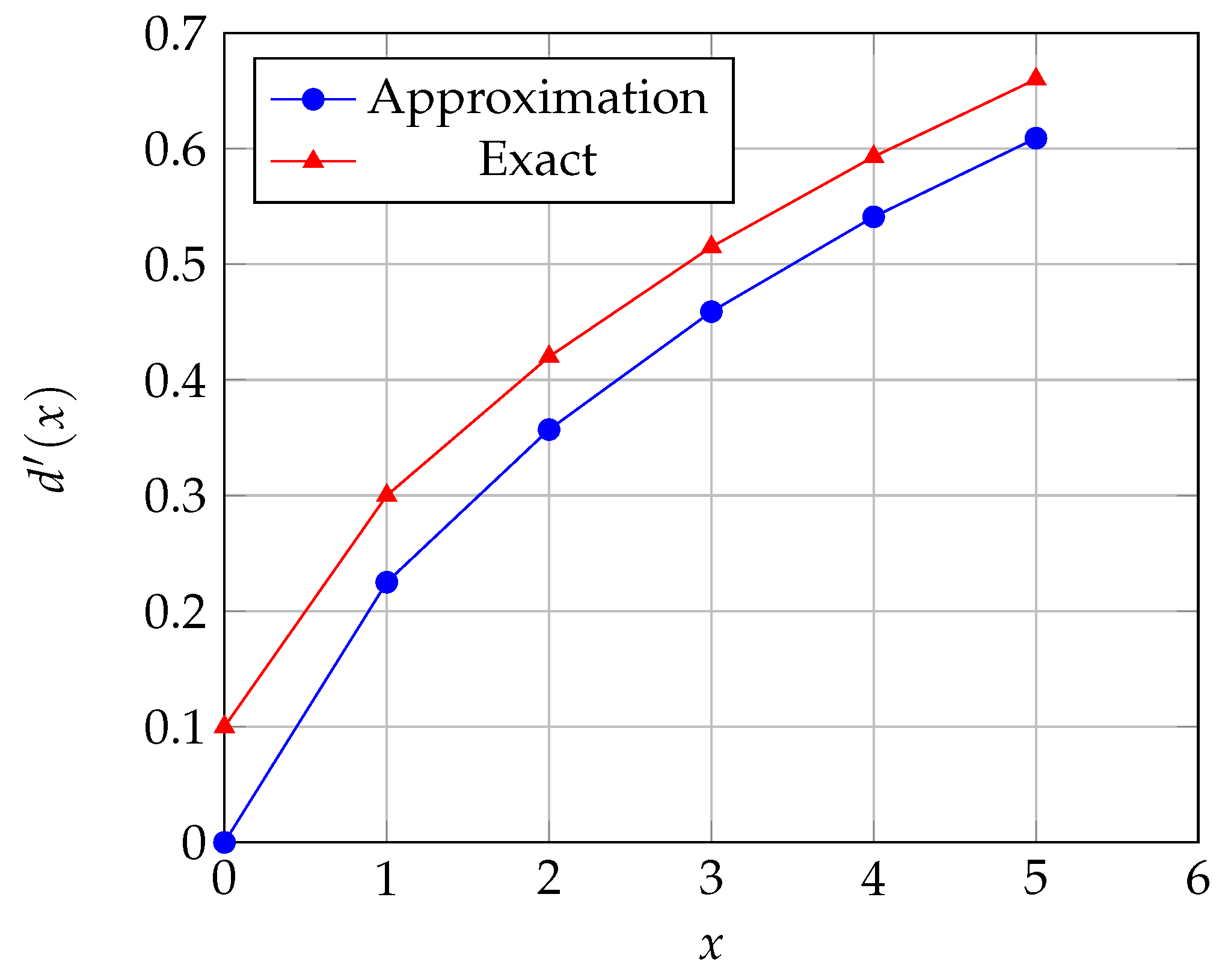
Figure 3.
Graphical representation of the solution function and the iteratively computed approximations for each iteration.
Figure 3.
Graphical representation of the solution function and the iteratively computed approximations for each iteration.

Table 1.
Convergence comparison of scheme (2) for GNZ--NonExp mapping given in Example 1 with other schemes with respect to the number of iterations.
Table 1.
Convergence comparison of scheme (2) for GNZ--NonExp mapping given in Example 1 with other schemes with respect to the number of iterations.
| N | F [2] | M [9] | S [6] | Picard-S [8] | Ishikawa [4] | Mann [3] | |
|---|---|---|---|---|---|---|---|
| 1 | 7.9 | 7.9 | 7.9 | 7.9 | 7.9 | 7.9 | 7.9 |
| 2 | 7.042188 | 7.06468750 | 7.12937500 | 7.3256875 | 7.1628437 | 7.3931875 | 7.51750000 |
| 3 | 7.001978 | 7.00464941 | 7.01859766 | 7.11785816 | 7.02946454 | 7.17177379 | 7.29756250 |
| 4 | 7.000093 | 7.00033418 | 7.00267341 | 7.04264992 | 7.00533124 | 7.07504367 | 7.17109844 |
| 5 | 7.000004 | 7.00002402 | 7.00038430 | 7.01543394 | 7.00096462 | 7.03278471 | 7.09838160 |
| 6 | 7 | 7.00000173 | 7.00005524 | 7.00558516 | 7.00017454 | 7.01432282 | 7.05656942 |
| 7 | 7 | 7.00000012 | 7.00000794 | 7.00202113 | 7.00003158 | 7.00625728 | 7.0325 2742 |
| 8 | 7 | 7.00000001 | 7.00000114 | 7.0007314 | 7.00000571 | 7.00273365 | 7.01870 326 |
| 9 | 7 | 7 | 7.00000016 | 7.00026467 | 7.00000103 | 7.00119426 | 7.0107543 8 |
| 10 | 7 | 7 | 7.00000002 | 7.00009578 | 7.00000019 | 7.00052174 | 7.00618377 |
| 11 | 7 | 7 | 7 | 7.00000003 | 7.00003466 | 7.00022794 | 7.00355567 |
| 12 | 7 | 7 | 7 | 7.00001254 | 7.00000001 | 7.00009959 | 7.00204451 |
| 13 | 7 | 7 | 7 | 7.00000454 | 7 | 7.00004350 | 7.00117559 |
| 14 | 7 | 7 | 7 | 7.00000164 | 7 | 7.00001901 | 7.00067597 |
| 15 | 7 | 7 | 7 | 7.00000059 | 7 | 7.00000830 | 7.00038868 |
| 16 | 7 | 7 | 7 | 7.00000022 | 7 | 7.00000363 | 7.00022349 |
| 17 | 7 | 7 | 7 | 7.00000008 | 7 | 7.00000158 | 7.00012851 |
| 18 | 7 | 7 | 7 | 7.00000003 | 7 | 7.00000069 | 7.00007389 |
| 19 | 7 | 7 | 7 | 7.00000001 | 7 | 7.00000030 | 7.00004249 |
| 20 | 7 | 7 | 7 | 7 | 7 | 7.00000013 | 7.00002443 |
| 21 | 7 | 7 | 7 | 7 | 7 | 7.00000006 | 7.00001405 |
| 22 | 7 | 7 | 7 | 7 | 7 | 7.00000003 | 7.00000808 |
| 23 | 7 | 7 | 7 | 7 | 7 | 7.00000001 | 7.00000464 |
| 24 | 7 | 7 | 7 | 7 | 7 | 7 | 7.00000260 |
Table 2.
Convergence comparison of scheme (2) for GNZ--NonExp mapping given in Example 2 with other schemes with respect to the number of iterations.
Table 2.
Convergence comparison of scheme (2) for GNZ--NonExp mapping given in Example 2 with other schemes with respect to the number of iterations.
| N | F [2] | Picard [1] | Mann [3] | Ishikawa [4] | M [9] | Noor [5] | |
|---|---|---|---|---|---|---|---|
| 1 | 6.9 | 6.9 | 6.9 | 6.9 | 6.9 | 6.9 | 6.9 |
| 2 | 6.04921875 | 6.0984387 | 6.45 | 6.7875 | 6.773438 | 6.172266 | 6.77168 |
| 3 | 6.002692 | 6.010767 | 6.225 | 6.689063 | 6.664673 | 6.032973 | 6.661655 |
| 4 | 6.000147 | 6.001178 | 6.1125 | 6.60293 | 6.571203 | 6.006311 | 6.567318 |
| 5 | 6.000008 | 6.000129 | 6.05625 | 6.527563 | 6.490878 | 6.001208 | 6.48643 |
| 6 | 6 | 6.000014 | 6.028125 | 6.461618 | 6.421848 | 6.000231 | 6.417076 |
| 7 | 6 | 6.000002 | 6.014063 | 6.403916 | 6.362526 | 6.000044 | 6.35761 |
| 8 | 6 | 6 | 6.007031 | 6.353426 | 6.311546 | 6.0000088 | 6.306623 |
| 9 | 6 | 6 | 6.003516 | 6.309248 | 6.267734 | 6.000002 | 6.262905 |
| 10 | 6 | 6 | 6.001758 | 6.270592 | 6.230084 | 6 | 6.225421 |
| 11 | 6 | 6 | 6.000879 | 6.236768 | 6.197729 | 6 | 6.193281 |
| 12 | 6 | 6 | 6.000439 | 6.207172 | 6.169923 | 6 | 6.165723 |
| 13 | 6 | 6 | 6.00022 | 6.181276 | 6.146028 | 6 | 6.142094 |
| 14 | 6 | 6 | 6.00011 | 6.158616 | 6.125493 | 6 | 6.121835 |
| 15 | 6 | 6 | 6.000055 | 6.138789 | 6.107845 | 6 | 6.104464 |
| 16 | 6 | 6 | 6.000027 | 6.12144 | 6.092679 | 6 | 6.08957 |
| 17 | 6 | 6 | 6.000014 | 6.10626 | 6.079646 | 6 | 6.076799 |
| 18 | 6 | 6 | 6.000007 | 6.092978 | 6.068446 | 6 | 6.065849 |
| 19 | 6 | 6 | 6.000003 | 6.081356 | 6.058821 | 6 | 6.05646 |
| 20 | 6 | 6 | 6.000002 | 6.0711867 | 6.050549 | 6 | 6.04841 |
| 21 | 6 | 6 | 6.000001 | 6.062288 | 6.043441 | 6 | 6.041508 |
| 22 | 6 | 6 | 6 | 6.0545027 | 6.037332 | 6 | 6.03559 |
| 23 | 6 | 6 | 6 | 6.047689 | 6.027571 | 6 | 6.030516 |
| 24 | 6 | 6 | 6 | 6.041728 | 6.023693 | 6 | 6.026165 |
Table 3.
Approximation, exact, and error values for different iterations.
| Iteration | Approximation | Exact | Error |
|---|---|---|---|
| 0 | 0.000 | 0.100 | - |
| 1 | 0.225 | 0.300 | 0.075 |
| 2 | 0.357 | 0.420 | 0.063 |
| 3 | 0.459 | 0.515 | 0.056 |
| 4 | 0.541 | 0.593 | 0.052 |
| 5 | 0.609 | 0.660 | 0.051 |
Table 4.
Solution function and the iteratively computed approximations for different iterations.
| Iteration | Approximation | Exact | Error |
|---|---|---|---|
| 0 | |||
| 1 | |||
| 2 | |||
| … | … | … | … |
Disclaimer/Publisher’s Note: The statements, opinions and data contained in all publications are solely those of the individual author(s) and contributor(s) and not of MDPI and/or the editor(s). MDPI and/or the editor(s) disclaim responsibility for any injury to people or property resulting from any ideas, methods, instructions or products referred to in the content. |
© 2024 by the authors. Licensee MDPI, Basel, Switzerland. This article is an open access article distributed under the terms and conditions of the Creative Commons Attribution (CC BY) license (https://creativecommons.org/licenses/by/4.0/).
Share and Cite
MDPI and ACS Style
Iqbal, M.; Ali, A.; Sulami, H.A.; Hussain, A. Iterative Stability Analysis for Generalized α-Nonexpensive Mappings with Fixed Points. Axioms 2024, 13, 156. https://doi.org/10.3390/axioms13030156
AMA Style
Iqbal M, Ali A, Sulami HA, Hussain A. Iterative Stability Analysis for Generalized α-Nonexpensive Mappings with Fixed Points. Axioms. 2024; 13(3):156. https://doi.org/10.3390/axioms13030156
Chicago/Turabian StyleIqbal, Maryam, Amjad Ali, Hamid Al Sulami, and Aftab Hussain. 2024. "Iterative Stability Analysis for Generalized α-Nonexpensive Mappings with Fixed Points" Axioms 13, no. 3: 156. https://doi.org/10.3390/axioms13030156
Note that from the first issue of 2016, this journal uses article numbers instead of page numbers. See further details here.