Estimation of Gumbel Distribution Based on Ordered Maximum Ranked Set Sampling with Unequal Samples

Abstract

Sample selection is one of the most important factors in estimating the unknown parameters of distributions, as it saves time, saves effort, and gives the best results. One of the challenges is deciding on a suitable distribution estimate technique and adequate sample selection to provide the best results in comparison with earlier research. The method of moments (MOM) was decided on to estimate the unknown parameters of the Gumbel distribution, but with four changes in the sample selection, which were simple random sample (SRS), ranked set sampling (RSS), maximum ranked set sampling (MRSS), and ordered maximum ranked set sampling (OMRSS) techniques, due to small sample sizes. The MOM is a traditional method for estimation, but it is difficult to use when dealing with RSS modification. RSS modification techniques were used to improve the efficiency of the estimators based on a small sample size compared with the usual SRS estimator. A Monte Carlo simulation study was carried out to compare the estimates based on different sampling. Finally, two datasets were used to demonstrate the adaptability of the Gumbel distribution based on the different sampling techniques.

1. Introduction

McIntyre [1] initially offered the idea of using ranked set sampling (RSS) to estimate average pasture and forage yields, and subsequent discussions by Takahasi and Wakimoto [2] elaborated on this strategy. Recently, it has been used for issues in domains including environmental research, reliability engineering, and quality assurance when measuring the variable of interest might be prohibitively costly. When compared with simple random sampling (SRS), RSS may increase the efficiency and accuracy while decreasing costs. For instance, Lavine [3] investigated a comparison of RSS and SRS within a Bayesian framework. The literature has grown considerably in recent years, with most of it being summed up within a monograph by Chen et al. [4]. The RSS scheme can be described as follows: First, select an SRS of n sets of size n from the target population. Second, select the element of rank i from the ith set in a cycle for $\{i=1,2,\dots ,n\}$. The process can be repeated m times to obtain an RSS sample of size $nm$. Let $\{X_1,X_2,\dots ,X_n\}$ be an SRS sample from a distribution with a cumulative distribution function (CDF) $G\left(x\right)$ and the probability density function (PDF) $g\left(x\right)$. Let $\{X_{\left(1\right)1},X_{\left(1\right)2},\dots ,X_{\left(1\right)n_1};$ $X_{\left(2\right)1},X_{\left(2\right)2},\dots ,X_{\left(2\right)n_2}$; …, $X_{\left(n\right)1},X_{\left(n\right)2},\dots ,X_{\left(n\right)n_n}\}$ be independent random variables, where $X_{\left(i\right)j}$ denotes the ith order statistic from the ith sample of size n, where $\{i=1,2,\dots ,n\}$, and the jth cycle of size m, where $\{j=1,2,\dots ,m\}$. Then, the PDF of $X_{\left(i\right)j}$ is given by the following (see Esemen and Grler [5]):

$$g_n\left(x_{\left(i\right)j}\right)=\frac{n!}{(i-1)!(n-i)!}g(x_{\left(i\right)j};\theta ){\left[G(x_{\left(i\right)j};\theta )\right]}^{i-1}{[1-G(x_{\left(i\right)j};\theta )]}^{n-i},$$

(1)

McIntyre’s technique was first used by Halls and Dell [6]. Experimentally, they found that RSS is more effective than SRS. They also indicate the name of the classified sampling set currently in use. Al-Saleh and Al-Hadrami [7] used different set sizes for the RSS technique to estimate the mean of the normal and exponential distributions, and they found that this technique is more useful than SRS for estimating the mean of symmetric distributions. Khamnei and Mayan [8] estimated the parameters of the Gumbel distribution based on SRS and RSS when they compared the estimators of these two methods. Esemen and Gürler [5] estimated the parameters of the generalized Rayleigh distribution based on RSS and some of its modifications. Hassan et al. [9] estimated the parameters of the gamma/Gompertz distribution based on four types of RSS and SRS. It should be noted that $X_{\left(i\right)j}$ do not necessarily follow a specific order. Balakrishnan and Li [10] discussed RSS by rearranging all $X_{\left(i\right)j}$ in an ascending order, which is known as ordered ranked set sampling (ORSS). Stokes [11] proposed a variant of the ranked set sampling process called extreme ranked set sampling (ERSS), in which only the highest- or lowest-ranked evaluating unit is selected for measurement. As a variant of ERSS, Chacko [12] implemented an ordered extreme ranked set sampling (OERSS) by sorting the ERSS’s components by increasing magnitude. Using the MRSS with the unequal samples method, Eskandarzadeh et al. [13] investigated information metrics. After that, Basikhasteh et al. [14] discussed the OMRSS with unequal samples and some associated statistical properties. [15] estimated the mean of the exponential distribution using MRSS with unequal samples.

To statistically model extreme values, the two-parameter Gumbel distribution (GumD), also known as the type-I extreme value distribution, has been widely used in a variety of research fields, including life testing, water management, and hydrology (see Lambert and Duan [16]), and see Johnson et al. [17] to find more applications of this distribution. The PDF and CDF of the GumD distribution are defined as

$$g(x;\alpha ,\beta )=\frac{1}{\alpha }exp(-\frac{x-\beta }{\alpha })exp(-exp(-\left(\frac{x-\beta }{\alpha }\right)));x\in \mathbb{R},\beta \in \mathbb{R},\alpha >0,$$

(2)

and

$$G(x;\alpha ,\beta )=exp(-exp(-\left(\frac{x-\beta }{\alpha }\right)))x\in \mathbb{R},\beta \in \mathbb{R},\alpha >0,$$

(3)

where $\alpha$ and $\beta$ are the shape and scale parameters, respectively. It is commonly applied to modeling a wide range of extreme data from the engineering, actuarial, and environmental sciences. Furthermore, the Gumbel distribution can be used in applications of hydrology and meteorological data. The generalized extreme value distribution’s limit distribution is known as the Gumbel distribution. In actuality, the Gumbel distribution is a limit form that transitions between the inverse Weibull and Fréchet distributions. Moreover, an inverse Weibull random variable’s logarithmic transformation may be used to create a Gumbel random variable. Due to having such statistical properties, the Gumbel di stribution has gained a lot of attention. For instance, one may refer to Simiu et al. [18], Kang et al. [19], Anderson and Daniewicz [20], and Dutta et al. [21].

In recent years, the estimation of parameters of different distributions based on RSS has gained a lot of attention. For instance, Hussian [22] discussed the estimation of parameters of the Kumaraswammy distribution based on RSS. Sadek et al. [23] considered the Bayesian estimation of the parameters for an exponential distribution under RSS. Joukar et al. [24] obtained an estimation of parameters for the exponential Poisson distribution based on RSS. Pedroso et al. [25] discussed parameter estimation for the Birnbaum–Saunders distribution based on RSS. Biradar [26] discussed the estimation of the parameters of the location scale family of distributions based on RSS with unequal sample sizes.

To the best of our knowledge, the estimation of parameters based on OMRSS with unequal samples has not been studied yet in the statistical literature. Motivated by the existing literature, parameter estimation for the GumD based on OMRSSU is proposed in this article. In this article, the performance of the MRSS method is compared with the other sampling techniques using MOM estimation with the SRS technique for the GumD parameters. The remaining parts of this article are structured as follows: Section 2 presents the sampling methods. MOM estimation is discussed in Section 3 for the sampling techniques. In Section 4, the Monte Carlo simulation results are presented to compare the efficiency of the SRS-based estimators with their counterparts RSS, MRSS, and OMRSS in terms of the mean squared error. In Section 5, results are given for two real datasets for illustrative purposes. Finally, Section 6 draws some concluding remarks.

2. Some Ranked Set Sampling Techniques

In this section, different sampling techniques for unit selection based on RSS, MRSS, and OMRSS and the associated PDF of a distribution are discussed.

2.1. Maximum Ranked Set Sampling

Eskandarzadeh et al. [13] modified RSS into maximum ranked set sampling (MRSS). This strategy was found to be effective and can generate a more effective estimator compared with traditional RSS by reducing the sample of traditional RSS by half. The MRSS procedure can be described as follows: First, identify n sets from SRS such that the size of the ith set is i for $i=1,2,\dots ,n$. Second, measure the maximum observation from each set by calculating the maximum statistical measure for ${\sum }_{i=1}^{n}i=\frac{n(n+1)}{2}$ units. Finally, obtain an MRSS of size $nm$ by repeating the previous steps m times. The PDF of $X_{(i:i)j}$ that gives the maximum observation by MRSS is given by

$$g_n(x_{(i:i)j};\theta )=ig(x_{(i:i)j};\theta ){\left[G(x_{(i:i)j};\theta )\right]}^{i-1}.$$

(4)

for changeable i, which takes the value of the set, where $i=1,2,\dots ,n$.

2.2. Ordered Maximum Ranked Set Sampling

Basikhasteh et al. [14] created a variant of MRSS known as OMRSS. This technique was demonstrated to be a more effective estimator compared with MRSS. The OMRSS technique can be described as follows. First, identify n sets from SRS such that the size of the ith set is i for $i=1,2,\dots ,n$. Second, measure the maximum observation from each set. Third, sort the maximum observation from the sets in ascending order of magnitude. Finally, obtain an OMRSS of size $nm$ by repeating the previous steps m times.

The PDF of $X_{\left(ii\right)j}$ that is ranked by OMRSS for $(1\le k\le n)$ is given by

$$\begin{array}{cc}\hfill g_n(x_{\left(ii\right)j};\theta )=& \hfill \frac{1}{(k-1)!(n-k)!}\sum _{p^{\left[n\right]}}\sum _{d=0}^{n-k}\sum _{C_{i_{k+1},\cdots ,i_n:d}}{i}_r{(-1)}^{d}g(x_{\left(ii\right)j};\theta )\hfill \\ \hfill & \hfill \times {\left(G(x_{\left(ii\right)j};\theta )\right)}^{{\sum }_{s=1}^k{i}_s+{\sum }_{j=1}^d{v}_j^{-1}},\hfill \end{array}$$

(5)

where ${\sum }_{C_{m,n}}$ denotes the summation over all permutations $(i_1,i_2,\cdots ,i_n)$ for $\{1,2,\cdots ,n\}$, for which $i_1\le \cdots \le i_k$ and $i_{k+1}\le \cdots \le i_n$; ${\sum }_{C_{i_{k+1},\cdots ,i_n:d}}$ denotes the summation over all permutations $(v_1,v_2,\cdots ,v_{n-k})$ of $\{i_{k+1},i_{k+2},\cdots ,i_n\}$, for which $v_1\le \cdots \le v_d$ and $v_{d+1}\le \cdots \le v_{n-r}$; $p^{\left[n\right]}$ denotes all $n!$ permutations $(i_1,i_2,\cdots ,i_n)$ for $\{1,2,\cdots ,n\}$; and when u is between $k+1$ and n, d is between 0 and $n-k$.

3. Method of Moments

In this section, the moments of the GumD are found based on SRS, RSS, MRSS, and OMRSS using the general moments function $M_X\left(t\right)$. $M_X\left(t\right)$ is a function that can be differentiated r times. When we want to integrate to find the usual moments using sampling techniques, the GumD requires a complicated mathematical process. This challenging situation is made simple and feasible by $M_X\left(t\right)$. The relationship between $M_X\left(t\right)$ and the MOM is

$$E\left(X^r\right)=\frac{d^r}{d{t}^r}{\left[M_X\left(t\right)\right]}_{t=0}.$$

3.1. Estimation Based on SRS

Mahdi and Cenac [27] obtained an estimation of the unknown parameters of the GumD using the MOM based on the SRS technique. Also, Choi [28] discussed the estimation of the parameters of the GumD using the SRS-based MOM based on $M_X\left(t\right)$. Let $\{X_1,X_2,\dots ,X_n\}$ be used as an independent random sample of the GumD distribution using PDF, which is given in (2).

Lemma 1. 

The rth moments using $M_X\left(t\right)$ based on SRS are calculated using

$$E\left(X^r\right)=\frac{d^r}{d{t}^r}{\left[exp\left(\beta t\right)\Gamma (1-\alpha t)\right]}_{t=0}.$$

Proof. 

Using the $M_X\left(t\right)$ for SRS:

$$M_X\left(t\right)=E\left(\exp \left(xt\right)\right)=\frac{1}{\alpha }{\int }_0^{\infty }exp\left(xt\right)exp(-\frac{x-\beta }{\alpha })exp(-exp(-\left(\frac{x-\beta }{\alpha }\right)))dx.$$

Let $y=exp\left(-\frac{x-\beta }{\alpha }\right)$, then $dy=\frac{-exp\left(-\frac{x-\beta }{\alpha }\right)}{\alpha }dx$ when $0<x<\infty$ and $0<y<\infty$. The $M_X\left(t\right)$ will be

$$\begin{array}{ccc}\hfill M_X\left(t\right)& =& {\int }_0^{\infty }exp\left(t(\beta -\alpha logy)\right)\exp \left(-y\right)dy\hfill \\ \hfill & =& exp\left(\beta t\right){\int }_0^{\infty }{y}^{-\alpha t}exp\left(-y\right)dy\hfill \\ & =& exp\left(\beta t\right)\Gamma (1-\alpha t).\hfill \end{array}$$

Hence,

$$E\left(X^r\right)=\frac{d^r}{d{t}^r}{\left[exp\left(\beta t\right)\Gamma (1-\alpha t)\right]}_{t=0}.$$

□

After computation and simplification, in the particular cases of $r=1$ and $r=2$, we obtain

$$E\left(X\right)=\beta -\alpha {\Gamma }^{\prime }\left(1\right),$$

(6)

and

$$E\left(X^2\right)={\beta }^2-2\alpha \beta {\Gamma }^{\prime }\left(1\right)+{\alpha }^2{\Gamma }^{″}\left(1\right),$$

(7)

where ${\Gamma }^{\prime }\left(1\right)=-\gamma \cong 0.577215$ is called the Euler–Mascheroni constant and ${\Gamma }^{″}\left(1\right)=J\cong 1.978$ (see Mahdi and Cenac [27]) using the polygamma function ${\Gamma }^{\left(n\right)}\left(z\right)$ = ${\sum }_{k=0}^{n-1}{(}_k^{n-1}){\Gamma }^{\left(k\right)}\left(z\right){\Psi }^{(n-k-1)}\left(z\right)$, where ${\Psi }^{(n-k-1)}\left(z\right)$ = ${(-1)}^{p+1}p!{\sum }_{g=0}^{\infty }\frac{1}{{(g+z)}^{n-k}}$.

Equations (6) and (7) for finding $\overline{x}$ and ${\overline{x}}^2$ were obtained from SRS. To obtain the MOM estimators $\widehat{\alpha }$ and $\widehat{\beta }$, we have to numerically solve the following:

$$\widehat{\beta }+\widehat{\alpha }\gamma =\overline{x},$$

and

$${\widehat{\beta }}^2+2\widehat{\alpha }\widehat{\beta }\gamma +{\widehat{\alpha }}^{2}J={\overline{x}}^2.$$

3.2. Estimation Based on RSS

In this subsection, we substitute (2) and (3) into (1) to obtain MOM estimators for the GumD according to the RSS scheme. Let $X_{(1;1)1},\cdots ,X_{(1;1)n_1};X_{(2;2)1},\cdots ;X_{(2;2)n_2};\cdots ;$ $X_{(n;n)1},\dots ,X_{(n;n)n_n}$ be independent random variables. It is said that $X_{(i;i)j}$ represents the $i$th-order statistic from the $i$th sample of size n, where $i=1,\dots ,n$.

Lemma 2. 

The rth moments using $M_X\left(t\right)$ based on RSS are obtained using

$$E\left(X^r\right)=\frac{d^r}{d{t}^r}{\left[\frac{n!}{(i-1)!(n-i)!}exp\left(\beta t\right){(n-1)}^{(1-\alpha t)}\Gamma (1-\alpha t)\sum _{l=0}^{n-i}{C}_l^{n-i}{(-1)}^l\right]}_{t=0}$$

Proof. 

The $M_X\left(t\right)$ for RSS is

$$\begin{array}{ccc}\hfill M_X\left(t\right)=E\left(\exp \left(xt\right)\right)& =& \frac{c}{\alpha }{\int }_0^{\infty }exp\left(xt\right)exp(-\frac{x-\beta }{\alpha })-exp\hfill \\ & \times & \hfill {\left[exp(-exp(-(\frac{x-\beta }{\alpha })))\right]}^{i-1}{\left[1-exp(-exp(-(\frac{x-\beta }{\alpha })))\right]}^{n-i}dx,\hfill \end{array}$$

where $c=\frac{n!}{(i-1)!(n-i)!}$. By using the same substitution in SRS, i.e., $y=exp\left(-\frac{x-\beta }{\alpha }\right)$, the $M_X\left(t\right)$ will be $M_X\left(t\right)=c{\int }_0^{\infty }exp\left(t(\beta -\alpha logy)\right)exp\left(-yi\right){(1-exp\left(-y\right))}^{n-i}dy$. Using the binomial expansion for $0<{(1-exp\left(-y\right))}^{n-i}<1$, we obtain ${(1-exp\left(-y\right))}^{n-i}={\displaystyle \sum _{l=0}^{n-i}}{C}_l^{n-i}{(-1)}^l$$exp\left(-y(n-i-1)\right)$. Here,

$$\begin{array}{ccc}\hfill M_X\left(t\right)& =& c\sum _{l=0}^{n-i}{C}_l^{n-i}{(-1)}^l{\int }_0^{\infty }exp\left(t(\beta -\alpha logy)\right)exp\left(-y(n-1)\right)dy\hfill \\ \hfill & =& cexp\left(\beta t\right)\sum _{l=0}^{n-i}{C}_l^{n-i}{(-1)}^l{\int }_0^{\infty }{y}^{-\alpha t}exp\left(-y(n-1)\right)dy\hfill \\ & =& cexp\left(\beta t\right){(n-1)}^{(1-\alpha t)}\Gamma (1-\alpha t)\sum _{l=0}^{n-i}{C}_l^{n-i}{(-1)}^l.\hfill \end{array}$$

Hence,

$$E\left(X^r\right)=\frac{d^r}{d{t}^r}{\left[\frac{n!}{(i-1)!(n-i)!}exp\left(\beta t\right){(n-1)}^{(1-\alpha t)}\Gamma (1-\alpha t)\sum _{l=0}^{n-i}{C}_l^{n-i}{(-1)}^l\right]}_{t=0}.$$

□

We obtain the following in the specific cases of $r=1$ and $r=2$:

$$E\left(X\right)=c(n-1)(\beta -\alpha (log(n-1)-\gamma ))\sum _{l=0}^{n-i}{C}_l^{n-i}{(-1)}^l$$

(8)

and

$$\begin{array}{ccc}\hfill E\left(X^2\right)& =& \hfill c(n-1)\left[\right(\beta -\alpha log(n-1)+\alpha \gamma \left)\right(\beta -\alpha log(n-1))\hfill \\ & +& (\alpha \beta \gamma -{\alpha }^2(\gamma log(n-1)-J))]\sum _{l=0}^{n-i}{C}_l^{n-i}{(-1)}^l\hfill \end{array}$$

(9)

Write Equations (8) and (9) in terms of $\overline{x}$ and ${\overline{x}}^2$, respectively, and solve for them by a numerical method to obtain the MOM estimators for $\alpha$ and $\beta$ from RSS using

$$c(n-1)(\widehat{\beta }-\alpha (log(n-1)-\gamma ))\sum _{l=0}^{n-i}{C}_l^{n-i}{(-1)}^l=\overline{x},$$

(10)

and

$$\begin{array}{c}\hfill c(n-1)[(\widehat{\beta }-\widehat{\alpha }(log(n-1)-\gamma ))(\widehat{\beta }-\widehat{\alpha }log(n-1))\\ \hfill +(\widehat{\alpha }\widehat{\beta }\gamma -{\widehat{\alpha }}^2(\gamma log(n-1)-J))]\sum _{l=0}^{n-i}{C}_l^{n-i}{(-1)}^l& =& \hfill {\overline{x}}^2.\hfill \end{array}$$

(11)

3.3. Estimation Based on MRSS

To obtain MOM estimators for the GumD using the MRSS scheme, we substitute (2) and (3) into (4) in this subsection. Let $\{X_{i\left(1\right)},\cdots ,X_{i\left(i\right)}\}$ be independent random variables of n sets from X for $\{i=1,\cdots ,n\}$. In this case, $X_{i::i}$ is the $Max\{X_{i\left(1\right)},\cdots ,X_{i\left(i\right)}\}$ for $\{i=1,\cdots ,n\}$, and represents the sample from MRSS.

Lemma 3. 

The rth moments using $M_X\left(t\right)$ based on MaxRSS are displayed using

$$E\left(X^r\right)=\frac{d^r}{d{t}^r}{[i^{(1-\alpha t)}\exp \left(\beta t\right)\Gamma (1-\alpha t)]}_{t=0}$$

Proof. 

The $M_X\left(t\right)$ for MRSS is as follows:

$$\begin{array}{ccc}\hfill M_X\left(t\right)=E(exp\left(xt\right))& =& \frac{i}{\alpha }{\int }_0^{\infty }exp\left(xt\right)exp\left(-\frac{x-\beta }{\alpha }-exp\left(-\left(\frac{x-\beta }{\alpha }\right)\right)\right)\hfill \\ & \times & {\left[exp\left(-exp\left(-\left(\frac{x-\beta }{\alpha }\right)\right)\right)\right]}^{i-1}dx.\hfill \end{array}$$

By using the same substitution in SRS, i.e., $y=exp\left(-\frac{x-\beta }{\alpha }\right)$, the $M_X\left(t\right)$ is expressed as

$$\begin{array}{ccc}\hfill M_X\left(t\right)& =& i{\int }_0^{\infty }exp\left(t(\beta -\alpha logy)\right)exp\left(-y\right)exp\left(-y(i-1)\right)dy\hfill \\ \hfill & =& exp\left(\beta t\right){\int }_0^{\infty }{y}^{-\alpha t}exp\left(-yi\right)dy\hfill \\ & =& i^{(1-\alpha t)}exp\left(\beta t\right)\Gamma (1-\alpha t).\hfill \end{array}$$

Hence,

$$E\left(X^r\right)=\frac{d^r}{d{t}^r}{[i^{(1-\alpha t)}exp\left(\beta t\right)\Gamma (1-\alpha t)]}_{t=0}$$

.

□

The specific cases of $r=1$ and $r=2$ are given by

$$E\left(X\right)=i[\beta -\alpha (log\left(i\right)-\gamma \left)\right],$$

(12)

and

$$E\left(X^2\right)=i[(\beta -\alpha (log\left(i\right)-\gamma ))(\beta -\alpha log\left(i\right))+(\alpha \beta \gamma -{\alpha }^2(\gamma log\left(i\right)-J))].$$

(13)

Write Equations (12) and (13) in terms of $\overline{x}$ and ${\overline{x}}^2$ to obtain MRSS estimates, and we have

$$i[\widehat{\beta }-\widehat{\alpha }(log\left(i\right)-\gamma )]=\overline{x},$$

and

$$i[(\widehat{\beta }-\widehat{\alpha }(log\left(i\right)-\gamma ))(\widehat{\beta }-\widehat{\alpha }log\left(i\right))+(\widehat{\alpha }\widehat{\beta }\gamma -{\widehat{\alpha }}^2(\gamma log\left(i\right)-J))]=\overline{x^2}.$$

Since these equations are nonlinear and accurate solutions cannot be obtained, these equations are solved numerically.

3.4. Estimation Based on OMRSS

In this subsection, MOM estimators for the GumD using the OMRSS scheme are obtained by substituting (2) and (3) into (5). For a sample of size n, the ordinal statistic $\{X_{i\left(i\right)},i=1,\dots ,n\}$ is produced in ascending order: $X_{1\left(n\right)}\le \cdots \le X_{l\left(n\right)}\le \cdots \le X_{n\left(n\right)}$. If so, the sample from OMRSS is represented by $X_{ii}$, which is an ordinal statistic of $Max\{X_{i\left(1\right)},X_{i\left(1\right)},\dots ,X_{i\left(i\right)}\}$ for $\{i=1,2,\dots ,n\}$.

Lemma 4. 

The rth moments using $M_X\left(t\right)$ based on OMRSS for $1\le k\le n$ are obtained using

$$\begin{array}{c}\hfill E\left(X^r\right)=\frac{1}{(k-1)!(n-k)!}\frac{d^r}{d{t}^r}{\left[exp\left(\beta t\right)\sum _{p\left[n\right]}\sum _{d=0}^{n-k}\sum _{C_{i_{k+1},\dots ,i_n:d}}{i}_r{(-1)}^d{(1+\sum _{s=1}^k{i}_s+\sum _{j=1}^d{v}_j^{-1})}^{(1-\alpha t)}\Gamma (1-\alpha t)\right]}_{t=0}.\end{array}$$

Proof. 

The $M_X\left(t\right)$ for OMRSS is given by

$$\begin{array}{ccc}\hfill M_X\left(t\right)& =& \hfill E(exp\left(xt\right))=\frac{1}{\alpha }\frac{1}{(k-1)!(n-k)!}{\int }_0^{\infty }exp\left(xt\right)exp\left(-\frac{x-\beta }{\alpha }-exp(-\left(\frac{x-\beta }{\alpha }\right)\right))\hfill \\ & \times & \sum _{p\left[n\right]}\sum _{d=0}^{n-k}\sum _{C_{i_{k+1},\dots ,i_n:d}}{i}_r{(-1)}^d{\left(exp\left(-exp(-\left(\frac{x-\beta }{\alpha }\right)\right))\right)}^{{\sum }_{s=1}^k{i}_s+{\sum }_{j=1}^d{v}_j^{-1}}dx.\hfill \end{array}$$

(14)

By taking the same substitution in SRS, i.e., $y=exp\left(-\frac{x-\beta }{\alpha }\right)$, $M_X\left(t\right)$ is

$$\begin{array}{ccc}\hfill M_X\left(t\right)& =& a\sum _{p\left[n\right]}\sum _{d=0}^{n-k}\sum _{C_{i_{k+1},\dots ,i_n:d}}{i}_k{(-1)}^d{\int }_0^{\infty }exp\left(t(\beta -\alpha logy)\right)\exp \left(-y\right)exp\left(-y(\sum _{s=1}^k{i}_s+\sum _{j=1}^d{v}_j^{-1})\right)dy\hfill \\ & =& aexp\left(\beta t\right)\sum _{p\left[n\right]}\sum _{d=0}^{n-k}\sum _{C_{i_{k+1},\dots ,i_n:d}}{i}_k{(-1)}^d{\int }_0^{\infty }{y}^{-\alpha t}exp\left(-y(1+\sum _{s=1}^k{i}_s+\sum _{j=1}^d{v}_j^{-1})\right)dy\hfill \\ & =& aexp\left(\beta t\right)\sum _{p\left[n\right]}\sum _{d=0}^{n-k}\sum _{C_{i_{k+1},\dots ,i_n:d}}{i}_r{(-1)}^d{(1+\sum _{s=1}^k{i}_s+\sum _{j=1}^d{v}_j^{-1})}^{(1-\alpha t)}\Gamma (1-\alpha t),\hfill \end{array}$$

where $a=\frac{1}{(k-1)!(n-k)!}$. Hence,

$$\begin{array}{c}\hfill E\left(X^r\right)=\frac{1}{(k-1)!(n-k)!}\frac{d^r}{d{t}^r}{\left[exp\left(\beta t\right)\sum _{p\left[n\right]}\sum _{d=0}^{n-k}\sum _{C_{i_{k+1},\dots ,i_n:d}}{i}_r{(-1)}^d{(1+\sum _{s=1}^k{i}_s+\sum _{j=1}^d{v}_j^{-1})}^{(1-\alpha t)}\Gamma (1-\alpha t)\right]}_{t=0}.\end{array}$$

□

After computation and simplification, we obtain the specific cases of $r=1$ and $r=2$ using

$$\begin{array}{ccc}\hfill E\left(X\right)& =& \hfill a\sum _{p\left[n\right]}\sum _{d=0}^{n-k}\sum _{C_{i_{k+1},\dots ,i_n:d}}{i}_r{(-1)}^d(1+\sum _{s=1}^k{i}_s+\sum _{j=1}^d{v}_j^{-1})\hfill \\ & \times & \hfill [\beta -\alpha (log(1+\sum _{s=1}^k{i}_s+\sum _{j=1}^d{v}_j^{-1})-\gamma )],\hfill \end{array}$$

(15)

and

$$\begin{array}{ccc}\hfill E\left(X^2\right)& =& a\sum _{p\left[n\right]}\sum _{d=0}^{n-k}\sum _{C_{i_{k+1},\dots ,i_n:d}}{i}_r{(-1)}^d(1+\sum _{s=1}^k{i}_s+\sum _{j=1}^d{v}_j^{-1})\hfill \\ & \times & [\left[(\beta -\alpha log(1+\sum _{s=1}^k{i}_s+\sum _{j=1}^d{v}_j^{-1}))(\beta -\alpha (log(1+\sum _{s=1}^k{i}_s+\sum _{j=1}^d{v}_j^{-1})-\gamma ))\right]\hfill \\ & +& [\alpha \beta \gamma -{\alpha }^2(\gamma log(1+\sum _{s=1}^k{i}_s+\sum _{j=1}^d{v}_j^{-1})-J]].\hfill \end{array}$$

(16)

Write Equations (15) and (16) in terms of $\overline{x}$ and ${\overline{x}}^2$ and solve them using numerical method for the OMRSS estimators for $\alpha$ and $\beta$ using

$$\begin{array}{c}\hfill a\sum _{p\left[n\right]}\sum _{d=0}^{n-k}\sum _{C_{i_{k+1},\dots ,i_n:d}}{i}_r{(-1)}^d\left(1+\sum _{s=1}^k{i}_s+\sum _{j=1}^d{v}_j^{-1}\right)\\ \hfill \times \left[\widehat{\beta }-\widehat{\alpha }((1+\sum _{s=1}^k{i}_s+\sum _{j=1}^d{v}_j^{-1})-\gamma )\right]& =& \hfill \overline{x},\hfill \end{array}$$

and

$$\begin{array}{ccc}& & a\sum _{p\left[n\right]}\sum _{d=0}^{n-k}\sum _{C_{i_{k+1},\dots ,i_n:d}}{i}_r{(-1)}^d\left(1+\sum _{s=1}^k{i}_s+\sum _{j=1}^d{v}_j^{-1}\right)\hfill \\ & & [\left[(\widehat{\beta }-\widehat{\alpha }log(1+\sum _{s=1}^k{i}_s+\sum _{j=1}^d{v}_j^{-1}))(\widehat{\beta }-\widehat{\alpha }(log(1+\sum _{s=1}^k{i}_s+\sum _{j=1}^d{v}_j^{-1})-\gamma ))\right]\hfill \\ & & +\left[\widehat{\alpha }\widehat{\beta }\gamma -{\widehat{\alpha }}^2(\gamma log(1+\sum _{s=1}^k{i}_s+\sum _{j=1}^d{v}_j^{-1})-J\right]]={\overline{x}}^2.\hfill \end{array}$$

4. Simulation Study

In this section, the comparability results of the sampling estimators based on MOM estimation are investigated based on simulations with different sample sizes n ranging from 4 to 7 for one cycle $m=1$ and different true parameter values of the shape parameter $\alpha$ and the scale parameter $\beta$, which were $(\alpha ,\beta )=\left\{(0.5,0.7),(0.5,1),(1,1),(1,2)\right\}$. The Monte Carlo simulation was performed using R software with l = 10,000 iterations for different sample sizes and different sampling techniques: SRS, RSS, MRSS, and OMRSS. The relative efficiency (RE) was obtained, including the average bias (AB) and mean square error (MSE).

• Absolute bias (AB): $\frac{1}{N}{\sum }_{i=1}^N|{\Theta }_i-{\widehat{\Theta }}_i|$, where ${\Theta }_i$ represents the parameters, whereas ${\widehat{\Theta }}_i$ represents their estimates and N is the number of iterations. A lower value of AB suggests that the experimental data and prediction model are more accurately correlated.
• Mean squared error (MSE): $\frac{1}{N}{\sum }_{i=1}^N{\left({\Theta }_i-{\widehat{\Theta }}_i\right)}^2$. A greater performance of the estimations is indicated by a smaller value of MSE.
• Relative efficiency (RE): The relative efficiency represents the ratio of their efficiencies.

The simulation study was done using R 4.0.3 software. Some important R packages were used for this purpose, namely, Envstats, VGAM, Matrix, etc. Furthermore, the Optim package was used to solve the nonlinear equations to obtain the values of the estimates.

The simulation results for the classical two-parameter GumD are presented in

Table 1. Average estimates and ABs for different sampling techniques.

$\mathit{\alpha }$	$\mathit{\beta }$	n	$\begin{array}{c}\begin{array}{cc}{\widehat{\mathit{\alpha }}}_{\mathit{SRS}}& {\widehat{\mathit{\beta }}}_{\mathit{SRS}}\end{array}\end{array}$	$\begin{array}{c}\begin{array}{cc}{\widehat{\mathit{\alpha }}}_{\mathit{RSS}}& {\widehat{\mathit{\beta }}}_{\mathit{RSS}}\end{array}\end{array}$	$\begin{array}{c}\begin{array}{cc}{\widehat{\mathit{\alpha }}}_{\mathit{MRSS}}& {\widehat{\mathit{\beta }}}_{\mathit{MRSS}}\end{array}\end{array}$	$\begin{array}{c}\begin{array}{cc}{\widehat{\mathit{\alpha }}}_{\mathit{OMRSS}}& {\widehat{\mathit{\beta }}}_{\mathit{OMRSS}}\end{array}\end{array}$
	0.7	$\begin{array}{c}\begin{array}{c}4\\ \end{array}\\ \begin{array}{c}5\\ \end{array}\\ \begin{array}{c}6\\ \end{array}\\ \begin{array}{c}7\\ \end{array}\end{array}$	$\begin{array}{c}\begin{array}{c}0.5905\\ (-0.0905)\end{array}\\ \begin{array}{c}0.5809\\ (-0.0809)\end{array}\\ \begin{array}{c}0.5607\\ (-0.0607)\end{array}\\ \begin{array}{c}0.5572\\ (-0.0572)\end{array}\end{array}$$\begin{array}{c}\begin{array}{c}0.5358\\ \left(0.1642\right)\end{array}\\ \begin{array}{c}0.5710\\ \left(0.1290\right)\end{array}\\ \begin{array}{c}0.5946\\ \left(0.1054\right)\end{array}\\ \begin{array}{c}0.6068\\ \left(0.0932\right)\end{array}\end{array}$	$\begin{array}{c}\begin{array}{c}0.5498\\ (-0.0498)\end{array}\\ \begin{array}{c}0.5394\\ (-0.0394)\end{array}\\ \begin{array}{c}0.5314\\ (-0.0314)\end{array}\\ \begin{array}{c}0.5290\\ (-0.0290)\end{array}\end{array}$$\begin{array}{c}\begin{array}{c}0.6217\\ \left(0.0783\right)\end{array}\\ \begin{array}{c}0.6349\\ \left(0.0651\right)\end{array}\\ \begin{array}{c}0.6454\\ \left(0.0546\right)\end{array}\\ \begin{array}{c}0.6518\\ \left(0.0482\right)\end{array}\end{array}$	$\begin{array}{c}\begin{array}{c}0.5527\\ (-0.0527)\end{array}\\ \begin{array}{c}0.5439\\ (-0.0407)\end{array}\\ \begin{array}{c}0.5356\\ (-0.0356)\end{array}\\ \begin{array}{c}0.5281\\ (-0.0281)\end{array}\end{array}$$\begin{array}{c}\begin{array}{c}0.5968\\ \left(0.1032\right)\end{array}\\ \begin{array}{c}0.6223\\ \left(0.0718\right)\end{array}\\ \begin{array}{c}0.6485\\ \left(0.0515\right)\end{array}\\ \begin{array}{c}0.6580\\ \left(0.0420\right)\end{array}\end{array}$	$\begin{array}{c}\begin{array}{c}0.5581\\ (-0.0581)\end{array}\\ \begin{array}{c}0.5407\\ (-0.0412)\end{array}\\ \begin{array}{c}0.5329\\ (-0.0329)\end{array}\\ \begin{array}{c}0.5265\\ (-0.0265)\end{array}\end{array}$$\begin{array}{c}\begin{array}{c}0.5994\\ \left(0.1006\right)\end{array}\\ \begin{array}{c}0.6282\\ \left(0.0698\right)\end{array}\\ \begin{array}{c}0.6428\\ \left(0.0572\right)\end{array}\\ \begin{array}{c}0.6541\\ \left(0.0459\right)\end{array}\end{array}$
0.5	1	$\begin{array}{c}\begin{array}{c}4\\ \end{array}\\ \begin{array}{c}5\\ \end{array}\\ \begin{array}{c}6\\ \end{array}\\ \begin{array}{c}7\\ \end{array}\end{array}$	$\begin{array}{c}\begin{array}{c}0.6257\\ (-0.1257)\end{array}\\ \begin{array}{c}0.6091\\ (-0.1091)\end{array}\\ \begin{array}{c}0.5843\\ (-0.0843)\end{array}\\ \begin{array}{c}0.5809\\ (-0.0809)\end{array}\end{array}$$\begin{array}{c}\begin{array}{c}0.7670\\ \left(0.2330\right)\end{array}\\ \begin{array}{c}0.8138\\ \left(0.1862\right)\end{array}\\ \begin{array}{c}0.8460\\ \left(0.1540\right)\end{array}\\ \begin{array}{c}0.8669\\ \left(0.1331\right)\end{array}\end{array}$	$\begin{array}{c}\begin{array}{c}0.5698\\ (-0.0698)\end{array}\\ \begin{array}{c}0.5571\\ (-0.0571)\end{array}\\ \begin{array}{c}0.5463\\ (-0.0463)\end{array}\\ \begin{array}{c}0.5382\\ (-0.0382)\end{array}\end{array}$$\begin{array}{c}\begin{array}{c}0.8825\\ \left(0.1175\right)\end{array}\\ \begin{array}{c}0.9060\\ \left(0.0940\right)\end{array}\\ \begin{array}{c}0.9180\\ \left(0.0820\right)\end{array}\\ \begin{array}{c}0.9363\\ \left(0.0637\right)\end{array}\end{array}$	$\begin{array}{c}\begin{array}{c}0.5833\\ (-0.0833)\end{array}\\ \begin{array}{c}0.5568\\ (-0.0568)\end{array}\\ \begin{array}{c}0.5440\\ (-0.0440)\end{array}\\ \begin{array}{c}0.5374\\ (-0.0374)\end{array}\end{array}$$\begin{array}{c}\begin{array}{c}0.8567\\ \left(0.1433\right)\end{array}\\ \begin{array}{c}0.8946\\ \left(0.1054\right)\end{array}\\ \begin{array}{c}0.9184\\ \left(0.0816\right)\end{array}\\ \begin{array}{c}0.9368\\ \left(0.0632\right)\end{array}\end{array}$	$\begin{array}{c}\begin{array}{c}0.5832\\ \left(0.0104\right)\end{array}\\ \begin{array}{c}0.5599\\ (-0.0599)\end{array}\\ \begin{array}{c}0.5453\\ (-0.0453)\end{array}\\ \begin{array}{c}0.5366\\ (-0.0366)\end{array}\end{array}$$\begin{array}{c}\begin{array}{c}0.8555\\ \left(0.1445\right)\end{array}\\ \begin{array}{c}0.9003\\ \left(0.0997\right)\end{array}\\ \begin{array}{c}0.9220\\ \left(0.0780\right)\end{array}\\ \begin{array}{c}0.9366\\ \left(0.0634\right)\end{array}\end{array}$
	2	$\begin{array}{c}\begin{array}{c}4\\ \end{array}\\ \begin{array}{c}5\\ \end{array}\\ \begin{array}{c}6\\ \end{array}\\ \begin{array}{c}7\\ \end{array}\end{array}$	$\begin{array}{c}\begin{array}{c}0.7602\\ (-0.2602)\end{array}\\ \begin{array}{c}0.7264\\ (-0.2264)\end{array}\\ \begin{array}{c}0.6779\\ (-0.1779)\end{array}\\ \begin{array}{c}0.6709\\ (-0.1709)\end{array}\end{array}$$\begin{array}{c}\begin{array}{c}1.5379\\ \left(0.4621\right)\end{array}\\ \begin{array}{c}1.6354\\ \left(0.3646\right)\end{array}\\ \begin{array}{c}1.6880\\ \left(0.3120\right)\end{array}\\ \begin{array}{c}1.7465\\ \left(0.2535\right)\end{array}\end{array}$	$\begin{array}{c}\begin{array}{c}0.7699\\ (-0.2699)\end{array}\\ \begin{array}{c}0.7098\\ (-0.2098)\end{array}\\ \begin{array}{c}0.6912\\ (-0.1912)\end{array}\\ \begin{array}{c}0.6467\\ (-0.1467)\end{array}\end{array}$$\begin{array}{c}\begin{array}{c}1.5617\\ \left(0.4383\right)\end{array}\\ \begin{array}{c}1.6170\\ \left(0.3830\right)\end{array}\\ \begin{array}{c}1.6861\\ \left(0.3139\right)\end{array}\\ \begin{array}{c}1.7184\\ \left(0.2816\right)\end{array}\end{array}$	$\begin{array}{c}\begin{array}{c}0.6631\\ (-0.1631)\end{array}\\ \begin{array}{c}0.6256\\ (-0.1256)\end{array}\\ \begin{array}{c}0.5953\\ (-0.0953)\end{array}\\ \begin{array}{c}0.5812\\ (-0.0812)\end{array}\end{array}$$\begin{array}{c}\begin{array}{c}1.7029\\ \left(0.2971\right)\end{array}\\ \begin{array}{c}1.7860\\ \left(0.2140\right)\end{array}\\ \begin{array}{c}1.8373\\ \left(0.1627\right)\end{array}\\ \begin{array}{c}1.8589\\ \left(0.1411\right)\end{array}\end{array}$	$\begin{array}{c}\begin{array}{c}0.6587\\ (-0.1587)\end{array}\\ \begin{array}{c}0.6147\\ (-0.1147)\end{array}\\ \begin{array}{c}0.5945\\ (-0.0945)\end{array}\\ \begin{array}{c}0.5748\\ (-0.0748)\end{array}\end{array}$$\begin{array}{c}\begin{array}{c}1.7209\\ \left(0.2791\right)\end{array}\\ \begin{array}{c}1.7972\\ \left(0.2028\right)\end{array}\\ \begin{array}{c}1.8314\\ \left(0.1686\right)\end{array}\\ \begin{array}{c}1.8674\\ \left(0.1326\right)\end{array}\end{array}$
	0.7	$\begin{array}{c}\begin{array}{c}4\\ \end{array}\\ \begin{array}{c}5\\ \end{array}\\ \begin{array}{c}6\\ \end{array}\\ \begin{array}{c}7\\ \end{array}\end{array}$	$\begin{array}{c}\begin{array}{c}1.0947\\ (-0.0947)\end{array}\\ \begin{array}{c}1.0727\\ (-0.0727)\end{array}\\ \begin{array}{c}1.0603\\ (-0.0603)\end{array}\\ \begin{array}{c}1.0547\\ (-0.0547)\end{array}\end{array}$$\begin{array}{c}\begin{array}{c}0.5370\\ \left(0.1630\right)\end{array}\\ \begin{array}{c}0.5697\\ \left(0.1303\right)\end{array}\\ \begin{array}{c}0.5917\\ \left(0.1083\right)\end{array}\\ \begin{array}{c}0.6032\\ \left(0.0968\right)\end{array}\end{array}$	$\begin{array}{c}\begin{array}{c}1.0926\\ (-0.0926)\end{array}\\ \begin{array}{c}1.0736\\ (-0.0736)\end{array}\\ \begin{array}{c}1.0685\\ (-0.0685)\end{array}\\ \begin{array}{c}1.0568\\ (-0.0568)\end{array}\end{array}$$\begin{array}{c}\begin{array}{c}0.5328\\ \left(0.1672\right)\end{array}\\ \begin{array}{c}0.5682\\ \left(0.1318\right)\end{array}\\ \begin{array}{c}0.5917\\ \left(0.1083\right)\end{array}\\ \begin{array}{c}0.6042\\ \left(0.0958\right)\end{array}\end{array}$	$\begin{array}{c}\begin{array}{c}1.0595\\ (-0.0595)\end{array}\\ \begin{array}{c}1.0420\\ (-0.0420)\end{array}\\ \begin{array}{c}1.0348\\ (-0.0348)\end{array}\\ \begin{array}{c}1.0263\\ (-0.0263)\end{array}\end{array}$$\begin{array}{c}\begin{array}{c}0.6007\\ \left(0.0993\right)\end{array}\\ \begin{array}{c}0.6273\\ \left(0.0727\right)\end{array}\\ \begin{array}{c}0.6443\\ \left(0.0557\right)\end{array}\\ \begin{array}{c}0.6530\\ \left(0.0470\right)\end{array}\end{array}$	$\begin{array}{c}\begin{array}{c}1.0588\\ (-0.0588)\end{array}\\ \begin{array}{c}1.0416\\ (-0.0416)\end{array}\\ \begin{array}{c}1.0313\\ (-0.0313)\end{array}\\ \begin{array}{c}1.0273\\ (-0.0273)\end{array}\end{array}$$\begin{array}{c}\begin{array}{c}0.6042\\ \left(0.0958\right)\end{array}\\ \begin{array}{c}0.6249\\ \left(0.0751\right)\end{array}\\ \begin{array}{c}0.6446\\ (-0.0313)\end{array}\\ \begin{array}{c}0.6517\\ \left(0.0483\right)\end{array}\end{array}$
1	1	$\begin{array}{c}\begin{array}{c}4\\ \end{array}\\ \begin{array}{c}5\\ \end{array}\\ \begin{array}{c}6\\ \end{array}\\ \begin{array}{c}7\\ \end{array}\end{array}$	$\begin{array}{c}\begin{array}{c}1.1360\\ (-0.1360)\end{array}\\ \begin{array}{c}1.1036\\ (-0.1036)\end{array}\\ \begin{array}{c}1.0939\\ (-0.0939)\end{array}\\ \begin{array}{c}1.0788\\ (-0.0788)\end{array}\end{array}$$\begin{array}{c}\begin{array}{c}0.7700\\ \left(0.2300\right)\end{array}\\ \begin{array}{c}0.8141\\ \left(0.1859\right)\end{array}\\ \begin{array}{c}0.8463\\ \left(0.1537\right)\end{array}\\ \begin{array}{c}0.8709\\ \left(0.1291\right)\end{array}\end{array}$	$\begin{array}{c}\begin{array}{c}1.1390\\ (-0.1390)\end{array}\\ \begin{array}{c}1.1050\\ (-0.1050)\end{array}\\ \begin{array}{c}1.0854\\ (-0.0854)\end{array}\\ \begin{array}{c}1.0715\\ (-0.0715)\end{array}\end{array}$$\begin{array}{c}\begin{array}{c}0.7785\\ \left(0.2215\right)\end{array}\\ \begin{array}{c}0.8106\\ \left(0.1894\right)\end{array}\\ \begin{array}{c}0.8471\\ \left(0.1529\right)\end{array}\\ \begin{array}{c}0.8641\\ \left(0.1359\right)\end{array}\end{array}$	$\begin{array}{c}\begin{array}{c}1.0855\\ (-0.0855)\end{array}\\ \begin{array}{c}1.0585\\ (-0.0585)\end{array}\\ \begin{array}{c}1.0466\\ (-0.0466)\end{array}\\ \begin{array}{c}1.0378\\ (-0.0378)\end{array}\end{array}$$\begin{array}{c}\begin{array}{c}0.8586\\ \left(0.1414\right)\end{array}\\ \begin{array}{c}0.8933\\ \left(0.1067\right)\end{array}\\ \begin{array}{c}0.9163\\ \left(0.0837\right)\end{array}\\ \begin{array}{c}0.9350\\ \left(0.0650\right)\end{array}\end{array}$	$\begin{array}{c}\begin{array}{c}1.0862\\ (-0.0862)\end{array}\\ \begin{array}{c}1.0631\\ (-0.0631)\end{array}\\ \begin{array}{c}1.0458\\ (-0.0458)\end{array}\\ \begin{array}{c}1.0407\\ (-0.0407)\end{array}\end{array}$$\begin{array}{c}\begin{array}{c}0.8591\\ \left(0.1409\right)\end{array}\\ \begin{array}{c}0.9025\\ \left(0.0975\right)\end{array}\\ \begin{array}{c}0.9167\\ \left(0.0833\right)\end{array}\\ \begin{array}{c}0.9357\\ \left(0.0643\right)\end{array}\end{array}$
	2	$\begin{array}{c}\begin{array}{c}4\\ \end{array}\\ \begin{array}{c}5\\ \end{array}\\ \begin{array}{c}6\\ \end{array}\\ \begin{array}{c}7\\ \end{array}\end{array}$	$\begin{array}{c}\begin{array}{c}1.2551\\ (-0.2551)\end{array}\\ \begin{array}{c}1.2224\\ (-0.2224)\end{array}\\ \begin{array}{c}1.1833\\ (-0.1833)\end{array}\\ \begin{array}{c}1.1617\\ (-0.1617)\end{array}\end{array}$$\begin{array}{c}\begin{array}{c}1.5295\\ \left(0.4705\right)\end{array}\\ \begin{array}{c}1.6420\\ \left(0.3580\right)\end{array}\\ \begin{array}{c}1.6870\\ \left(0.3130\right)\end{array}\\ \begin{array}{c}1.7326\\ \left(0.2674\right)\end{array}\end{array}$	$\begin{array}{c}\begin{array}{c}1.2699\\ (-0.2699)\end{array}\\ \begin{array}{c}1.2101\\ (-0.2101)\end{array}\\ \begin{array}{c}1.1819\\ (-0.1819)\end{array}\\ \begin{array}{c}1.1606\\ \left(0.0388\right)\end{array}\end{array}$$\begin{array}{c}\begin{array}{c}1.5617\\ \left(0.4383\right)\end{array}\\ \begin{array}{c}1.6301\\ \left(0.3699\right)\end{array}\\ \begin{array}{c}1.6954\\ \left(0.3046\right)\end{array}\\ \begin{array}{c}1.7293\\ \left(0.2707\right)\end{array}\end{array}$	$\begin{array}{c}\begin{array}{c}1.1651\\ (-0.1651)\end{array}\\ \begin{array}{c}1.1221\\ (-0.1221)\end{array}\\ \begin{array}{c}1.0932\\ (-0.0932)\end{array}\\ \begin{array}{c}1.0838\\ (-0.0838)\end{array}\end{array}$$\begin{array}{c}\begin{array}{c}1.7138\\ \left(0.2862\right)\end{array}\\ \begin{array}{c}1.8008\\ \left(0.1992\right)\end{array}\\ \begin{array}{c}1.8388\\ \left(0.1612\right)\end{array}\\ \begin{array}{c}1.8654\\ \left(0.1346\right)\end{array}\end{array}$	$\begin{array}{c}\begin{array}{c}1.1491\\ (-0.1491)\end{array}\\ \begin{array}{c}1.1158\\ (-0.1158)\end{array}\\ \begin{array}{c}1.0994\\ (-0.0994)\end{array}\\ \begin{array}{c}1.0765\\ (-0.0765)\end{array}\end{array}$$\begin{array}{c}\begin{array}{c}1.7037\\ \left(0.2963\right)\end{array}\\ \begin{array}{c}1.7841\\ \left(0.2159\right)\end{array}\\ \begin{array}{c}1.8425\\ \left(0.1575\right)\end{array}\\ \begin{array}{c}1.8661\\ \left(0.1339\right)\end{array}\end{array}$

. The following are the results of the simulation. First, we concluded that the OMRSS-based estimators provided more accurate estimates, followed by the MRSS-based estimators, with very small biases. In almost all cases, the biases of the RSS, MRSS, and OMRSS techniques were very small compared with the biases of SRS, as illustrated in Table 1 in the different cases of true parameter values. From Table 1, it is noticed that for any fixed values of $(\alpha ,\beta )$, the values of AB decreased with the increase in n. Next, we discovered that for all sample sizes, OMRSS estimators outperformed other sampling techniques, and that MRSS estimators also outperformed SRS and RSS estimators. For all sample sizes, RSS-based estimators outperformed SRS-based estimators with respect to $(\alpha ,\beta )$.

Table 2. REs of the RSS-based estimators for the different true parameter values.

$\mathit{\alpha }$	$\mathit{\beta }$	n	$\begin{array}{cc}{\widehat{\mathit{\alpha }}}_{\mathit{RSS}}& {\widehat{\mathit{\beta }}}_{\mathit{RSS}}\end{array}$	$\begin{array}{cc}{\widehat{\mathit{\alpha }}}_{\mathit{MRSS}}& {\widehat{\mathit{\beta }}}_{\mathit{MRSS}}\end{array}$	$\begin{array}{cc}{\widehat{\mathit{\alpha }}}_{\mathit{OMRSS}}& {\widehat{\mathit{\beta }}}_{\mathit{OMRSS}}\end{array}$
	0.7	$\begin{array}{c}4\\ 5\\ 6\\ 7\end{array}$	$\begin{array}{c}3.7013\\ 6.2968\\ 4.7443\\ 19.5555\end{array}$$\begin{array}{c}17.2920\\ 1.0002\\ 4.8506\\ 26.3555\end{array}$	$\begin{array}{c}4.6947\\ 8.9932\\ 6.2749\\ 23.2403\end{array}$$\begin{array}{c}53.6192\\ 4.2868\\ 4.9300\\ 46.0790\end{array}$	$\begin{array}{c}6.1142\\ 13.2891\\ 8.5105\\ 91.5991\end{array}$$\begin{array}{c}84.3283\\ 5.8655\\ 4.9599\\ 78.1208\end{array}$
0.5	1	$\begin{array}{c}4\\ 5\\ 6\\ 7\end{array}$	$\begin{array}{c}2.6851\\ 1.3502\\ 8.4115\\ 2.4107\end{array}$$\begin{array}{c}9.0612\\ 3.3105\\ 4.9502\\ 5.3478\end{array}$	$\begin{array}{c}3.9082\\ 24.5139\\ 16.4499\\ 3.1159\end{array}$$\begin{array}{c}16.7455\\ 4.1808\\ 9.2859\\ 7.6584\end{array}$	$\begin{array}{c}22.4366\\ 29.1483\\ 41.4499\\ 7.0868\end{array}$$\begin{array}{c}26.0740\\ 4.3723\\ 14.1631\\ 56.4560\end{array}$
	2	$\begin{array}{c}4\\ 5\\ 6\\ 7\end{array}$	$\begin{array}{c}1.5613\\ 1.5200\\ 5.6984\\ 1.6696\end{array}$$\begin{array}{c}2.0381\\ 1.4362\\ 1.7853\\ 2.1892\end{array}$	$\begin{array}{c}2.3668\\ 2.4058\\ 7.0050\\ 4.1251\end{array}$$\begin{array}{c}2.5066\\ 3.1504\\ 1.9539\\ 4.9020\end{array}$	$\begin{array}{c}12.0396\\ 9.6265\\ 32.1273\\ 23.6703\end{array}$$\begin{array}{c}6.8367\\ 59.8232\\ 2.6250\\ 11.2264\end{array}$
	0.7	$\begin{array}{c}4\\ 5\\ 6\\ 7\end{array}$	$\begin{array}{c}12.0061\\ 6.5461\\ 34.9618\\ 1.5629\end{array}$$\begin{array}{c}3.6648\\ 1.6319\\ 7.4401\\ 1.7806\end{array}$	$\begin{array}{c}15.6642\\ 8.5819\\ 37.8385\\ 9.8525\end{array}$$\begin{array}{c}3.7030\\ 4.6944\\ 12.5514\\ 17.2279\end{array}$	$\begin{array}{c}17.4097\\ 53.4039\\ 51.4523\\ 22.2806\end{array}$$\begin{array}{c}4.6794\\ 5.9712\\ 18.5215\\ 93.4339\end{array}$
1	1	$\begin{array}{c}4\\ 5\\ 6\\ 7\end{array}$	$\begin{array}{c}1.8645\\ 12.8513\\ 2.4804\\ 5.1264\end{array}$$\begin{array}{c}1.8608\\ 1.4276\\ 3.1891\\ 3.6597\end{array}$	$\begin{array}{c}8.8356\\ 20.1194\\ 5.1823\\ 39.6826\end{array}$$\begin{array}{c}3.7994\\ 3.9916\\ 25.6814\\ 9.1304\end{array}$	$\begin{array}{c}26.6519\\ 39.8336\\ 29.6181\\ 118.9753\end{array}$$\begin{array}{c}34.6611\\ 6.7517\\ 53.9711\\ 24.4499\end{array}$
	2	$\begin{array}{c}4\\ 5\\ 6\\ 7\end{array}$	$\begin{array}{c}1.0185\\ 1.6811\\ 1.8672\\ 1.5265\end{array}$$\begin{array}{c}1.9512\\ 3.2852\\ 4.0130\\ 7.7246\end{array}$	$\begin{array}{c}2.7145\\ 1.8331\\ 4.6008\\ 1.6144\end{array}$$\begin{array}{c}4.8727\\ 5.9760\\ 4.8441\\ 8.6092\end{array}$	$\begin{array}{c}29.0157\\ 19.4223\\ 40.7312\\ 1.8176\end{array}$$\begin{array}{c}15.8716\\ 6.1706\\ 7.1577\\ 15.2554\end{array}$

provided an illustration of these results. Also, the MSEs of all estimators for $(\alpha ,\beta )$ based on RSS, MRSS, and OMRSS were almost always smaller than the MSEs of SRS estimators, and that the MSEs of the RSS estimators were always larger than the MSEs of the estimators based on OMRSS and MRSS. For different values of $(\alpha ,\beta )$, the MSEs of the OMRSS-based estimators were always smaller than the MSEs of the other RSS-based estimators, as illustrated in

Table 3. MSEs of the different sampling techniques.

$\mathit{\alpha }$	$\mathit{\beta }$	n	$\begin{array}{cc}{\widehat{\mathit{\alpha }}}_{\mathit{SRS}}& {\widehat{\mathit{\beta }}}_{\mathit{SRS}}\end{array}$	$\begin{array}{cc}{\widehat{\mathit{\alpha }}}_{\mathit{RSS}}& {\widehat{\mathit{\beta }}}_{\mathit{RSS}}\end{array}$	$\begin{array}{cc}{\widehat{\mathit{\alpha }}}_{\mathit{MaxRSS}}& {\widehat{\mathit{\beta }}}_{\mathit{MaxRSS}}\end{array}$	$\begin{array}{cc}{\widehat{\mathit{\alpha }}}_{\mathit{OMaxRSS}}& {\widehat{\mathit{\beta }}}_{\mathit{OMaxRSS}}\end{array}$
	0.7	$\begin{array}{c}4\\ 5\\ 6\\ 7\end{array}$	$\begin{array}{c}0.3037\\ 0.2356\\ 0.1625\\ 0.3956\end{array}$$\begin{array}{c}0.2411\\ 0.0111\\ 0.1343\\ 0.2853\end{array}$	$\begin{array}{c}0.0820\\ 0.0374\\ 0.0343\\ 0.0202\end{array}$$\begin{array}{c}0.0139\\ 0.0111\\ 0.0277\\ 0.0108\end{array}$	$\begin{array}{c}0.0647\\ 0.0262\\ 0.0259\\ 0.0170\end{array}$$\begin{array}{c}0.0045\\ 0.0026\\ 0.0273\\ 0.0062\end{array}$	$\begin{array}{c}0.0497\\ 0.0177\\ 0.0191\\ 0.0043\end{array}$$\begin{array}{c}0.0029\\ 0.0019\\ 0.0271\\ 0.0037\end{array}$
0.5	1	$\begin{array}{c}4\\ 5\\ 6\\ 7\end{array}$	$\begin{array}{c}0.4808\\ 0.4709\\ 0.9159\\ 0.2740\end{array}$$\begin{array}{c}0.2623\\ 0.2136\\ 0.2048\\ 0.6307\end{array}$	$\begin{array}{c}0.1790\\ 0.3488\\ 0.1089\\ 0.1137\end{array}$$\begin{array}{c}0.0289\\ 0.0645\\ 0.0414\\ 0.1179\end{array}$	$\begin{array}{c}0.1230\\ 0.0192\\ 0.0557\\ 0.0880\end{array}$$\begin{array}{c}0.0157\\ 0.0511\\ 0.0221\\ 0.0824\end{array}$	$\begin{array}{c}0.0214\\ 0.0162\\ 0.0221\\ 0.0387\end{array}$$\begin{array}{c}0.0101\\ 0.0489\\ 0.0145\\ 0.0112\end{array}$
	2	$\begin{array}{c}4\\ 5\\ 6\\ 7\end{array}$	$\begin{array}{c}0.8847\\ 0.3801\\ 0.7669\\ 0.9998\end{array}$$\begin{array}{c}0.6743\\ 0.6126\\ 0.2160\\ 0.9789\end{array}$	$\begin{array}{c}0.5667\\ 0.2500\\ 0.1346\\ 0.5988\end{array}$$\begin{array}{c}0.3309\\ 0.4266\\ 0.1210\\ 0.4472\end{array}$	$\begin{array}{c}0.3738\\ 0.1580\\ 0.1095\\ 0.2424\end{array}$$\begin{array}{c}0.2690\\ 0.1945\\ 0.1105\\ 0.1997\end{array}$	$\begin{array}{c}0.0735\\ 0.0395\\ 0.0239\\ 0.0422\end{array}$$\begin{array}{c}0.0986\\ 0.0102\\ 0.0823\\ 0.0872\end{array}$
	0.7	$\begin{array}{c}4\\ 5\\ 6\\ 7\end{array}$	$\begin{array}{c}0.5496\\ 0.1427\\ 0.6070\\ 0.1857\end{array}$$\begin{array}{c}0.2156\\ 0.1238\\ 0.2367\\ 0.1759\end{array}$	$\begin{array}{c}0.0458\\ 0.0218\\ 0.0174\\ 0.1188\end{array}$$\begin{array}{c}0.0588\\ 0.0759\\ 0.0318\\ 0.0988\end{array}$	$\begin{array}{c}0.0351\\ 0.0166\\ 0.0160\\ 0.0189\end{array}$$\begin{array}{c}0.0582\\ 0.0264\\ 0.0189\\ 0.0102\end{array}$	$\begin{array}{c}0.0316\\ 0.0027\\ 0.0118\\ 0.0083\end{array}$$\begin{array}{c}0.0461\\ 0.0207\\ 0.0128\\ 0.0019\end{array}$
1	1	$\begin{array}{c}4\\ 5\\ 6\\ 7\end{array}$	$\begin{array}{c}0.1609\\ 0.4335\\ 0.6323\\ 0.2294\end{array}$$\begin{array}{c}0.1195\\ 0.2051\\ 0.7348\\ 0.2863\end{array}$	$\begin{array}{c}0.0863\\ 0.0337\\ 0.2549\\ 0.0447\end{array}$$\begin{array}{c}0.0642\\ 0.1437\\ 0.2304\\ 0.0782\end{array}$	$\begin{array}{c}0.0182\\ 0.0215\\ 0.1220\\ 0.0058\end{array}$$\begin{array}{c}0.0314\\ 0.0514\\ 0.0286\\ 0.0314\end{array}$	$\begin{array}{c}0.0060\\ 0.0109\\ 0.0213\\ 0.0019\end{array}$$\begin{array}{c}0.0034\\ 0.0304\\ 0.0136\\ 0.0117\end{array}$
	2	$\begin{array}{c}4\\ 5\\ 6\\ 7\end{array}$	$\begin{array}{c}0.5771\\ 0.5199\\ 0.6212\\ 0.3364\end{array}$$\begin{array}{c}0.6456\\ 0.4577\\ 0.2768\\ 0.2999\end{array}$	$\begin{array}{c}0.5667\\ 0.3093\\ 0.3327\\ 0.2204\end{array}$$\begin{array}{c}0.3309\\ 0.1393\\ 0.0690\\ 0.0388\end{array}$	$\begin{array}{c}0.2126\\ 0.2836\\ 0.1350\\ 0.2084\end{array}$$\begin{array}{c}0.1325\\ 0.0766\\ 0.0571\\ 0.0348\end{array}$	$\begin{array}{c}0.0199\\ 0.0268\\ 0.0153\\ 0.1851\end{array}$$\begin{array}{c}0.0407\\ 0.0742\\ 0.0387\\ 0.0197\end{array}$

in the different cases of sample size. It should be noted that the performance of the MOM based on the SRS technique was investigated for the estimation of unknown GumD parameters in Mahdi and Cenac [27]. Here, we applied a different sampling technique for using them in the MOM estimation.

5. Empirical Study

Real datasets were used to establish the importance of applying the Gumble distribution to real life. This application saved time, saved effort, and achieved the desired result. It also showed the importance of the GumD in real life. Two actual datasets from Saudi Arabia and the United Kingdom were utilized to assess the GumD goodness-of-fit. The two real datasets were used to estimate the unknown parameters using the method of moments. The first dataset was used in Fayomi et al. [29] and represented a random sample of Saudi Arabia’s COVID-19 mortality rates over a 36-day period. The second dataset was used in Zayed et al. [30] and showed the total milk production from the first birth of 107 cows of the SINDI race. To ensure the reliability and suitability of this study, we used different sample sizes. The datasets were subjected to the Kolmogorov–Smirnov (KS), Anderson–Darling (AD), and Cramer–von Mises (CVM) statistical tests for goodness-of-fit, and the p-values in each test indicate that the distribution fits the data very well (see

Table 4. The KSs, ADs, and Ws, and the associated p-values of these tests on the dataset.

	KSs	p-Value	ADs	p-Value	Ws	p-Value
Dataset I	0.52462	0.9343	0.2779	0.6311	0.0421	0.6322
Dataset II	0.38101	0.4818	0.4542	0.2649	0.0561	0.4230

).

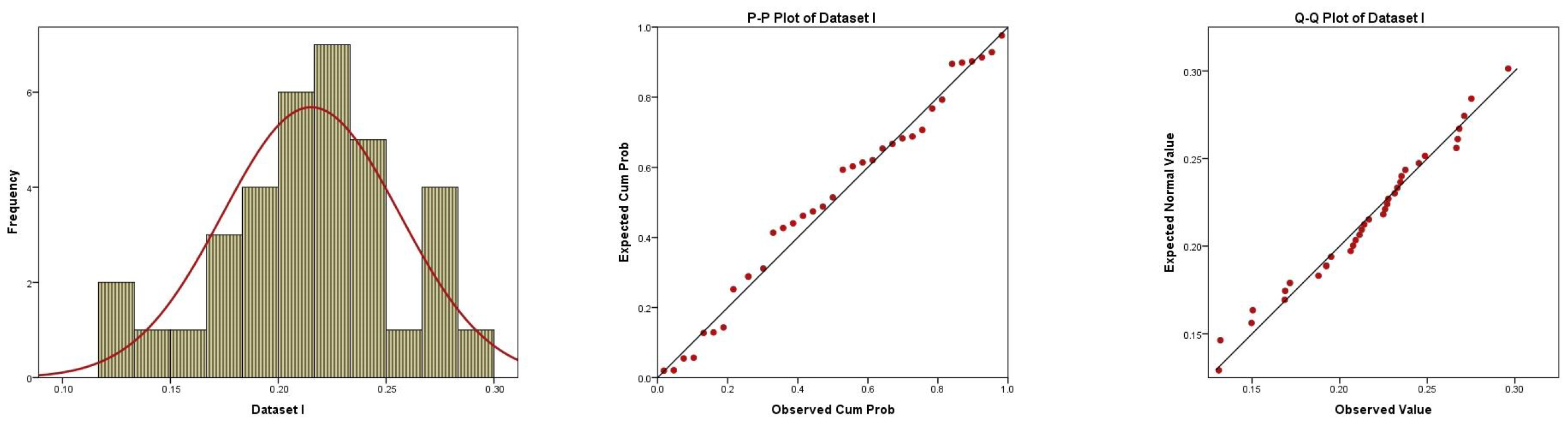
Figure 1 shows the histogram plot with the fitted PDF, P-P plot, and Q-Q plot of the Gumble distribution using dataset I. From this figure, we concluded that the GumD was appropriate for this dataset I. Figure 2 shows three plots of dataset I, where on the left is a boxplot with data explaining that the data had no outlier values, in the middle is an empirical CDF (ECDF) and a theoretical CDF plot with data explaining that the data were increasing, and on the right is a hazard estimated plot line indicating that the hazard was increasing. From Figure 1 and Figure 2, it can be observed that the given dataset I fit the GumD well.

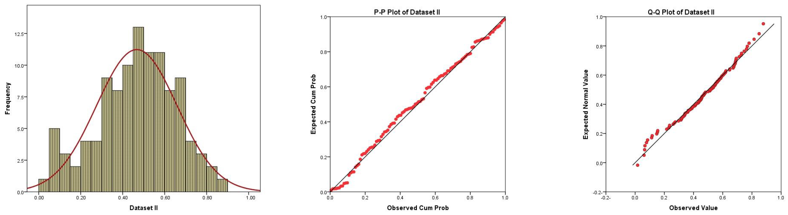
Figure 3 illustrates the histogram graph with the fitted PDF, P-P plot, and Q-Q plot of the GumD based on dataset II. Based on this figure, we concluded that the GumD fit dataset II. Figure 4 displays three graphs of dataset II. The graph on the left shows a boxplot showing the data had no outlier values. The middle graph depicts an empirical CDF and theoretical CDF plot with data indicating that the data were increasing. The right graph depicts a hazard estimated plot line, indicating that the hazard was increasing. From Figure 3 and Figure 4, it was observed that the given dataset II fit the GumD well.

We used the MOM to estimate the unknown parameters of the GumD. During the estimation period, some measurements of error were used, such as $MSE$, mean absolute error ($MAE$), mean bias error ($MBE$), and standard error ($SE$) values, which were calculated using

$$\begin{array}{c}MSE=\frac{1}{n}\sum _{i=1}^n{(x_{obs}-x_{exp})}^2,MAE=\frac{1}{n}\sum _{i=1}^n|x_{obs}-x_{exp}|,\hfill \\ MBE=\frac{1}{n}\sum _{i=1}^n(x_{obs}-x_{exp}),andSE=\sqrt{\frac{1}{n}{\sum }_{i=1}^n{(x_{obs}-x_{exp})}^2},\hfill \end{array}$$

where $x_{obs}$ is the value from a dataset and $x_{exp}$ is the value of x that came from the simulation after estimating the unknown parameters. In

Table 5. The estimators and selected measures for datasets using sampling techniques.

	n	Measures	$\mathit{SRS}$	$\mathit{RSS}$	$\mathit{MRSS}$	$\mathit{OMRSS}$
Dataset I		($\widehat{\alpha },$ $\widehat{\beta }$)	(0.7832, 0.4542)	(0.3848, 0.4559)	(0.3874, 0.3972)	(0.4560, 0.2137)
		$MSE$	1.1499	0.5270	0.4154	0.2356
		$MAE$	0.9304	0.5832	0.4805	0.4367
		$MBE$	1.1499	0.5270	0.4154	0.2356
		$SE$	1.0724	0.7260	0.6445	0.4854
Dataset II		($\widehat{\alpha },$ $\widehat{\beta }$)	(0.5002, 0.3973)	(0.2899, 0.3361)	(0.3091, 0.1852)	(0.6168, 0.2513)
		$MSE$	0.2852	0.1644	0.1301	0.1074
		$MAE$	0.3836	0.3029	0.2896	0.2796
		$MBE$	0.2852	0.1644	0.1301	0.1074
		$SE$	0.5340	0.4055	0.3608	0.3277

, the values of MSE, MAE, MBE, and SE are shown for dataset I with sample size $n=6$ and dataset II with sample size $n=10$ with cycle size $m=1$. Compare the GumD with the SRS, RSS, MRSS, and OMRSS techniques based on the MOM in this table. Based on the results of these measures, we may be able to select the best sample technique for estimating the GumD based on the smaller values of measurements of error. Based on the numerical results of the real datasets, the conclusions can be summarized as follows: First, in general, all measures of error based on the RSS, MRSS, and OMRSS methods were lower than those measures based on the SRS technique. Second, the OMRSS technique was superior to all other sampling techniques. It had the lowest values for the measures of error. Third, it can also be seen that the SRS was inferior to other sampling techniques. It had the highest values measures of error for various estimation techniques. Fourth, the SE had a largest values compared with the other measures of error based on the sampling techniques, while MSE had the lowest values of the measures of error. Finally, the MSE was the same as the MBE for all estimation methods and sampling techniques. It was also the smallest compared with the other measures.

6. Conclusions

In this study, the unknown parameters of Gumbel distribution were estimated using the method of moments based on the SRS, RSS, MRSS, and OMaxRSS techniques. The conclusions can be divided into three parts: First, theoretical results were obtained using the method of moments with sampling techniques. The first and second moments of sampling techniques were obtained and solved numerically to obtain the estimators. Second, based on the comparative study’s simulation results, numerical comparisons between SRS and different RSS techniques revealed that, in general, estimates based on the RSS, MRSS, and OMRSS techniques were more efficient than the SRS estimators. Furthermore, RSS was shown to be less efficient than the MRSS and OMRSS techniques with large MSEs. The OMRSS was more efficient than other SRS-based RSS techniques for different sample sizes. Finally, based on the results of two real datasets used in a comparative study, a numerical comparison between SRS and RSS techniques shows that all measures of error based on the RSS, MRSS, and OMRSS techniques had lower values than those based on the SRS technique. For the sampling techniques, the MSE was the same as the MBE. In comparison with the other measures, the MSE was also the smallest. The RSS had the largest value in the measures compared with the other MRSS and OMRSS techniques. The OMRSS technique was superior to all other sampling techniques; it had the lowest values for the measures of error.

References

- McIntyre, G.A. A method for unbiased selective sampling, using ranked sets. Aust. J. Agric. Res. 1952, 3, 385–390. [Google Scholar] [CrossRef]
- Takahasi, K.; Wakimoto, K. On unbiased estimates of the population mean based on the sample stratified by means of ordering. Ann. Inst. Stat. Math. 1968, 20, 1–31. [Google Scholar] [CrossRef]
- Lavin, M. The ‘Bayesics’ of ranked set sampling. Environ. Ecol. Stat. 1999, 6, 47–57. [Google Scholar] [CrossRef]
- Chen, Z.; Bai, Z.; Sinha, B.K. Ranked Set Sampling: Theory and Applications; Springer: New York, NY, USA, 2004; Volume 176. [Google Scholar]
- Esemen, M.; Gürler, S. Parameter estimation of generalized Rayleigh distribution based on ranked set sample. J. Stat. Comput. Simul. 2018, 88, 615–628. [Google Scholar] [CrossRef]
- Halls, L.K.; Dell, T.R. Trial of ranked-set sampling for forage yields. For. Sci. 1966, 12, 22–26. [Google Scholar]
- Al-Saleh, M.F.; Al-Hadhrami, S.A. Estimation of the mean of the exponential distribution using moving extremes ranked set sampling. Stat. Pap. 2003, 44, 367–382. [Google Scholar] [CrossRef]
- Khamnei, H.J.; Mayan, S.R. Comparison of parameter estimation in the exponentiated Gumbel distribution based on ranked set sampling and simple random sampling. J. Math. Stat. Sci. 2016, 2016, 490–497. [Google Scholar]
- Hassan, N.M.; Rady, E.H.A.; Rashwan, N.I. Estimate the Parameters of the Gamma/Gompertz Distribution based on Different Sampling Schemes of Ordered Sets. J. Stat. Appl. Probab. 2022, 11, 899–914. [Google Scholar]
- Balakrishnan, N.; Li, T. Ordered ranked set samples and applications to inference. J. Stat. Plan. Inference 2008, 138, 3512–3524. [Google Scholar] [CrossRef]
- Stokes, S.L. Inferences on the correlation coefficient in bivariate normal populations from ranked set samples. J. Am. Stat. Assoc. 1980, 75, 989–995. [Google Scholar] [CrossRef]
- Chacko, M. Ordered extreme ranked set sampling and its application in parametric estimation. J. Stat. Theory Appl. 2016, 15, 248–258. [Google Scholar] [CrossRef]
- Eskandarzadeh, M.; Crescenzo, A.D.; Tahmasebi, S. Measures of information for maximum ranked set sampling with unequal samples. Commun. Stat.-Theory Methods 2018, 47, 4692–4709. [Google Scholar] [CrossRef]
- Basikhasteh, M.; Lak, F.; Tahmasebi, S. Ordered maximum ranked set sampling with unequal sample. Statistics 2020, 54, 856–870. [Google Scholar] [CrossRef]
- Biradar, B.S.; Santosha, C.D. Estimation of the mean of the exponential distribution using maximum ranked set sampling with unequal samples. Open J. Stat. 2014, 4, 641. [Google Scholar] [CrossRef]
- Lambert, J.H.; Li, D. Evaluating risk of extreme events for univariate-loss functions. J. Water Resour. Plan. Manag. 1994, 120, 382–399. [Google Scholar] [CrossRef]
- Johnson, N.L.; Kotz, S.; Balakrishnan, N. Continuous Univariate Distributions; John Wiley & Sons: Hoboken, NJ, USA, 1995; Volume 2. [Google Scholar]
- Simiu, E.; Heckert, N.A.; Filliben, J.J.; Johnson, S.K. Extreme wind load estimates based on the Gumbel distribution of dynamic pressures: An assessment. Struct. Saf. 2001, 23, 221–229. [Google Scholar] [CrossRef]
- Kang, D.; Ko, K.; Huh, J. Determination of extreme wind values using the Gumbel distribution. Energy 2015, 86, 51–58. [Google Scholar] [CrossRef]
- Anderson, K.V.; Daniewicz, S.R. Statistical analysis of the influence of defects on fatigue life using a Gumbel distribution. Int. J. Fatigue 2018, 112, 78–83. [Google Scholar] [CrossRef]
- Dutta, S.; Sultana, F.; Kayal, S. Statistical inference for Gumbel type-II distribution under simple step-stress life test using type-II censoring. Iran. J. Sci. 2023, 47, 155–173. [Google Scholar] [CrossRef]
- Hussian, M.A. Bayesian and maximum likelihood estimation for Kumaraswamy distribution based on ranked set sampling. Am. J. Math. Stat. 2014, 4, 30–37. [Google Scholar]
- Sadek, A.; Sultan, K.S.; Balakrishnan, N. Bayesian estimation based on ranked set sampling using asymmetric loss function. Bull. Malays. Math. Sci. Soc. 2015, 38, 707–718. [Google Scholar] [CrossRef]
- Joukar, A.; Ramezani, M.; MirMostafaee, S.M.T.K. Parameter estimation for the exponential-Poisson distribution based on ranked set samples. Commun. Stat. Theory Methods 2021, 50, 560–581. [Google Scholar] [CrossRef]
- Pedroso, V.C.; Taconeli, C.A.; Giolo, S.R. Estimation based on ranked set sampling for the two-parameter Birnbaum–Saunders distribution. J. Stat. Comput. Simul. 2021, 91, 316–333. [Google Scholar] [CrossRef]
- Biradar, B.S. Parametric estimation of location and scale parameters based on ranked set sampling with unequal set sizes. Commun. Stat. Simul. Comput. 2022, 1–16. [Google Scholar] [CrossRef]
- Mahdi, S.; Cenac, M. Estimating Parameters of Gumbel Distribution using the Methods of Moments, probability weighted Moments and maximum likelihood. Rev. Matemática Teoría Apl. 2005, 12, 151–156. [Google Scholar] [CrossRef]
- Choi, B.J. Estimation for scale parameter of type-I extreme value distribution. J. Korean Data Inf. Sci. Soc. 2015, 26, 535–545. [Google Scholar] [CrossRef]
- Fayomi, A.; Hassan, A.S.; Baaqeel, H.; Almetwally, E.M. Bayesian Inference and Data Analysis of the Unit–Power Burr X Distribution. Axioms 2023, 12, 297. [Google Scholar] [CrossRef]
- Zayed, M.A.; Hassan, A.S.; Almetwally, E.M.; Aboalkhair, A.M.; Al-Nefaie, A.H.; Almongy, H.M. A Compound Class of Unit Burr XII Model: Theory, Estimation, Fuzzy, and Application. Sci. Program. 2023, 2023, 4509889. [Google Scholar] [CrossRef]
Figure 1.
Histogram, P-P plot, and Q-Q plot for the fit of GumD based on dataset I.
Figure 2.
Boxplot, ECDF, and hazard plot for the fit of GumD based on dataset I.
Figure 3.
Histogram, P-P plot, and Q-Q plot for the fit of GumD based on dataset II.
Figure 4.
Boxplot, ECDF, and hazard plot for the fit of GumD based on dataset II.