Matching the LBO Eigenspace of Non-Rigid Shapes via High Order Statistics

Abstract

A fundamental tool in shape analysis is the virtual embedding of the Riemannian manifold describing the geometry of a shape into Euclidean space. Several methods have been proposed to embed isometric shapes into flat domains, while preserving the distances measured on the manifold. Recently, attention has been given to embedding shapes into the eigenspace of the Laplace–Beltrami operator. The Laplace–Beltrami eigenspace preserves the diffusion distance and is invariant under isometric transformations. However, Laplace–Beltrami eigenfunctions computed independently for different shapes are often incompatible with each other. Applications involving multiple shapes, such as pointwise correspondence, would greatly benefit if their respective eigenfunctions were somehow matched. Here, we introduce a statistical approach for matching eigenfunctions. We consider the values of the eigenfunctions over the manifold as the sampling of random variables and try to match their multivariate distributions. Comparing distributions is done indirectly, using high order statistics. We show that the permutation and sign ambiguities of low order eigenfunctions can be inferred by minimizing the difference of their third order moments. The sign ambiguities of antisymmetric eigenfunctions can be resolved by exploiting isometric invariant relations between the gradients of the eigenfunctions and the surface normal. We present experiments demonstrating the success of the proposed method applied to feature point correspondence.

1. Introduction

The embedding of nonrigid shapes into a Euclidean space is well established and widely used by shape analysis applications. Usually, the mapping from the manifold to the Euclidean space preserves distances, that is the distance measured between two points on the manifold is approximated by the respective distance calculated in the Euclidean space. The embedding of multiple isometric shapes into the same common Euclidean space seems to be ideal for applications like pointwise correspondence and shape editing. A useful property of this common embedding would be if any corresponding points of different isometric shapes were mapped to nearby target points in the Euclidean space. If this property is fulfilled, then the simultaneous processing of shapes in the target domain can be done in a straightforward manner.

Elad et al. [1] used classical multi-dimensional scaling (MDS) embedding into the geodesic kernel eigenspace. The MDS dissimilarity measure was based on the geodesic distances computed by the fast marching procedure [2]. Bérard et al. [3] used the heat operator spectral decomposition to define a metric between two manifolds M and $M^{\prime }$. They embedded the two manifolds into their respective eigenspaces, and measured the Hausdorff distance [4] between the two shapes in the spectral domain. The Hausdorff distance $d_H(M,M^{\prime })$, being the greatest of all the distances from a point in one set to the closest point in the other set, can easily be calculated in this common Euclidean space. They showed that $d_H(M,M^{\prime })=0$ if and only if the Riemannian manifolds M and $M^{\prime }$ are isometric. Lafon et al. [5] defined the diffusion maps and showed that the embedding into the heat kernel eigenspace is isometry invariant and preserves the diffusion metric. Rustamov [6] introduced the global point signature (GPS) embedding for deformation-invariant shape representation.

Although the diffusion maps computed independently on isometric shapes have a nearly compatible eigenbasis, several inconsistencies arise:

• Eigenfunctions are defined up to a sign.
• The order of the eigenfunctions, especially those representing higher frequencies, is not repeatable across shapes.
• The eigenvalues of the Laplace–Beltrami operator may have a multiplicity greater than one, with several eigenfunctions corresponding to each such eigenvalue.
• It is generally impossible to expect that an eigenfunction with a large eigenvalue of one shape will correspond to any eigenfunction of another shape.
• Intrinsic symmetries introduce self-ambiguity, adding complexity to the sign estimation challenge.

These drawbacks limit the use of diffusion maps in simultaneous shape analysis and processing; they do not allow using high frequencies and usually require some intervention to order the eigenfunctions or solve sign ambiguities.

In this paper, we present a novel method for matching eigenfunctions that were independently calculated for two nearly isometric shapes. We rely on the fact that for low order eigenfunctions, inconsistencies are usually governed by a small number of discrete parameters characterized by the sign sequence and permutation vector. We estimate these parameters by matching statistical properties over the spectral domain. The matching of the corresponding eigenfunctions enables the use of diffusion maps for consistent embedding of multiple isometric shapes into a common Euclidean space.

1.1. Related Work

The problems of eigenfunctions permutation and sign ambiguity were previously addressed in the context of simultaneous shape processing. Several authors, among them Shapiro and Brady [7] and Jain et al. [8], proposed using either exhaustive search or a greedy approach for the eigenvalue ordering and sign detection. Umeyama [9] proposed using a combination of the absolute values of the eigenfunctions and an exhaustive search. Mateus et al. [10] expressed the connection between the eigenfunctions of two shapes by an orthogonal matrix. They formulated the matching as a global optimization problem, optimizing over the space of orthogonal matrices, and solved it using the expectation minimization approach. Later, Mateus et al. [11] and Knossow et al. [12] suggested using histograms of eigenfunctions values to detect their ordering and signs. Dubrovina et al. [13] suggested using a coarse matching based on absolute values of eigenfunctions together with geodesic distances measured on the two shapes.

Most of these methods do not reliably resolve eigenfunction permutation [7,8,10,12]. Some of the above algorithms are limited by high complexity and do not allow the matching of more than a few eigenfunctions [9,13]. None of these methods reliably estimate the sign sequence of antisymmetric eigenfunctions.

At the other end, Kovnatsky et al. [14] proposed avoiding the matching problem by constructing a common approximate eigenbases for multiple shapes using approximate joint diagonalization algorithms. Yet, it relies on prior knowledge of a set of corresponding feature points.

Finally, the algorithm proposed by Pokrass et al. [15] mostly resembles our approach. They used sparse modeling to match the Laplace–Beltrami operator (LBO) eigenfunctions that span the wave kernel signature (WKS). Yet, that approach does not reliably infer the signs of the antisymmetric eigenfunctions.

1.2. Background

1.2.1. Laplace–Beltrami Eigendecomposition

Let us be given a shape modeled as a compact two-dimensional manifold M. The divergence of the gradient of a function f over the manifold:

$${\Delta }_{G}f=\mathrm{div}\mathrm{grad}f$$

(1)

is called the Laplace–Beltrami operator (LBO) of f and can be considered as a generalization of the standard notion of the Laplace operator to manifolds [16,17]. The Laplace–Beltrami operator is completely derived from the metric tensor G.

$${\Delta }_{G}f=divgradf=\underset{divergence}{\underbrace{\frac{1}{\sqrt{\left|G\right|}}\sum _i{\partial }_i\sqrt{\left|G\right|}}}\underset{gradient}{\underbrace{\sum _j{g}^{ij}{\partial }_j}}f$$

(2)

where $g^{ij}={\left(G^{-1}\right)}_{ij}$ are the components of the inverse metric tensor.

Since the operator $-{\Delta }_G$ is a positive self-adjoint operator, it admits an eigendecomposition with non-negative eigenvalues ${\lambda }_i$ and corresponding orthonormal eigenfunctions ${\varphi }_i$,

$$-{\Delta }_G{\varphi }_i={\lambda }_i{\varphi }_i$$

(3)

where orthonormality is understood in the sense of the local inner product induced by the Riemannian metric on the manifold. Furthermore, due to the assumption that our manifold is compact, the spectrum is discrete. We can order the eigenvalues as follows $0={\lambda }_1<{\lambda }_2<\cdots <{\lambda }_i<\cdots$. The set of corresponding eigenfunctions given by $\{{\varphi }_1,{\varphi }_2,\cdots ,{\varphi }_i,\cdots \}$ forms an orthonormal basis of functions defined on M.

1.2.2. Diffusion Maps

The heat equation describes the distribution of heat in time. On a manifold M, the heat equation is governed by the Laplace–Beltrami operator ${\Delta }_G$:

$$\frac{\partial u}{\partial t}={\Delta }_{G}u$$

(4)

The heat kernel $K_t(x,y)$ is the diffusion kernel of the heat operator $e^{t{\Delta }_G}(t>0)$. It is a fundamental solution of the heat equation with the point heat source at x (the heat value at point y after time t). The heat kernel can be represented in the Laplace–Beltrami eigenbasis as:

$$K_t(x,y)=\sum _i{\left({\tilde{\lambda }}_i\right)}^t{\varphi }_i\left(x\right){\varphi }_i\left(y\right)=\sum _i{e}^{-{\lambda }_{i}t}{\varphi }_i\left(x\right){\varphi }_i\left(y\right)$$

(5)

where ${\tilde{\lambda }}_i$ are the eigenvalues of the heat operator, ${\lambda }_i$ are the eigenvalues of the LBO and ${\tilde{\lambda }}_i=e^{-{\lambda }_i}$.

Using the heat kernel, we can define the diffusion distance [5]:

$$\begin{array}{cc}\hfill d_{M,t}^2(x,y)& =\left|\right|K_t(x,·)-K_t(y,·){\left|\right|}_{L^2}^2\hfill \\ & ={\int }_M{(K_t(x,z)-K_t(y,z))}^{2}da\left(z\right)\hfill \end{array}$$

(6)

where $da$ is the area element of M.

The diffusion distance $d_{M,t}(x,y)$ can be computed by embedding the manifold into the infinite Euclidean space spanned by the LBO eigenbasis:

$$d_{M,t}(x,y)={\left(\sum _i{e}^{-2{\lambda }_{i}t}{({\varphi }_i\left(x\right)-{\varphi }_i\left(y\right))}^2\right)}^{\frac{1}{2}}$$

(7)

The diffusion map $\left\{{\Phi }_t\right\}$ embeds the data into the finite N-dimension Euclidean space:

$${\Phi }_t\left(x\right)=\left[\begin{array}{c}{e}^{-{\lambda }_{1}t}{\varphi }_1\left(x\right)\\ e^{-{\lambda }_{2}t}{\varphi }_2\left(x\right)\\ ...\\ e^{-{\lambda }_{N}t}{\varphi }_N\left(x\right)\end{array}\right]$$

(8)

so that in this space, the Euclidean distance is equal to the diffusion distance up to a relative truncation error:

$$d_{M,t}(x,y)\approx \left|\right|{\Phi }_t\left(x\right)-{\Phi }_t\left(y\right)\left|\right|$$

(9)

1.2.3. Multivariate Distribution Comparison

The distribution of N continuous random variables ${\varphi }_1,{\varphi }_2,...,{\varphi }_N$ is directly represented by the probability density function $f_{{\varphi }_1,{\varphi }_2,...,{\varphi }_N}({\varphi }_1,{\varphi }_2,...,{\varphi }_N)$. The direct estimation of the multivariate probability density function from data samples is hard to accomplish. Therefore, instead of using a direct comparison of distribution functions [18,19], an indirect representation is often being utilized. The probability distribution can be indirectly specified (under mild conditions) in a number of different ways, the simplest of which is by its raw moments:

$${\mu }_{i_1,i_2,...,i_N}\equiv E[{\varphi }_1^{i_1}{\varphi }_2^{i_2}...{\varphi }_N^{i_N}],\{i_1,i_2,...,i_N\}\in {\mathbb{Z}}_{\ge 0}$$

(10)

In order to compare the multivariate distributions of two sets of N random variables ${\varphi }_1^X,{\varphi }_2^X,...,{\varphi }_N^X$ and ${\varphi }_1^Y,{\varphi }_2^Y,...,{\varphi }_N^Y$, we can use this indirect representation and compare the raw moments of the random variables. In practice, only a small set of the moments $\mathcal{I}$ can be used for measuring the difference between the distributions:

$$\begin{array}{cc}\hfill C_{X,Y}& =\sum _{\{i_1,i_2,...,i_N\}\in \mathcal{I}}{\rho }_{i_1,i_2,...,i_N}{({\mu }_{i_1,i_2,...,i_N}^X-{\mu }_{i_1,i_2,...,i_N}^Y)}^2\hfill \end{array}$$

(11)

where ${\rho }_{i_1,i_2,...,i_N}$ are the weights associated with each raw moment.

2. Eigenfunction Matching

2.1. Problem Formulation

Let us denote by X and Y the two shapes that we would like to match. We represent the correspondence between X and Y by a bijective mapping $\phi :X\mapsto Y$, such that for each point $x\in X$, its corresponding point is $\phi \left(x\right)\in Y$. The diffusion map embeds each point $x\in X$ into the N dimension Euclidean space ${\mathbb{R}}^N$ according to ${\Phi }_t^{X,N}\left(x\right)$. Correspondingly, each point $y\in Y$ is embedded by the mapping ${\Phi }_t^{Y,N}\left(y\right)$ into ${\mathbb{R}}^N$. We denote the diffusion map at $t=0$ by ${\Phi }^X\left(x\right)={\Phi }_{t=0}^{X,N}\left(x\right)$ and ${\Phi }^Y\left(y\right)={\Phi }_{t=0}^{Y,N}\left(y\right)$, respectively.

We wish to find embeddings of shape X and shape Y to the finite dimensional Euclidean space, such that the corresponding points $x\in X$ and $\phi \left(x\right)\in Y$ will be mapped to nearby points in the embedded space. Because of the inconsistencies described in the Introduction, the diffusion maps of shapes X and Y do not necessarily fulfill this property. Our task is to modify the diffusion map ${\Phi }^Y\left(y\right)$ by a small number of parameters θ, such that the new embedding ${\tilde{\Phi }}_{\theta }^Y\left(y\right)$ will match ${\Phi }^X$, i.e., ${\Phi }^X\left(x\right)\approx {\tilde{\Phi }}_{\theta }^Y\left(\phi \left(x\right)\right)$.

For the N low eigenvalues, the matching is characterized by the following parameters:

• The respective signs of the eigenfunctions $\mathbf{s}:s_i\in \{+1,-1\}$.
• The permutation vector π of the eigenfunctions: $\pi :\{1,2,...,N\}\mapsto \{1,2,...,N\}$.

We would like to find the parameters $\widehat{\theta }=\{\widehat{\mathbf{s}};\widehat{\mathit{\pi }}\}$, which create the matched embedding ${\tilde{\Phi }}_{\widehat{\theta }}^Y\left(y\right)$ with elements ${\tilde{\varphi }}_i^Y={\widehat{s}}_i{\varphi }_{\widehat{\pi }\left(i\right)}^Y,i\in 1,2,...N$.

2.2. Matching Cost Function

The entire algorithm can be expressed as the minimization of the following cost function:

$$\{\widehat{\mathbf{s}};\widehat{\mathit{\pi }}\}={\mathrm{argmin}}_{\mathbf{s};\mathit{\pi }}(C(\mathbf{s},\mathit{\pi })+C^S(\mathbf{s},\mathit{\pi })+\alpha (C_{\nabla }^P(\mathbf{s},\mathit{\pi })+C_{\nabla }^{P,S}(\mathbf{s},\mathit{\pi })))$$

(12)

2.2.1. Overview

The objective function is comprised of four terms $C,C^S,C_{\nabla }^P,C_{\nabla }^{P,S}$. The first and second terms (C, $C^S$) compare the mixed moments of compatible functions. Minimizing the terms C, $C^S$ is usually sufficient to correctly reorder the eigenfunctions and find the right sign sequence. Alas, in the presence of intrinsic symmetry, these mixed moments are ambiguous and cannot be compared effectively. The third and fourth terms ($C_{\nabla }^P$, $C_{\nabla }^{P,S}$) work out this difficulty by using a pair of gradients of compatible functions. The gradients are inserted into the functional, by incorporating their cross-product in the direction of the outward pointing normal to the surface.

To enhance the discriminative properties of the algorithm and its robustness, we apply two additional techniques.

⋄

Pointwise signatures as side information: We mix in stable compatible signatures, like the heat kernel signature (HKS), employed in $C^S$, $C_{\nabla }^P$, $C_{\nabla }^{P,S}$.

⋄

Raw moments over segments: We blindly (i.e. , without correspondence) segment the shapes into parts in a compatible way and integrate over these segments separately; employed in $C_{\nabla }^P$, $C_{\nabla }^{P,S}$.

2.2.2. Cost Function Terms

The terms of the cost function can be expressed by:

• $C(\mathbf{s},\mathit{\pi })={\displaystyle \sum _{i,j,k}}{({\mu }_{i,j,k}^X-s_i{s}_j{s}_k{\mu }_{\pi \left(i\right),\pi \left(j\right),\pi \left(k\right)}^Y)}^2$

  • ${\mu }_{i,j,k}=E\left[{\varphi }_i{\varphi }_j{\varphi }_k\right],i,j,k\in \{1,2,...,N\}$
• $C_{\nabla }^P(\mathbf{s},\mathit{\pi })={\displaystyle \sum _{i,j,k,p}}{({\xi }_{i,j,k,p}^X-s_i{s}_j{s}_k{\xi }_{\pi \left(i\right),\pi \left(j\right),\pi \left(k\right),p}^Y)}^2$

  • ${\xi }_{i,j,k,p}=E[{\nu }_{i,j}{\varphi }_k{w}_p\left(\right|{\varphi }_k\left|\right)],$
  • $i,j,k\in \{1,2,...,N\},p\in \{1..P\}$
  • ${\nu }_{i,j}=({\nabla }_G{\varphi }_i\times {\nabla }_G{\varphi }_j)·\mathbf{n}$
• $C^S(\mathbf{s},\mathit{\pi })=N{\displaystyle \sum _{i,q}}{({\mu }_{i,q}^{X,S}-s_i{\mu }_{\pi \left(i\right),q}^{Y,S})}^2$

  • ${\mu }_{i,q}^S=E\left[{\varphi }_i{\psi }_q\right],i\in \{1,2,...,N\},q\in \{1,2,...Q\}$
• $C_{\nabla }^{P,S}(\mathbf{s},\mathit{\pi })={\displaystyle \sum _{i,q,k,p}}{({\xi }_{i,q,k,p}^{X,S}-s_i{s}_k{\xi }_{\pi \left(i\right),q,\pi \left(k\right),p}^{Y,S})}^2$

  • ${\xi }_{i,q,k,p}^S=E[{\nu }_{i,q}^S{\varphi }_k{w}_p\left(\right|{\varphi }_k\left|\right)],$
  • $i,k\in \{1..N\},p\in \{1..P\},q\in \{1..Q\}$
  • ${\nu }_{i,q}^S=({\nabla }_G{\varphi }_i\times {\nabla }_G{\psi }_q)·\mathbf{n}$

where:

• ${\varphi }_i$ are the eigenfunctions of the Laplace–Beltrami operator $-{\Delta }_G{\varphi }_i={\lambda }_i{\varphi }_i$.
• $w_p:{\mathbb{R}}_{\ge 0}\mapsto [0,1]$ are nonlinear weighting functions.
• ${\psi }_q:M\mapsto \mathbb{R}$ are the components of an external point signature.
• ${\nabla }_G$ is the gradient induced by the metric tensor G.
• $E\left[z\right]={\int }_{M}zd{a}_M$, where $d{a}_M$ is the area element of the manifold M.
• $\mathbf{n}$ is the normal to the surface.
• × is the cross-product in ${\mathbb{R}}^3$, and · is the inner product in ${\mathbb{R}}^3$.
• The weighting parameter α determines the relative weight of the gradient cost functions.

In Appendix A1, we give full details of the discretization that we have used to implement the matching algorithm.

The application specific parameters include:

• N: the number of eigenfunctions to be matched.
• ${\left\{w_p\right\}}_{p=1}^P$: the P nonlinear weighting functions.
• ${\left\{{\psi }_q\right\}}_{q=1}^Q$: the external point signature of size Q.
• α: the relative weight of the gradient cost functions.

In Appendix A2, we give the details of the application specific parameters that were used in our experiments.

Next, we review the different terms of the cost function.

2.2.3. Resolving Sign Ambiguities and Permutations

For now, let us limit our discussion to resolving the sign ambiguity $\mathbf{s}$. If we had known the correspondence between the two shapes, the sign of the $i-th$ eigenfunction $s_i$ could be inferred by pointwise comparison:

$${\widehat{s}}_i={\mathrm{argmin}}_{s_i}E[({\varphi }_i^X\left(x\right)-s_i{\varphi }_i^Y{\left(\phi \left(x\right)\right)}^2]$$

(13)

and the expectation is taken over the manifold:

$$E\left(f\left(x\right)\right)={\int }_{X}f\left(x\right)d{a}_X$$

(14)

where $d{a}_X$ is the area element of the shape X. Unfortunately, the correspondence is unknown. Hence, pointwise comparison cannot be used in a straightforward manner.

We now make the analogy between the values of the eigenfunctions over the manifold and N random variables. We consider the vector of values of the diffusion map ${\Phi }^X\left(x\right)$ at point x as a sample out of a multivariate distribution $f_{\Phi }({\varphi }_1\left(x\right),{\varphi }_2\left(x\right),...,{\varphi }_N\left(x\right))$. We wish to match the multivariate distributions $f_{{\Phi }^X}$ and $f_{{\Phi }_{\theta }^Y}$. As explained in Section 1.2.3., an indirect representation of the distribution is suitable for comparing multivariate distributions. Specifically, we shall use the raw moments.

By way of construction, the non-trivial eigenfunctions have zero mean and are orthonormal. Hence, the first and second moments carry no information. Accordingly, we must use higher order moments to match the distributions. We propose to use the third order moments over the manifold M

$$\begin{array}{cc}\hfill {\mu }_{i,j,k}& =E\left[{\varphi }_i{\varphi }_j{\varphi }_k\right]={\int }_M{\varphi }_i{\varphi }_j{\varphi }_{k}d{a}_M\hfill \\ & i,j,k\in \{1,2,...,N\}\hfill \end{array}$$

(15)

2.2.4. Resolving Antisymmetric Eigenfunctions

For shapes with intrinsic symmetries (see [20]), some of the eigenfunctions have antisymmetric distributions. The distribution of the antisymmetric eigenfunctions is agnostic to sign change. Hence, the signs of the antisymmetric eigenfunctions cannot be resolved by the simple scheme described in Section 2.2.3.

The gradient of the eigenfunctions $\nabla {\varphi }_k$ could be exploited to resolve the sign ambiguity:

• The gradient $\nabla f$ of an antisymmetric eigenfunction f is not antisymmetric.
• The gradient is a linear operator. Consequently $\nabla (-f)=-\nabla f,\forall f$.

Therefore, we can farther expand the set of variables that are used in the calculation of the raw moments, by incorporating the gradient. The gradient vector is contained in the tangent plane. Thus, the cross-product of the gradients of two eigenfunctions points either outward or inward from an orientable surface. Changing the sign of one eigenfunction will flip the direction of the cross-product. We can use this property to define new functions ${\nu }_{i,j}$ over the manifold:

$${\nu }_{i,j}=(\nabla {\varphi }_i\times \nabla {\varphi }_j)·\mathbf{n}$$

(16)

where $\mathbf{n}$ is the outward pointing normal to the tangent plane. We shall use the joint moments of the eigenfunctions and their gradients:

$${\xi }_{i,j,k}=E\left[{\nu }_{i,j}{\varphi }_k\right],i,j,k\in \{1,2,...,N\}$$

(17)

We note that Equation (16) can be further simplified by:

$${\nu }_{i,j}=(\nabla {\varphi }_i\times \nabla {\varphi }_j)·\mathbf{n}=\nabla {\varphi }_i·(\nabla {\varphi }_j\times \mathbf{n})$$

(18)

$(\nabla {\varphi }_j\times \mathbf{n})$ can be computed only once for each ${\varphi }_j$.

2.2.5. Raw Moments over Segments

Taking the expectation over the whole shape may be too crude, especially for detecting antisymmetric sign ambiguities. We can refine the minimization criterion by taking the expectation over different segments of the shapes. Remember that the correspondence between the shapes is yet unknown; therefore, directly dividing the shape into corresponding segments is impossible. Indirectly dividing the shape into different segments is possible by using the eigenfunctions themselves. The eigenfunctions ${\varphi }_k$, $k\in \{1...N\}$ have respective low eigenvalues, which means that they have a slow rate of change. Therefore, it is possible to define indicator functions $w_p\left(\right|{\varphi }_k\left(x\right)\left|\right):X\to \{0,1\}$, $p\in \{1..P\}$ in a way that will output one or zero values at different segments of the shape. For example, we can define $h\left(\right|{\varphi }_k\left(x\right)\left|\right)=1\text{if}|{\varphi }_k\left(x\right)|>\text{TH}\text{and}\text{zero}\text{otherwise}$, where TH is a scalar threshold. The output of these functions automatically divides the two shapes into a similar manner, without the use of pointwise correspondence. Moreover, because the function $w_p\left(\right|{\varphi }_k\left|\right)$ is symmetric, its output does not depend on the sign of the eigenfunction ${\varphi }_k$. We conclude that we can use $w_p\left(\right|{\varphi }_k\left|\right)$ to make a weighted average of the raw moments according to different segments:

$$\begin{array}{cc}\hfill {\xi }_{i,j,k,p}& =E[{\nu }_{i,j}{\varphi }_k{w}_p\left(\right|{\varphi }_k\left|\right)]\hfill \\ & i,j,k\in \{1,2,...,N\},p\in \{1..P\}\hfill \end{array}$$

(19)

2.2.6. Pointwise Signatures As Side Information

We can easily use other signatures $({\psi }_1,{\psi }_2,...,{\psi }_Q)$ as side information to refine the minimization criterion. Specifically, we can use signatures that carry no inconsistencies among different shapes. In our experiments, we used the heat kernel signature (HKS) as an additional signature [21]. We can use the joint moments of the diffusion maps and the additional signatures ${\psi }_q$:

$${\mu }_{i,q}^S=E\left[{\varphi }_i{\psi }_q\right],i\in \{1,2,...,N\},q\in \{1,2,...Q\}$$

(20)

and compute the cross of the eigenfunctions gradient $\nabla {\varphi }_i$ and the signature functions gradients $\nabla {\psi }_q$:

$${\nu }_{i,q}^S=(\nabla {\varphi }_i\times \nabla {\psi }_q)·\mathbf{n}$$

(21)

$$\begin{array}{cc}\hfill {\xi }_{i,q,k,p}^S& =E[{\nu }_{i,q}^S{\varphi }_k{w}_p\left(\right|{\varphi }_k\left|\right)]\hfill \\ & i,k\in \{1,2,...,N\},p\in \{1..P\},q\in \{1..Q\}\hfill \end{array}$$

(22)

2.3. Solving the Minimization Problem

The minimization of Equation (12) is a non-convex optimization problem. Yet, it only involves a small number of discrete parameters. Therefore, an exhaustive search is possible. In practice, we implemented the search in four steps:

• Step 1: An initialization of ${\mathbf{s}}^{\mathbf{0}}$ is determined by $s_i=sign\left({\mu }_{i,i,i}^X{\mu }_{i,i,i}^Y\right)$ and ${\mathit{\pi }}^{\mathbf{0}}=[0,1,...N]$.
• Step 2: The permutation vector $\widehat{\pi }$ is found by minimizing $C(\mathbf{s},\mathit{\pi })+C^S(\mathbf{s},\mathit{\pi })$. We make an educated guess for the possible permutations, limiting the search for two permutation profiles:

  ⋄

  two consecutive eigenfunction switching (with possible sign change), i.e., $[{\pi }_i,{\pi }_j,{\pi }_k,{\pi }_l]=[j,i,l,k],j=i+1,l=k+1$

  ⋄

  triplet permutation (with possible sign change), i.e., $[{\pi }_i,{\pi }_j,{\pi }_k]=[j,k,i]$ or $[k,i,j],j=k+1,i=j+1$;

• Step 3: The sign sequence is resolved again by minimizing $C(\mathbf{s},\mathit{\pi })+C^S(\mathbf{s},\mathit{\pi })$. In this step, all possible quadruple sign changes are checked, setting the permutation vector found in Step 2. If the cost function was decreased in Step 2 or Step 3, then return to Step 2. While finding the optimal sign sequence and permutation vector, we keep a list of all possible good sign sequences for the next step.
• Step 4: The optimal sign sequence $\widehat{\mathbf{s}}$ is found by comparing the entire cost function $C(\mathbf{s},\mathit{\pi })+C^S(\mathbf{s},\mathit{\pi })+\alpha (C_{\nabla }^P(\mathbf{s},\mathit{\pi })+C_{\nabla }^{P,S}(\mathbf{s},\mathit{\pi }))$ for each sign sequence in the list created in Step 3.

3. Results

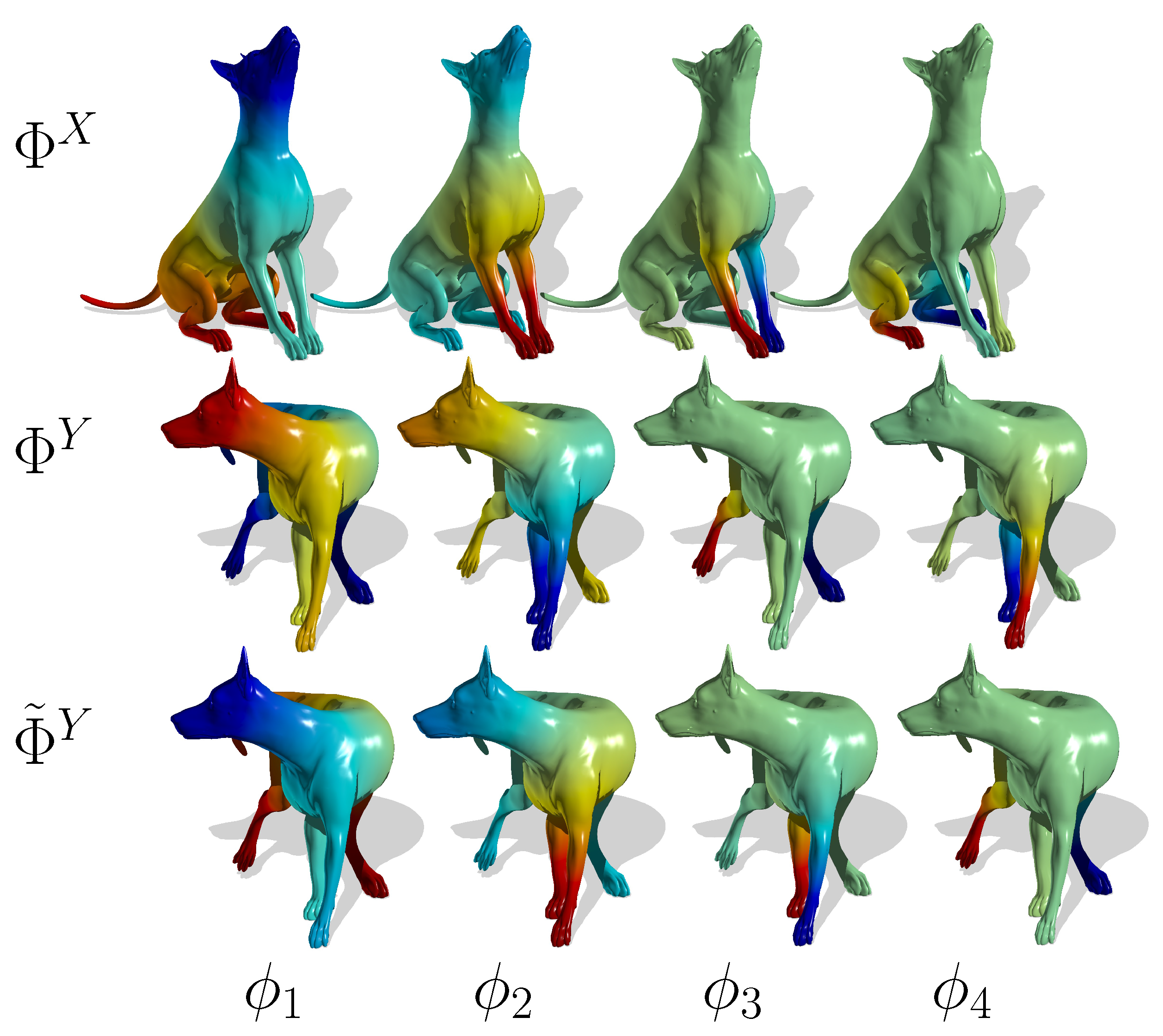
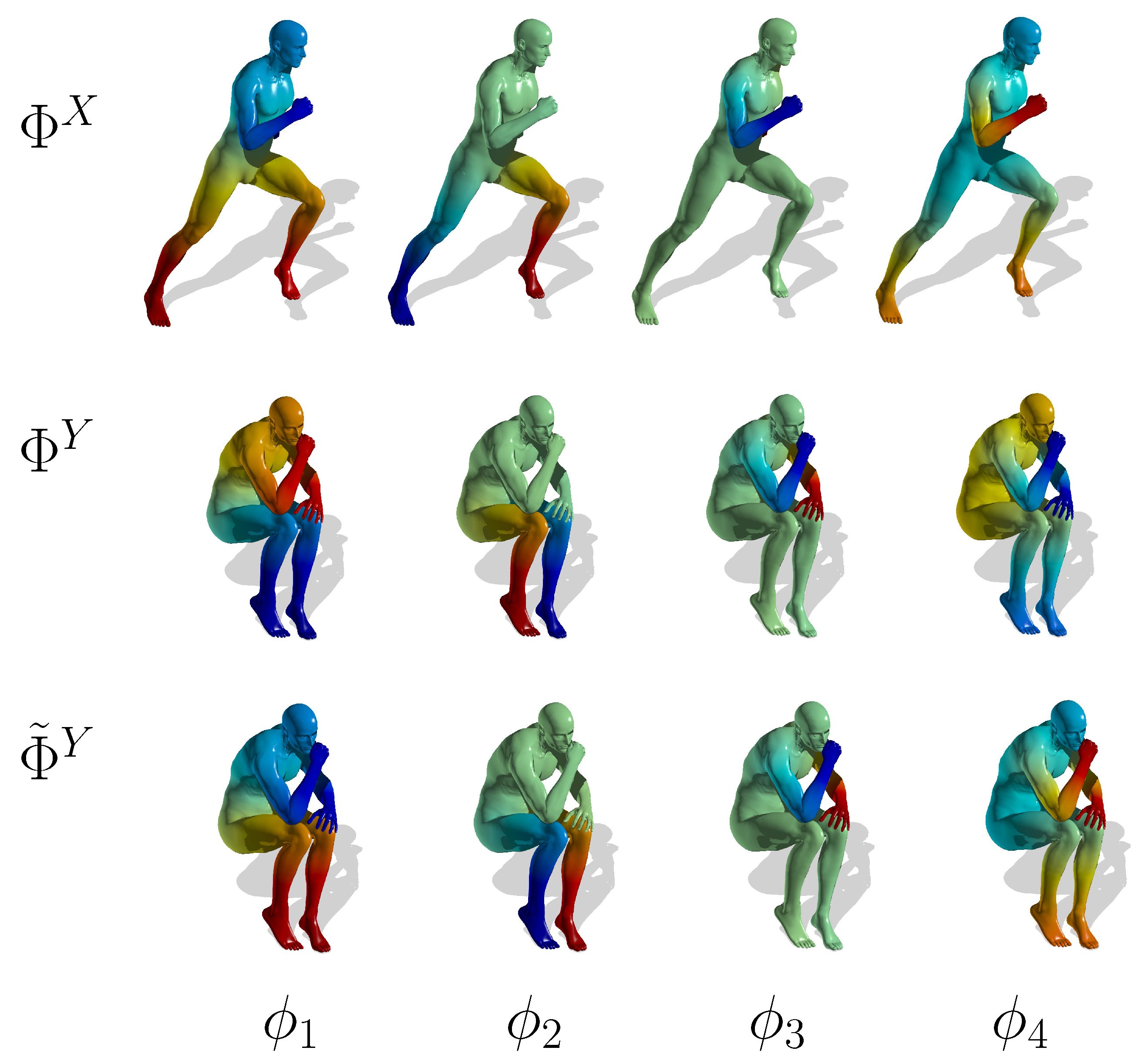
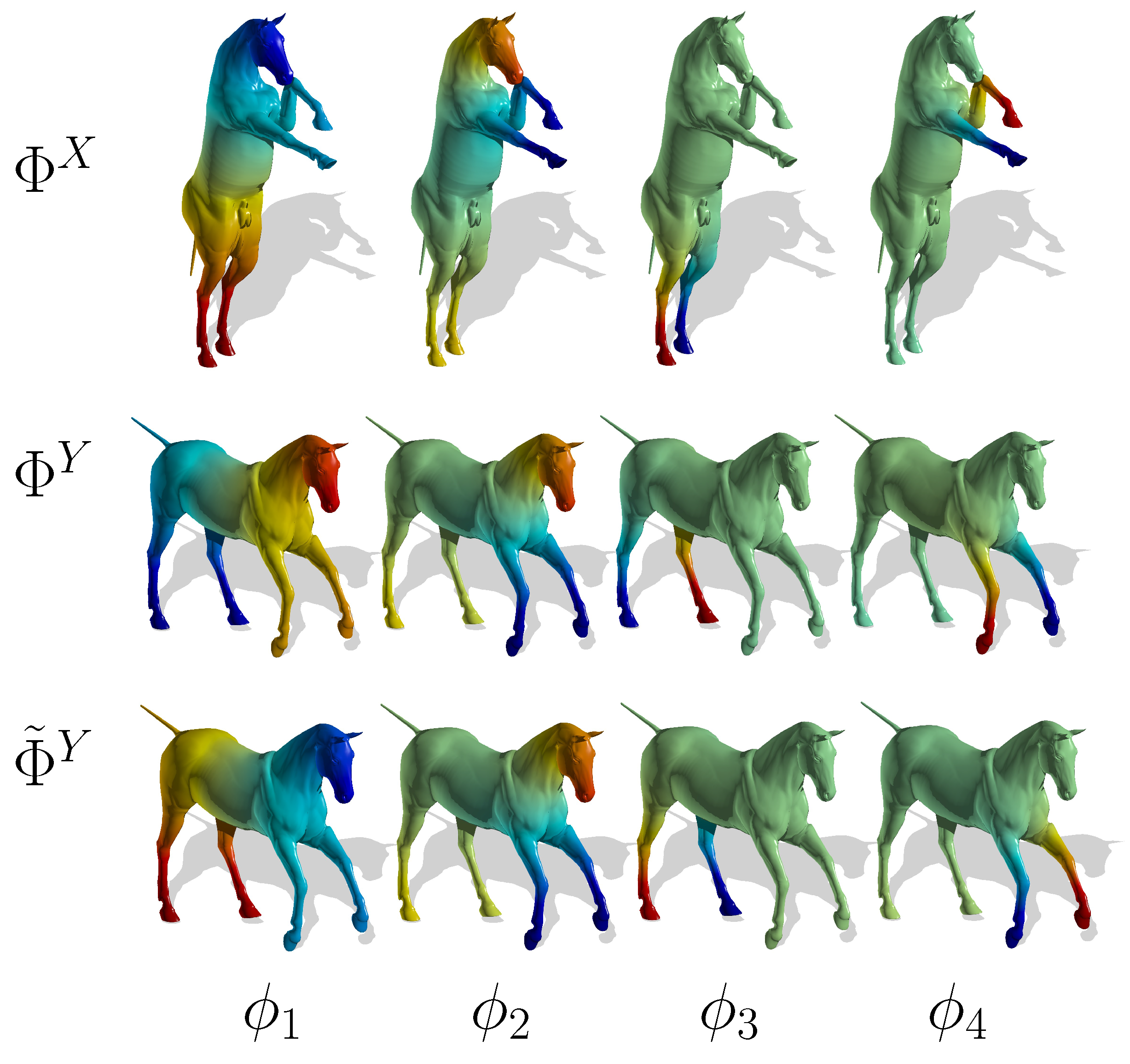
We tested the proposed method on pairs of shapes represented by triangulated meshes from the TOSCA database [22]. Figure 1, Figure 3 and Figure 5 show how the proposed method succeeds in matching the eigenfunctions of several isometric shapes. In each figure, at the top, are the first four eigenfunctions of the first pose of the object. In the middle are the eigenfunctions of the second pose of the object. At the bottom are the first four eigenfunctions of the second pose with the correct sign sequence and permutations.

For example, we can see in Figure 1 that the eigenfunction matching algorithm swapped ${\varphi }_3^Y$ and ${\varphi }_4^Y$. It also correctly flipped the signs of ${\varphi }_1^Y$, ${\varphi }_2^Y$ and ${\varphi }_4^Y$. We also notice that the matching algorithm was able to detect the correct signs of the antisymmetric eigenfunctions. For example, in Figure 3, the sign of the antisymmetric eigenfunction ${\varphi }_2^Y$ was correctly flipped, while keeping the sign of ${\varphi }_3^Y$.

We used the matched eigenfunctions for detecting feature point correspondence between the two shapes. A selected number of feature points from the first shape were matched to the second one using a combination of two signatures:

• The matched low order eigenfunctions that represent the global structure of the shapes.
• The heat kernel signature (HKS) derivative (Equation (A11)) that, being a bandpass filter, expresses more local features.

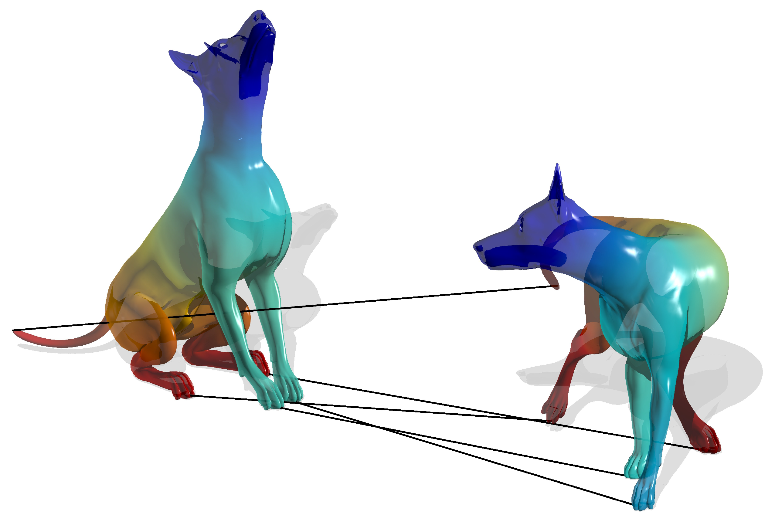
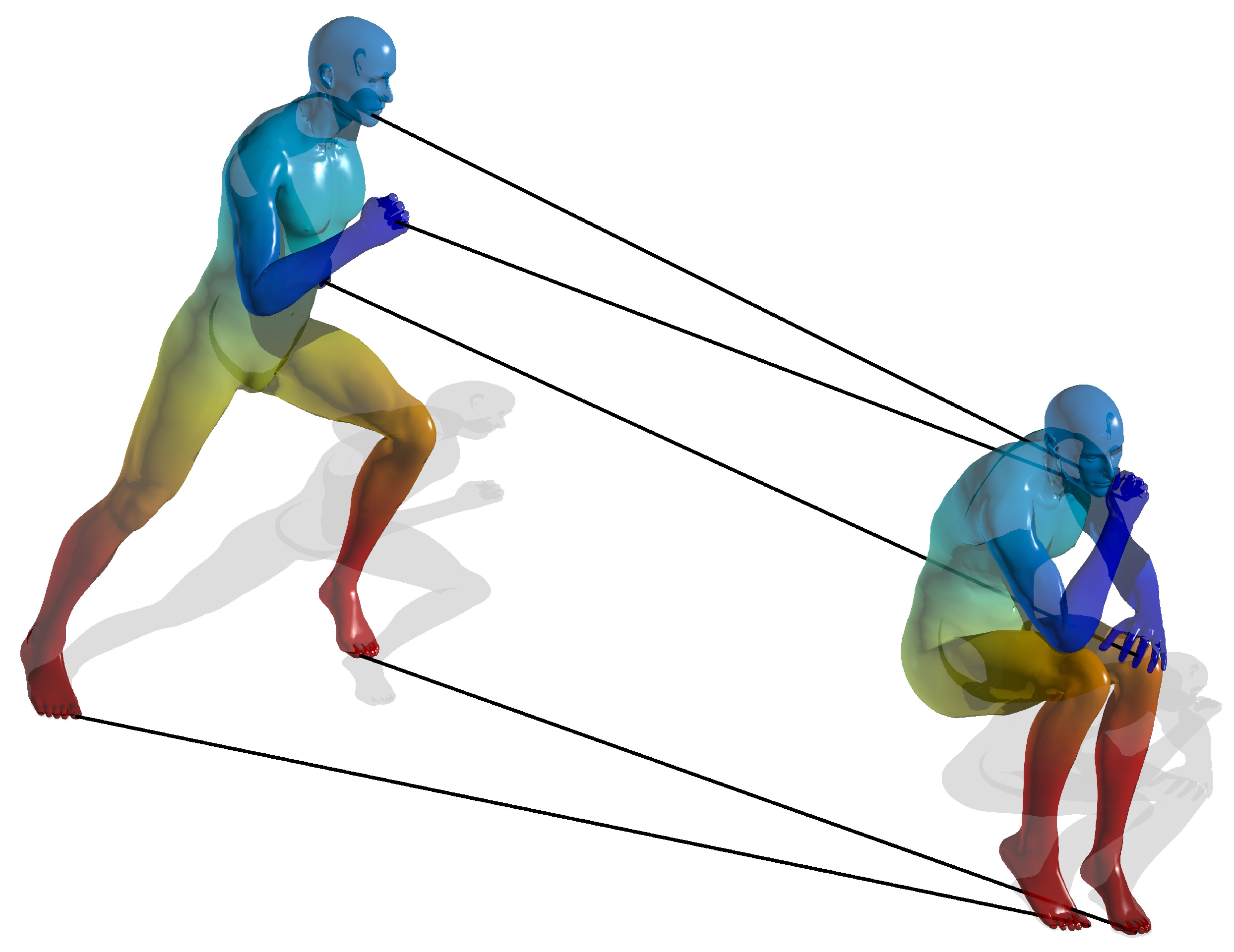
Figure 2, Figure 4 and Figure 6 show that the correspondences between feature points were found correctly. Notice that this approach was able to resolve the symmetries of the given shapes.

The algorithm was implemented in MATLAB. All of the experiments were executed on a 3.00 GHz Intel Core i7 machine with 32 GB of RAM. The runtime for matching the eigenfuctions for a typical pair of shapes from the TOSCA database is 1.5 s, excluding the calculation of the eigenfunctions.

We utilized these feature points to propagate correspondence to the whole shape. The signatures we used for this application were:

• The global point signature (GPS) kernel (Equation (A12)), propagating the correspondence of each feature point.
• The heat kernel signature (HKS) derivative (Equation (A11)), as before.

Figure 1. The eigenfunction matching of two nearly isometric shapes. Hot and cold colors represent positive and negative values, respectively. (Top) The first pose of a dog; (center) the second pose of a dog; (bottom) the second pose of a dog after the matching algorithm.

Figure 1. The eigenfunction matching of two nearly isometric shapes. Hot and cold colors represent positive and negative values, respectively. (Top) The first pose of a dog; (center) the second pose of a dog; (bottom) the second pose of a dog after the matching algorithm.

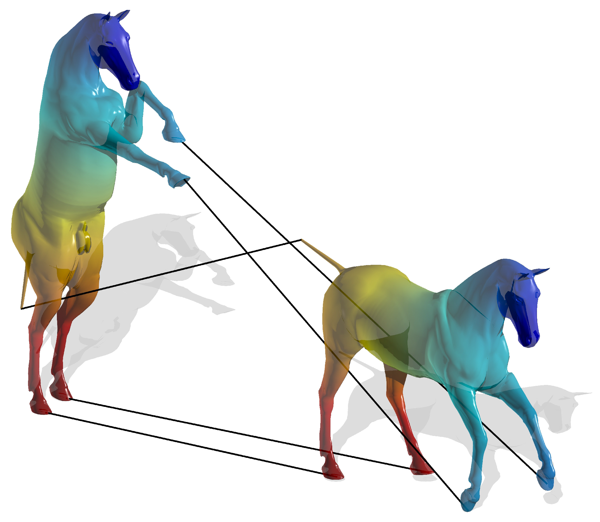
Figure 2. Feature point correspondence of two nearly isometric shapes of a horse.

Figure 2. Feature point correspondence of two nearly isometric shapes of a horse.

Figure 3. Eigenfunction matching of two nearly isometric shapes. Hot and cold colors represent positive and negative values, respectively. (Top) The first pose of a human; (center) the second pose of a human; (bottom) the second pose of a human after the matching algorithm.

Figure 3. Eigenfunction matching of two nearly isometric shapes. Hot and cold colors represent positive and negative values, respectively. (Top) The first pose of a human; (center) the second pose of a human; (bottom) the second pose of a human after the matching algorithm.

Figure 4. Feature point correspondence of two nearly isometric shapes of a horse.

Figure 4. Feature point correspondence of two nearly isometric shapes of a horse.

Figure 5. Eigenfunction matching of two nearly isometric shapes. Hot and cold colors represent positive and negative values, respectively. (Top) The first pose of a horse; (center) the second pose of a horse; (bottom) the second pose of a horse after the matching algorithm.

Figure 5. Eigenfunction matching of two nearly isometric shapes. Hot and cold colors represent positive and negative values, respectively. (Top) The first pose of a horse; (center) the second pose of a horse; (bottom) the second pose of a horse after the matching algorithm.

Figure 6. Feature point correspondence of two nearly isometric shapes of a horse.

Figure 6. Feature point correspondence of two nearly isometric shapes of a horse.

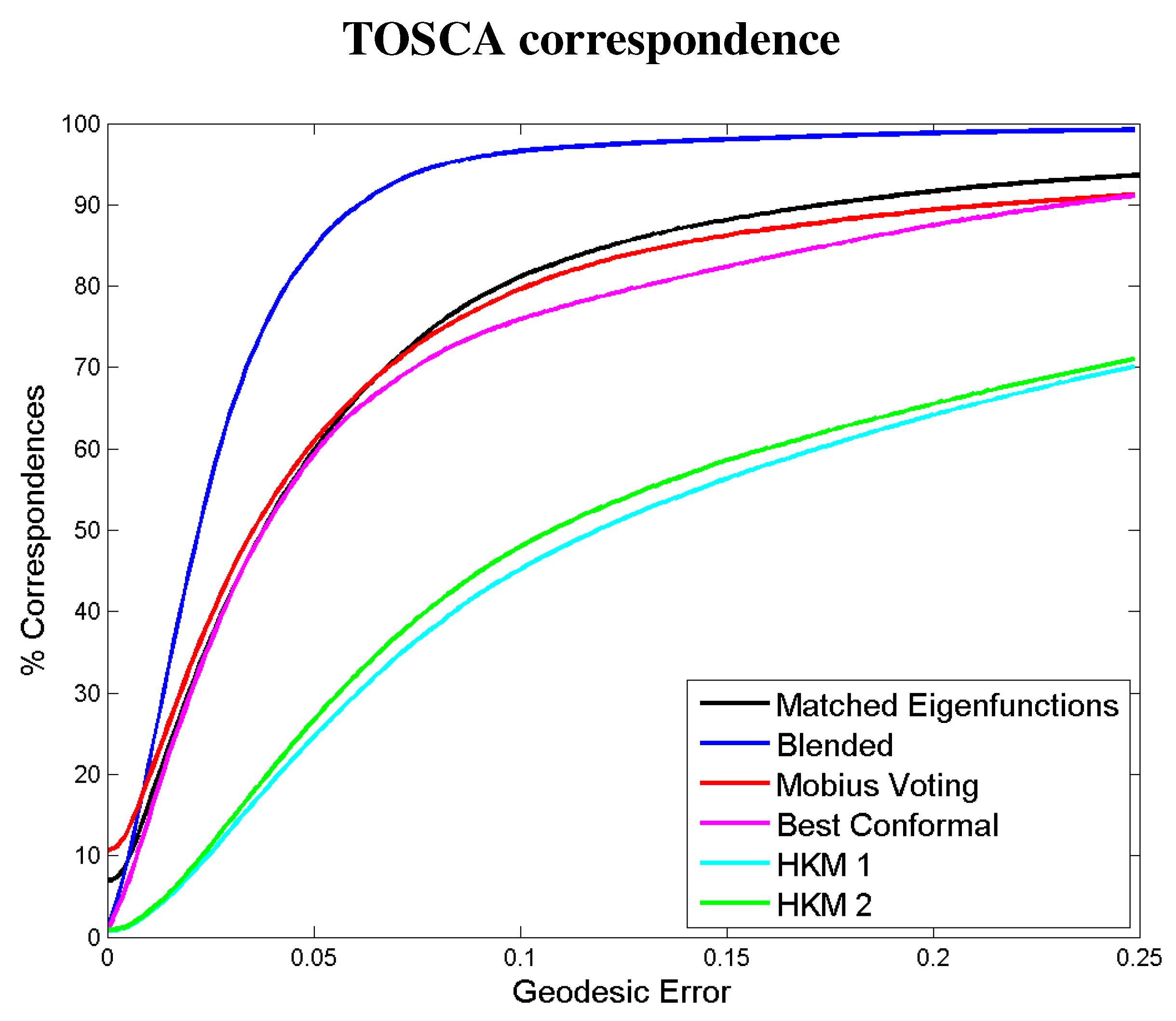
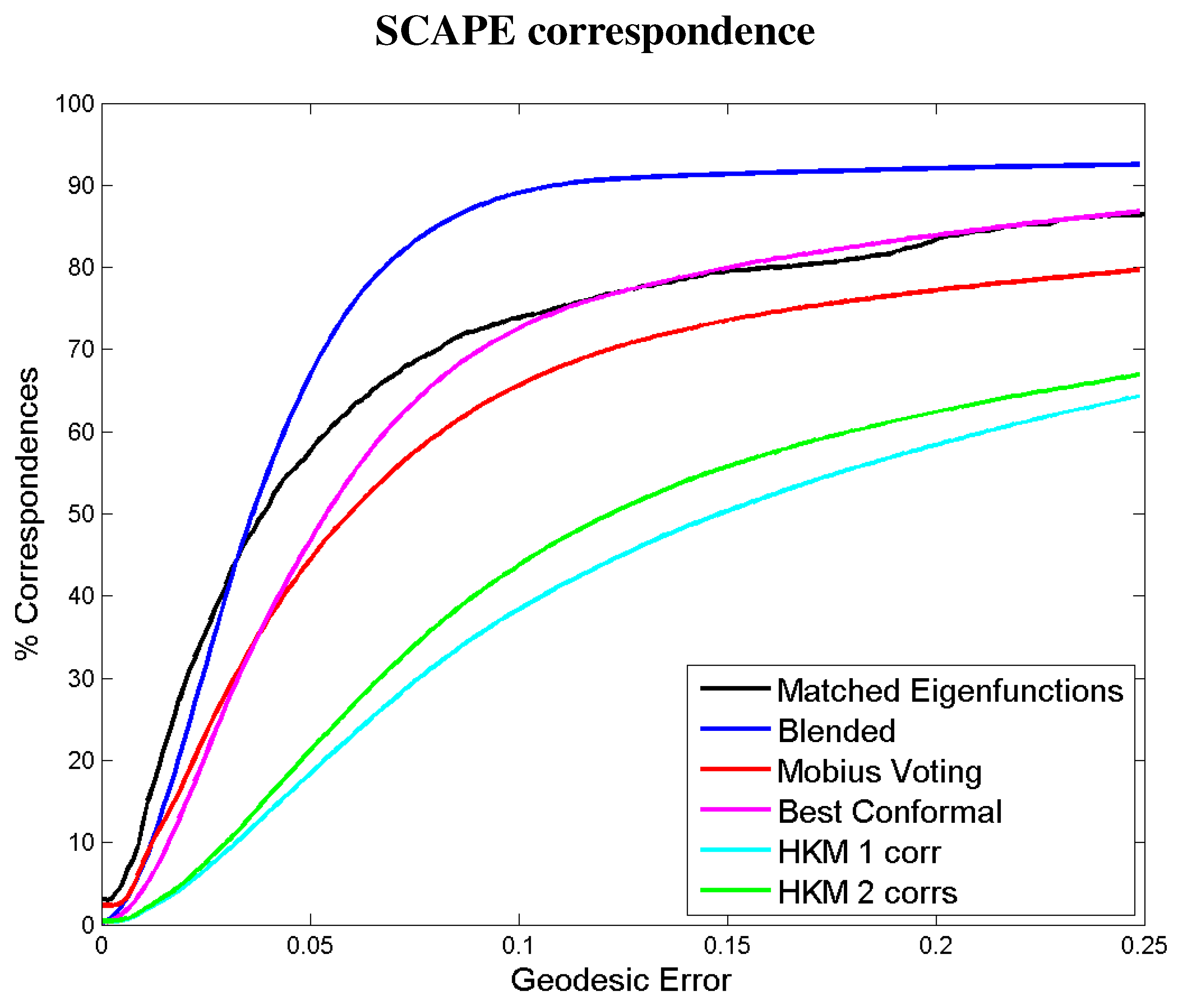
The correspondence method was applied to pairs of shapes represented by triangulated meshes from both the TOSCA and SCAPE databases [22,23]. The TOSCA dataset contains densely sampled synthetic human and animal surfaces, divided into several classes with given ground-truth point-to-point correspondences between the shapes within each class. The SCAPE dataset contains scans of real human bodies in different poses. We compare our work to several correspondence detection methods.

• Matched eigenfunctions: the method proposed in this paper.
• Blended: the method proposed by Kim et al. [24] that uses a weighted combination of isometric maps.
• Best conformal: the least-distortive conformal map roughly describes what is the best performance achieved by a single conformal map without blending.
• Möbius voting: the method proposed by Lipman et al. [25] counts votes on the conformal Möbius transformations.
• Heat kernel matching (HKM) with one correspondence: This method is based on matching features in a space of a heat kernel for a given source point, as described in [26]. A full map is constructed from a single correspondence, which is obtained by searching a correspondence that gives the most similar heat kernel maps. We use the results shown in [24].
• HKM with tow correspondences: in a non-isometric case, the previous method might obtain better results by using a second correspondence. The matching is then performed in the augmented feature space of two heat kernel maps [26]. We use the results shown in [24].

Note that all of the above methods, including the one we propose, can be followed by the post-processing iterative refinement algorithm [27]. The refinement procedure is based on the iterative closest point (ICP) method [28,29], applied in the spectral domain, and is known to improve the quality of other isometric shape matching methods.

Figure 7 and Figure 8 compare our correspondence framework with existing methods on the TOSCA benchmark and SCAPE, using the evaluation protocol proposed in [24]. The distortion curves describe the percentage of surface points falling within a relative geodesic distance from what is assumed to be their true locations. For each shape, the geodesic distance is normalized by the square root of the shape’s area. We see that out of the methods we compared, the proposed method is second best to the blended method, which is currently state-of-the-art.

Figure 7. Evaluation of the proposed correspondence framework applied to shapes from the TOSCA database, using the protocol of [24].

Figure 7. Evaluation of the proposed correspondence framework applied to shapes from the TOSCA database, using the protocol of [24].

Figure 8. Evaluation of the proposed correspondence framework applied to shapes from the SCAPE database, using the protocol of [24].

Figure 8. Evaluation of the proposed correspondence framework applied to shapes from the SCAPE database, using the protocol of [24].

4. Conclusions

The Laplace–Beltrami operator (LBO) provides us with a flat eigenspace in which surfaces could be represented as canonical forms in an isometric invariant manner. However, the order and directions (signs) of the axises in this Hilbert space do not have to correspond when two isometric surfaces are considered. In order to resolve such potential ambiguities, we resorted to high order statistics of the eigenfunctions of the LBO and their interaction with the surface normal. It appears that these cross moments allow for ordered directional matching of the components of corresponding eigenspaces. We demonstrated that resolving the sign and order correspondence allows for shape matching in various scenarios. In the future, we plan on extending the proposed framework to enable it to deal with more generic transformations, like the scale-invariant metric introduced by Aflalo et al. [30].

Acknowledgments We thank Anastasia Dubrovina for helpful discussions and suggestions during the progress of this work. This work has been supported by Grant Agreement No. 267414 of the European Community’s FP7-ERC program.

References

- Elad, A.; Kimmel, R. Pattern Analysis and Machine Intelligence. IEEE Trans. Bend. Invariant Signat. Surf. 2003, 25, 1285–1295. [Google Scholar]
- Kimmel, R.; Sethian, J.A. Computing geodesic paths on manifolds. Proc. Natl. Acad. Sci. USA 1998, 95, 8431–8435. [Google Scholar] [CrossRef] [PubMed]
- Bérard, P.; Besson, G.; Gallot, S. Embedding Riemannian manifolds by their heat kernel. Geom. Funct. Analy. GAFA 1994, 4, 373–398. [Google Scholar] [CrossRef]
- Hausdorff, F. Set Theory; American Mathematical Society: Providence, RI, USA, 1957; Volume 119. [Google Scholar]
- Coifman, R.R.; Lafon, S.; Lee, A.B.; Maggioni, M.; Nadler, B.; Warner, F.; Zucker, S.W. Geometric diffusions as a tool for harmonic analysis and structure definition of data: Diffusion maps. Proc. Natl. Acad. Sci. USA 2005, 102, 7426–7431. [Google Scholar] [CrossRef] [PubMed]
- Rustamov, R.M. Laplace–Beltrami eigenfunctions for deformation invariant shape representation. In Proceedings of the fifth Eurographics symposium on Geometry processing, Barcelona, Spain, 4–6 July 2007.
- Shapiro, L.S.; Michael, B.J. Feature-based correspondence: An eigenvector approach. Image Vis. Comput. 1992, 10, 283–288. [Google Scholar] [CrossRef]
- Jain, V.; Zhang, H.; van Kaick, O. Non-rigid spectral correspondence of triangle meshes. Int. J. Shape Model. 2007, 13, 101–124. [Google Scholar] [CrossRef]
- Umeyama, S. An eigendecomposition approach to weighted graph matching problems. IEEE Trans. Pattern Anal. Mach. Intell. 1988, 10, 695–703. [Google Scholar] [CrossRef]
- Mateus, D.; Cuzzolin, F.; Horaud, R.; Boyer, E. Articulated shape matching using locally linear embedding and orthogonal alignment. In Proceedings of the IEEE 11th International Conference (ICCV 2007), Rio de Janeiro, Brazil, 14–20 October 2007.
- Mateus, D.; Horaud, R.; Knossow, D.; Cuzzolin, F.; Boyer, E. Articulated shape matching using laplacian eigenfunctions and unsupervised point registration. In Proceedings of the IEEE Conference on Computer Vision and Pattern Recognition (CVPR 2008), Anchorage, AK, USA, 23–28 June 2008.
- Knossow, D.; Sharma, A.; Mateus, D.; Horaud, R. Inexact matching of large and sparse graphs using laplacian eigenvectors. Gr. Based Represent. Pattern Recognit. 2009, 5534, 144–153. [Google Scholar]
- Dubrovina, A.; Kimmel, R. Approximately isometric shape correspondence by matching pointwise spectral features and global geodesic structures. Adv. Adapt. Data Anal. 2011, 3, 203–228. [Google Scholar] [CrossRef]
- Kovnatsky, A.; Bronstein, A.M.; Bronstein, M.M.; Glashoff, K.; Kimmel, R. Coupled quasi-harmonic bases. Comput. Gr. Forum 2013, 32. [Google Scholar] [CrossRef]
- Pokrass, J.; Bronstein, A.M.; Bronstein, M.M.; Sprechmann, P.; Sapiro, G. Sparse Modeling of Intrinsic Correspondences. Eurogr. Comput. Gr. Forum 2013, 32. [Google Scholar] [CrossRef]
- Taubin, G. A signal processing approach to fair surface design. In Proceedings of the 22nd annual conference on Computer graphics and interactive techniques. (ACM), Los Angeles, CA, USA, 6–11 August 1995; pp. 351–358.
- Lévy, B. Laplace-Beltrami Eigenfunctions Towards an Algorithm That Understands Geometry. In Proceedings of the IEEE International Conference on Shape Modeling and Applications 2006, Washington, DC, USA, 14–16 June 2006.
- Kullback, S.; Leibler, R.A. On information and sufficiency. Ann. Math. Stat. 1951, 22, 79–86. [Google Scholar] [CrossRef]
- Lin, J. Divergence measures based on the Shannon entropy. IEEE Trans. Inf. Theory 1991, 37, 145–151. [Google Scholar] [CrossRef]
- Raviv, D.; Bronstein, A.M.; Bronstein, M.M.; Kimmel, R. Symmetries of non-rigid shapes. In IEEE 11th International Conference on Computer Vision (ICCV 2007), Rio de Janeiro, Brazil, 14–20 October 2007.
- Sun, J.; Ovsjanikov, M.; Guibas, L. A Concise and Provably Informative Multi-Scale Signature Based on Heat Diffusion. Comput. Gr. Forum. 2009, 28, 1383–1392. [Google Scholar] [CrossRef]
- Bronstein, A.M.; Bronstein, M.; Kimmel, R. Numerical Geometry of Non-Rigid Shapes; Springer: Berlin, Germany, 2008. [Google Scholar]
- Anguelov, D.; Srinivasan, P.; Pang, H.C.; Koller, D.; Thrun, S.; Davis, J. The correlated correspondence algorithm for unsupervised registration of nonrigid surfaces. Adv. Neural Inf. Process. Syst. 2005, 17, 33–40. [Google Scholar]
- Kim, V.G.; Lipman, Y.; Funkhouser, T. Blended intrinsic maps. ACM Trans. Gr. 2011, 30. [Google Scholar] [CrossRef]
- Lipman, Y.; Funkhouser, T. Möbius voting for surface correspondence. ACM Trans. Gr. 2009, 28. [Google Scholar] [CrossRef]
- Ovsjanikov, M.; Mérigot, Q.; Mémoli, F.; Guibas, L. One point isometric matching with the heat kernel. Comput. Gr. Forum 2010, 29, 1555–1564. [Google Scholar] [CrossRef]
- Ovsjanikov, M.; Ben-Chen, M.; Solomon, J.; Butscher, A.; Guibas, L. Functional maps: A flexible representation of maps between shapes. ACM Trans. Gr. 2012, 31. [Google Scholar] [CrossRef]
- Yang, C.; Medioni, G. Object modelling by registration of multiple range images. Image Vis. Comput. 1992, 10, 145–155. [Google Scholar]
- Besl, P.J.; McKay, N.D. Method for registration of 3-D shapes. In Robotics-DL Tentative; Ihe International Society for Optics and Photonics: Bellingham, WA, USA, 1992. [Google Scholar]
- Aflalo, Y.; Raviv, D.; Kimmel, R. Scale Invariant Geometry for Non-Rigid Shapes; Technical Report for Society for Industrial and Applied Mathematics: Philadelphia, PA, USA, 2011. [Google Scholar]
- Ulrich, P.; Strasse, D.J.; Konrad, P. Computing Discrete Minimal Surfaces and Their Conjugates. Exp. Math. 1993, 2, 15–36. [Google Scholar]
- Meyer, M.; Desbrun, M.; Schröder, P.; Barr, A.H. Discrete differential-geometry operators for triangulated 2-manifolds. Vis. Math. 2002, 3, 34–57. [Google Scholar]
© 2014 by the authors; licensee MDPI, Basel, Switzerland. This article is an open access article distributed under the terms and conditions of the Creative Commons Attribution license (http://creativecommons.org/licenses/by/3.0/).
Share and Cite
MDPI and ACS Style
Shtern, A.; Kimmel, R. Matching the LBO Eigenspace of Non-Rigid Shapes via High Order Statistics. Axioms 2014, 3, 300-319. https://doi.org/10.3390/axioms3030300
AMA Style
Shtern A, Kimmel R. Matching the LBO Eigenspace of Non-Rigid Shapes via High Order Statistics. Axioms. 2014; 3(3):300-319. https://doi.org/10.3390/axioms3030300
Chicago/Turabian StyleShtern, Alon, and Ron Kimmel. 2014. "Matching the LBO Eigenspace of Non-Rigid Shapes via High Order Statistics" Axioms 3, no. 3: 300-319. https://doi.org/10.3390/axioms3030300