A Comparative Study of Several Classical, Discrete Differential and Isogeometric Methods for Solving Poisson’s Equation on the Disk

Abstract

This paper outlines and qualitatively compares the implementations of seven different methods for solving Poisson’s equation on the disk. The methods include two classical finite elements, a cotan formula-based discrete differential geometry approach and four isogeometric constructions. The comparison reveals numerical convergence rates and, particularly for isogeometric constructions based on Catmull–Clark elements, the need to carefully choose quadrature formulas. The seven methods include two that are new to isogeometric analysis. Both new methods yield $O\left(h^3\right)$ convergence in the $L^2$ norm, also when points are included where $n\ne 4$ pieces meet. One construction is based on a polar, singular parameterization; the other is a $G^1$ tensor-product construction.

1. Introduction

In classical analysis, physical laws are described by a set of (partial) differential equations from which the qualitative behavior of physical systems is deduced. The differential operators used in these equations are continuous in the sense that they are based on infinitesimal change. To obtain quantitative information, one has to typically rely on computational methods. Computational methods may discretize the operator or discretize the underlying solution space of the equations. An alternative is the theory of discrete differential geometry (DDG), which starts with a discrete description and tries to preserve key properties of the underlying continuous systems in the form of important invariants.

This paper compares the convergence rates of the implementations of seven different approaches for solving Poisson’s equation on the disk. Besides the DDG approach [1,2], the comparison includes two classical $C^0$ and $C^1$ finite (Hsieh–Clough–Tocher) elements and four flavors of isogeometric analysis (IgA). IgA is a form of isoparametric analysis (see Section 3) using higher-order elements, such as tensor-product B-splines, both to describe the domain and the approximate solution of a partial differential equation. IgA currently has some limitations, foremost being the sub-optimal numerical convergence rate, where the spline elements are not laid out regularly, i.e., where they are not arranged as quad-grids or a hierarchical refinement thereof [3,4,5,6]. Choosing Poisson’s equation on the disk as the model problem forces the introduction of irregular mesh points.

The paper’s contributions to the state-of-the-art are:

• a qualitative comparison between classical finite elements, a DDG approach and four isogeometric constructions;
• an investigation of quadrature formulas for subdivision IgA finite elements;
• implementation of an IgA method for $C^1$ functions on complex domains that is based on $G^1$ constructions and yields $O\left(h^3\right)$ convergence, also at irregular points; this improved convergence is confirmed for an L-shaped domain and for an elastic plate with a circular hole;
• implementation of an IgA method with singular parameterization at irregular points that yields $O\left(h^3\right)$ convergence also at irregular points.

Overview

Section 2 gives an overview of the two classical finite element spaces and the canonical DDG approach to Poisson’s equation. Section 3 describes four partly new approaches to constructing $C^1$ functions over complex domains by using singular, respectively, geometrically continuous splines. Section 4 succinctly reviews the classical variational framework for the Poisson equation. Section 5 compares numerical convergence rates, as summarized in Figure 10.

2. Classical Finite and DDG Elements

This section briefly reviews standard non-linear finite elements and the cotan formula-based DDG approach.

2.1. $C^0$ Quadratic Triangular Elements

Also known as the linear strain triangle (LST) or Veubeke triangle, the $C^0$ quadratic triangular element was developed by B. M. Fraeijs de Veubeke [7]. The six degrees of freedom of a polynomial of a total degree two in two variables can be expressed as the coefficients, $c_{ijk}$, of the polynomial in total degree Bernstein-Bézier form (BB-form; see, e.g., [8]):

$$b^{▵}(u,v):=\sum _{i+j+k=2}{c}_{ijk}\frac{2!}{i!j!k!}{(1-u-v)}^i{u}^j{v}^k,i,j,k\in {\mathbb{N}}_0,0\le u,v\le 1,0\le u+v\le 1$$

(1)

Figure 1 shows the two types of $C^0$ quadratic elements, one associated with a vertex, the other with the mid-edge of a triangle.

Figure 1. $C^0$ quadratic basis functions. (a,c) top view with height scale. (a) Nodal basis function; (b) BB-piece of (a); (c) mid-edge basis function; (d) BB-piece of (c).

Figure 1. $C^0$ quadratic basis functions. (a,c) top view with height scale. (a) Nodal basis function; (b) BB-piece of (a); (c) mid-edge basis function; (d) BB-piece of (c).

2.2. Hsieh–Clough–Tocher Elements

The Hsieh–Clough–Tocher (HCT) element is a classical $C^1$ finite element (see, e.g., [9]). The HCT-element is piecewise polynomial of degree three. It is constructed over a triangle domain split into three sub-triangles by connecting the vertices to the barycenter. The resulting three-piece $C^1$ function has 12 degrees of freedom, which one may choose as the value and first derivatives at each vertex, plus normal derivatives on the midpoint of each edge. The twelve basis functions overlapping a triangle are constructed by setting one of the degrees of freedom to one and all others to zero. This is most conveniently expressed in total-degree three Bernstein–Bézier basis functions $b_k^{▵}$. We associate three basis functions $b_{3i+j}^{▵},j=0,1,2$ with the value and the partial derivatives at each vertex $v_i,i=1\dots \overline{n}$ and one basis function, $b_{3\overline{n}+k}^{▵}$, with each edge, $e_k$. The functions $b_{3i+j}^{▵}$ have support on the triangles with common vertex $v_i$, and the functions $b_{3\overline{n}+k}^{▵}$ have support on the triangles sharing $e_k$ (see Figure 2).

There are other methods of building smooth finite elements on split triangles, for example the Powell–Sabin construction [10]. The general theory is presented by Lai and Schumaker [11]. Recently, these classical elements have been applied to IgA, for example [12] or [13].

Figure 2. Hsieh–Clough–Tocher (HCT) basis functions (top view with height scale). (a) $b_{3i}^{▵}$: nodal basis function; (b) $b_{3i+1}^{▵}$: x-derivative basis function; (c) $b_{3N+k}^{▵}$: mid-edge normal derivative function.

Figure 2. Hsieh–Clough–Tocher (HCT) basis functions (top view with height scale). (a) $b_{3i}^{▵}$: nodal basis function; (b) $b_{3i+1}^{▵}$: x-derivative basis function; (c) $b_{3N+k}^{▵}$: mid-edge normal derivative function.

2.3. The Discrete Differential Geometry Approach

The theory of discrete differential geometry (DDG), starts with a discrete formulation that strives to preserve key properties of the underlying continuous systems in the form of important invariants. An example of a DDG operator is the cotangent formula for modeling the Laplace–Beltrami operator (see, e.g., Pinkall and Polthier [1]). In applications, DDG generalizes the principles underlying the continuous operator to make methods directly applicable to the data and to improve robustness over just discretizing the continuous operators.

The cotangent formula discretizes the Laplace–Beltrami operator on a triangular mesh. Among the desirable properties for discrete Laplacians enumerated in [14], we are mainly concerned with convergence in the sense that the discretization solves, in the limit under refinement, the PDEs correctly. In [15], Desbrun et al. (see also [16]) define the cotan operator, for a function, f, at a vertex, $v_i$, of a triangular mesh, M, as:

$$\begin{array}{c}\hfill {\Delta }_{M}f\left(v_i\right):={\displaystyle \frac{3}{\mathcal{A}\left(v\right)}}\sum _{j\in {\mathcal{N}}_1\left(i\right)}{\displaystyle \frac{cot{\alpha }_{ij}+cot{\beta }_{ij}}{2}}[f\left(v_j\right)-f\left(v_i\right)]\end{array}$$

(2)

where $\mathcal{A}\left(v\right)$ is the area of all the triangles of the one-ring neighbors of $v_i$, ${\mathcal{N}}_1\left(i\right)$ is the set of the vertex indices of one-ring neighbors and ${\alpha }_{ij}$ and ${\beta }_{ij}$ are the two angles opposite to the edge in the two triangles having the edge, $e_{ij}$, in common (see Figure 3a). In [17], G. Xu proved that Equation (2) converges to second order to the continuous operator if each $v_i$ has valence six and $v_i$ and $v_j$ lie on a sufficiently smooth surface. More general convergence guarantees appeared in [18]. In [19], K. Crane et al. derive the cotangent formula from linear finite element methods, whose a basis function is shown in Figure 3b and, alternatively, via discrete exterior calculus. For higher order PDEs, such as thin shell simulation [20], energy methods have been adopted.

DDG has found use in computer graphics and computing for architectural geometry [20,21] and is at the heart of discrete exterior calculus (see, e.g., [22]). Formula (2) has been successfully applied to geometry processing and simulation on mesh models (see, e.g., [23]).

Figure 3. Discrete differential geometry (DDG) notation and linear functions. (a) Notation of Equation (2); (b) top view of the linear “hat” function.

Figure 3. Discrete differential geometry (DDG) notation and linear functions. (a) Notation of Equation (2); (b) top view of the linear “hat” function.

3. The Isogeometric Approach

The next four methods model both the physical domain, Ω (the disk), and the PDE discretization space by tensor-product spline-like functions:

$$\sum _i{c}_i{b}_i^{\square }(s,t)=\sum _{j,k}{c}_{jk}{N}_j\left(s\right)N_k\left(t\right)$$

(3)

where $b_i^{\square }:=N_j{N}_k$ is the i-th tensor-product basis function defined on a standard domain, such as the unit square, T. We will use polynomial splines, except at the domain boundary, where the circle is exactly expressed in rational Bernstein–Bézier form.

The four methods will be used in the framework of IgA. IgA is a special case of the classical isoparametric analysis. The term, isogeometric analysis (IgA) was coined by T. Hughes et al. [24] in an effort to eliminate the representation gap between computer aided design and engineering analysis. In particular, IgA proponents have advocated the B-spline representation [25], both for modeling the geometry of Ω and for presenting the bases, $b_i^{\square }$, of the differential geometric analysis.

To define basis functions $b_i$ on Ω, one first represents the physical domain as the image of copies of T under the spline maps, ${\mathbf{x}}_{\alpha }:T\to \Omega$ (cf. Figure 4a):

$$\begin{array}{c}\hfill \Omega :={\cup }_{\alpha =1}^n{\mathbf{x}}_{\alpha }\left(T\right)T⊊{\mathbb{R}}^2\end{array}$$

(4)

Then, the space of functions on $\Omega \left(T\right)$ are obtained by composing test functions, also defined on T, with the inverse of ${\mathbf{x}}_{\alpha }$ (see Figure 4b). In IgA, we use test functions ${\left(b_i^{\square }\right)}_{\alpha }:T\to \mathbb{R}$, where ${\left(b_i^{\square }\right)}_{\alpha }$ is the part of the i-th basis function, $b_i^{\square }$, on the domain piece defined by ${\Omega }_{\alpha }$. That is, the test functions are drawn from the same space as ${\mathbf{x}}_{\alpha }$. Then, the discretization space on Ω is the span of the functions (see Figure 4b).

$$\begin{array}{c}\hfill b_i{|}_{{\mathbf{x}}_{\alpha }\left(T\right)}:={\left(b_i^{\square }\right)}_{\alpha }\circ {\mathbf{x}}_{\alpha }^{-1},1\le \alpha \le n\end{array}$$

(5)

A main open challenge of IgA are extraordinary points, where more or less than four tensor-product patches join. (The analogue in the case of three-sided patches is to have more or less than six elements meet at a point.) Such points occur for topological reasons, by Euler’s count, and are often inserted to better adjust the mesh to the local geometry. This is illustrated in Figure 5b, where a central $n=5$-valent (five-neighbor) point is surrounded by n three-valent points. Without a sophisticated treatment of extraordinary points, the advantage of high-order methods in IgA may be nullified by slow convergence near these points. There is an ongoing, vigorous discussion of the proper choice of refinement space for hierarchical adaptive modeling [3,4,5,6], but this does not address the modeling at extraordinary points.

Figure 4. A basis function, $b_i$, is the composition of the basis function, $b_i^{\square }$, on the tensor-product parameter domain, T, and the inverse of the geometry mapping, $\mathbf{x}$. (a) The union of $4\times 4$ domains T and its image, Ω, under $4\times 4$ maps ${\mathbf{x}}_{\alpha }$. (a) (left) Union domains T and (right) the physical domain Ω; (b) basis function $b_i^{\square }$ on T, respectively on Ω.

Figure 4. A basis function, $b_i$, is the composition of the basis function, $b_i^{\square }$, on the tensor-product parameter domain, T, and the inverse of the geometry mapping, $\mathbf{x}$. (a) The union of $4\times 4$ domains T and its image, Ω, under $4\times 4$ maps ${\mathbf{x}}_{\alpha }$. (a) (left) Union domains T and (right) the physical domain Ω; (b) basis function $b_i^{\square }$ on T, respectively on Ω.

Figure 5. The non-smooth $C^0$ bi-3 basis function: (a, left) A quad mesh of points associated with B-spline-like functions, for $n=5$. (a, right) The coefficients of the patches in tensor-product BB-form defined by the $C^2$ extension of the regular spline complex towards the extraordinary point (see [29]). Note the $n=5$ points of valence three surrounding the central n-valent point. (a) Control net and $C^2$ extension in BB-form; (b) $C^0$ bi-3 basis function.

Figure 5. The non-smooth $C^0$ bi-3 basis function: (a, left) A quad mesh of points associated with B-spline-like functions, for $n=5$. (a, right) The coefficients of the patches in tensor-product BB-form defined by the $C^2$ extension of the regular spline complex towards the extraordinary point (see [29]). Note the $n=5$ points of valence three surrounding the central n-valent point. (a) Control net and $C^2$ extension in BB-form; (b) $C^0$ bi-3 basis function.

Our four constructions represent alternative approaches to deal with the extraordinary points. We focus on higher-order spline-like representations that mimic bi-cubic (bi-3) tensor-product splines. Our first choice is the space of polynomials of degree bi-3 that are $C^2$, except near the extraordinary points, where they are only continuous. We will see that this simple space has good convergence except at the extraordinary point. This flaw motivates and makes the case for our other three constructions. Our second construction leverages Catmull–Clark subdivision. This is inspired by the seminal work of F. Cirak et al. [26,27], who used subdivision surface functions over triangulations for thin shell analysis. The challenge, not emphasized in the original work, is the choice of integration rules (see Section 5.1). Our remaining constructions come from geometric modeling and are new to IgA. The third construction leverages everywhere $G^1$ functions (that are $C^1$ when considered over the physical domain). Here, $G^1$ refers to geometric continuity, i.e., the matching of derivatives after the reparametrization of one or both of the adjacent function pieces (see [28]). Just as for Catmull–Clark subdivision, the space of generating functions consists of $C^2$ polynomial splines of degree bi-3 away from extraordinary points. Finally, we introduce $C^1$ functions with a polar layout, i.e., with a central pole or singularity. The last three constructions allow us to address high-order PDEs, such as the Kirchhoff–Love shell model or buckling analysis, which are not the focus of the present exposition.

3.1. Bi-3 Elements That Are $C^0$ at Extraordinary Points

A single Catmull–Clark refinement step converts any mesh into a mesh that consists of only quadrilateral facets, short quads. When all four vertices of a quad have valence four, i.e., are surrounded by four quads, then each $3\times 3$ submesh can be interpreted as the control net of one bi-3 (bi-cubic) polynomial piece in tensor-product B-spline representation. A regular grid pattern of quads then defines a bi-3 $C^2$ tensor-product spline.

At extraordinary points, this interpretation of the quad mesh breaks down. Assuming that extraordinary points are isolated, in the sense that no two extraordinary points share a quad, we can still construct a bi-3 $C^2$ tensor-product spline complex with “holes”, where $n\ne 4$ quads meet. A simple way to complete the spline complex is to extend the existing spline patches, $C^2$, into the holes, as n patches in bi-3 tensor-product BB-form (see Figure 5a, right). These patches are defined up to just one BB-coefficient, corresponding to the position at the center of the hole and common to all n patches. This coefficient is trivially set to the average of the surrounding coefficients. The result is bi-3 elements that form a standard $C^2$ bi-3 spline complex away from the extraordinary pointand that join $C^0$ at the extraordinary point (see Figure 5b).

3.2. Catmull–Clark Elements

Subdivision splines are piecewise polynomial splines with singularities at the extraordinary points [30]. The neighborhood of an extraordinary point is an infinite sequence of nested spline rings (where “ring” indicates the connectivity, not an algebraic ring). Subdivision splines have been used for finite element analysis well before the advent of IgA (see [26]), but did not receive the attention from the engineering community that IgA is currently generating. A more complicated framework for adaptive simulation with subdivision splines was introduced by E. Grinspun et al. in [31]. Subdivision-based functions for IgA on solid models were presented in [32,33]. The Catmull–Clark subdivision has been used in [34], the similar bi-2 spline-based Doo-Sabin subdivision in [35] and Loop’s subdivision in [36], for large deformation and anisotropic growth.

Among a myriad of subdivision schemes, Catmull–Clark dominates in industrial implementations. The Catmull–Clark subdivision refines a mesh by binary split in each direction (see Figure 6). The basis function associated with a vertex not on the boundary has support on two-ring neighbors. (For spline surfaces with a boundary, we apply “natural end conditions”, i.e., we do not evaluate under-defined outer quadrilaterals, after extrapolating the existing mesh.) Recently, Barendrecht performed experiments of the numerical convergence of IgA with Catmull–Clark surfaces and observed poor convergence near extraordinary points [37]. He conjectured that this is due to the well-known unbounded Gaussian curvature of the Catmull–Clark subdivision at these points. Based on our experiments in Section 5, Table 1, we think that the poor numerical convergence can be the result of of applying Gauss quadrature rules with respect to the original quads, rather than choosing quadrature points for each sub-polynomial of sufficiently many levels of refinement (see Figure 6a,b).

Figure 6. Catmull–Clark elements. (a) Refinement Level 3; (b) refinement Level 7; (c) a Catmull–Clark subdivision function.

Figure 6. Catmull–Clark elements. (a) Refinement Level 3; (b) refinement Level 7; (c) a Catmull–Clark subdivision function.

Table 1. Error (scaled by ${10}^{-5}$) of the computed solution of Poisson’s equation by Catmull–Clark subdivision on Disk 1 (see Figure Figure 6), for different levels of subdivision when applying the Gauss quadrature. The subdivision is localized to not refine the overall mesh.

Depth	$L^2$	$L^{\infty }$
3	893.063	476.26
5	100.44	81.193
7	70.395	47.004
9	70.073	43.992

Table 1. Error (scaled by ${10}^{-5}$) of the computed solution of Poisson’s equation by Catmull–Clark subdivision on Disk 1 (see Figure Figure 6), for different levels of subdivision when applying the Gauss quadrature. The subdivision is localized to not refine the overall mesh.

Depth	$L^2$	$L^{\infty }$
3	893.063	476.26
5	100.44	81.193
7	70.395	47.004
9	70.073	43.992

3.3. Higher-Order $G^1$ Elements

A technique from the applied mathematics area of geometric design allows the gluing together of function pieces with “geometric continuity”. The result is a $C^k$ manifold. The designation, $G^k$, is used to emphasize that derivatives of adjacent patches match only after reparametrization [28]. Geometric continuity then allows smoothly join $n\ne 4$ tensor-product pieces (often called patches) in the sense of parametric surfaces. Composition of a $G^1$ construction with the inverse of a $G^1$ construction that share the same reparametrization yields a $C^1$ function. There are many $G^1$ constructions in the literature. Some naturally complete a bi-3 $C^2$ tensor-product spline complex with bi-3 patches to a $G^1$ structure. To avoid splitting quadrilateral domains, we chose [38], a simplified version of [29] that deploys n bi-5 patches at the extraordinary point. The corresponding basis functions are shown in Figure 7. The resulting $G^1$ elements are $C^2$ at the extraordinary point. The additional smoothness at the extraordinary points guarantees high polynomial reproduction and, hence, high numerical convergence also at the extraordinary points.

Figure 7. $G^1$ element at an extraordinary point. (a) Two $G^1$ bi-3/bi-5 basis functions; (b) $G^1$ bi-3/bi-5 basis function with onepatch in BB-form lifted up.

Figure 7. $G^1$ element at an extraordinary point. (a) Two $G^1$ bi-3/bi-5 basis functions; (b) $G^1$ bi-3/bi-5 basis function with onepatch in BB-form lifted up.

3.4. Polar $C^1$ Elements

The polar parametric surface construction of [39] provides a simple element that is smooth and particularly well-behaved at points where many surfaces join in a triangle fan at the center of the disk (see Figure 8). To match the tensor-product standard, the triangle of the fan can be interpreted as quadrilaterals that have one edge collapsed. Analogous to the $G^1$ edges in the previous construction, the central singularity is no cause for concern for the shape. Note that this observation matches the recent results of Takacs and Jüttler [40], who analyze singularities at domain boundaries, where the test functions by themselves are not well-defined.

Figure 8. Polar elements for polar configurations. (a) Modeling with $C^1$ polar functions; (b) a $C^1$ polar basis function.

Figure 8. Polar elements for polar configurations. (a) Modeling with $C^1$ polar functions; (b) a $C^1$ polar basis function.

4. Solving the Poisson Equation

We are solving Poisson’s equation on the domain, Ω, subject to zero boundary conditions on the boundary, $\partial \Omega$, of Ω:

$$\begin{array}{c}\hfill -\Delta u=f,u(\partial \Omega )=0\end{array}$$

(6)

The DDG method discretizes this formulation directly as $-{\Delta }_{M}u=f$, where the operator, ${\Delta }_M$, has been defined in Equation (2).

For all six methods other than DDG, we solve the equation numerically by considering its weak form: find $u\in H_0^1$, such that for all $v\in H_0^1$:

$$\begin{array}{cc}\hfill {\int }_{\Omega }\nabla u·\nabla vd\Omega & ={\int }_{\Omega }fvd\Omega \hfill \end{array}$$

(7)

We seek an approximate solution in terms of the generating functions $b_i:\Omega \to \mathbb{R}$ defined in Equation (5) by determining the coefficients, $c_i\in \mathbb{R}$, in:

$$\begin{array}{c}\hfill u_h:=\sum _1^N{c}_i{b}_i\end{array}$$

(8)

Using Galerkin’s method, we set $v=b_i$ in Equation (7) and obtain the constraints:

$$\begin{array}{cc}\hfill {\int }_{\Omega }\nabla \left(\sum _1^N{c}_j{b}_j\right)·\nabla b_{i}d\Omega & ={\int }_{\Omega }f{b}_{i}d\Omega \hfill \end{array}$$

(7*)

This yields a system of linear equations:

$$\begin{array}{c}\hfill K\mathbf{c}=\mathbf{f},\text{where}{K}_{ij}:={\int }_{\Omega }\nabla b_i·\nabla b_{j}d\Omega ,\text{and}{\mathbf{f}}_i:={\int }_{\Omega }f{b}_{i}d\Omega \end{array}$$

(9)

and the vector of unknown coefficients is $\mathbf{c}:={[c_1,\cdots ,c_n]}^{\mathtt{t}}$.

For all isogeometric methods, we define the physical domain, Ω, as in Equation (4) and write the integrals in Equation (9) as a sum of integrals restricted to some ${\mathbf{x}}_{\alpha }\left(T\right)$. Using Equation (5) and dropping the subscript, α, we can, by the change of variables, express the local integrals with respect to each parameter domain, T, as:

$$\begin{array}{cc}\hfill K_{ij}& ={\int }_{\mathbf{x}\left(T\right)}\nabla (b_i^{\square }\circ {\mathbf{x}}^{-1})·\nabla (b_j^{\square }\circ {\mathbf{x}}^{-1})d\Omega ={\int }_T\left(J^{-1}\nabla b_i^{\square }\right)·\left(J^{-1}\nabla b_j^{\square }\right)|detJ|dT\hfill \\ & ={\int }_T{\left(\nabla b_i^{\square }\right)}^{\mathtt{t}}{\left[J^{-1}\right]}^{\mathtt{t}}{J}^{-1}\left(\nabla b_j^{\square }\right)|detJ|dT\hfill \end{array}$$

where J is the transpose of the Jacobian of the mapping $\mathbf{x}:(s,t)\in T\to {\left[x(s,v)y(s,v)\right]}^{\mathtt{t}}$. For implementation, we collect:

$$\begin{array}{cc}\hfill J:=\left[\begin{array}{cc}{x}_s& y_s\\ x_t& y_t\end{array}\right],detJ& =x_s{y}_t-x_t{y}_s,J^{-1}={\displaystyle \frac{1}{detJ}}\left[\begin{array}{cc}{y}_t& -y_s\\ -x_t& x_s\end{array}\right]\hfill \end{array}$$

(10)

$$\begin{array}{cc}\hfill {}^{-1}{]}^{\mathtt{t}}{J}^{-1}|detJ|& ={\displaystyle \frac{1}{|detJ|}}\left[\begin{array}{cc}{x}_t^2+y_t^2& -x_s{x}_t-y_s{y}_t\\ -x_s{x}_t-y_s{y}_t& x_s^2+y_s^2\end{array}\right]\hfill \end{array}$$

(11)

Similarly, for the right-hand side term,

$$\begin{array}{c}\hfill {\int }_{\Omega }f{b}_{i}d\Omega ={\int }_T(f\circ \mathbf{x})b_i^{\square }|detJ|dT\end{array}$$

(12)

5. Numerical Results and Comparison

Before we compare the convergence rates of the methods for Poisson’s equation on the disk, we need to look in more detail at the quadrature rules that are used for Catmull–Clark functions in the IgA setting to compute Equations (10) and (12).

5.1. Correct Gauss Quadrature for Catmull–Clark Subdivision

The p-point Gaussian quadrature rule is known to exactly calculate the integral of polynomials of degree up to $2p-1$. For piece-wise polynomials, Gaussian quadrature only gives approximate results. Table 1 shows that in order to obtain good integration results at irregular points, one needs to apply exact Gauss quadrature on many subdivision layers to obtain convergence. We found that subdivision of depth seven was necessary for results to stabilize. A more principled approach is to take advantage of the recursive nature of subdivision and compute the quadrature rules via eigendecomposition, as in Halstead et al. in ([41], Appendix B).

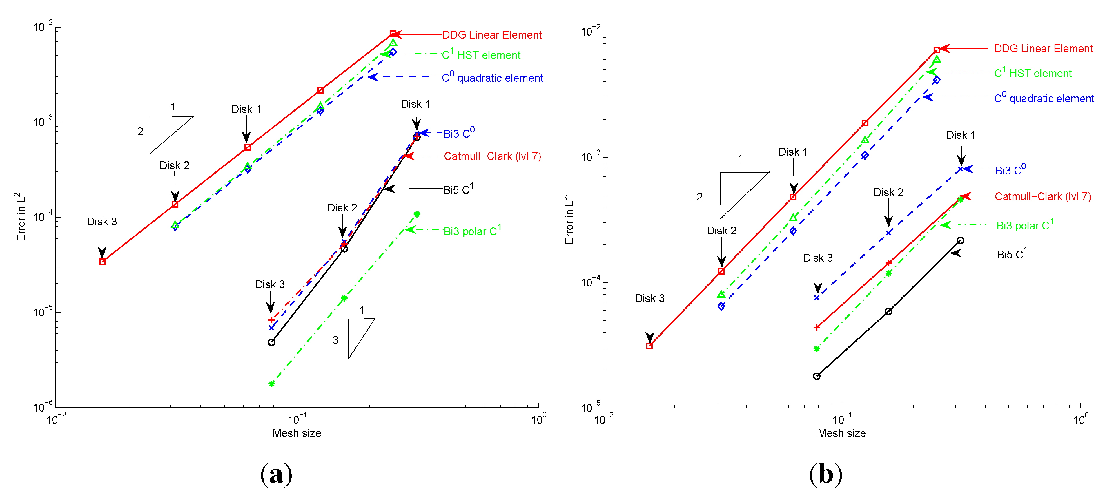
5.2. Convergence Rates

Figure 9 shows the three types of meshes that one might naturally associate with the methods. For $C^0$ quadratic, HCT and DDG elements, we optimized the aspect ratio of the triangles to guarantee numerical stability. These elements are non-conforming while the iso-geometric elements reproduce the boundary circle exactly. For bi-3 $C^0$, Catmull–Clark and $G^1$ bi-3/bi-5 elements, we chose a central extraordinary point with valence $n=5$, surrounded by n satellites of valence three. Other n can be tested or the singularities can be distributed to the boundary, as in Takacs and Jüttler’s approach [40]. Finally, the polar configuration is natural for the polar $C^1$ elements. The convergence of polar elements is remarkably unaffected by the valence of the central point. We choose $f:=1$ in Equation (6). Then, the exact solution is $u:=(1-x^2-y^2)/4$, and we can display the exact error.

Figure 10 confirms at least an $O\left(h^2\right)$ convergence for all higher-order methods, as well as for DDG. The graphs are in log-scale with smaller mesh spacing displayed to the left. That is, the entries to the left correspond to more elements. Figure 10 displays $O\left(h^3\right)$ $L^2$-norm convergence of the isogeometric approaches. The spread factor between the polar and the other three methods is five. That is, in the $L^2$ sense, the easily implemented $C^1$ polar isogeometric approach (that is natural for the disk) is superior. Remarkably, though, the more general $G^1$ construction excels in minimizing the $L^{\infty }$ norm. The spread in the error between the four $O\left(h^3\right)$-convergent methods is more than a factor of eight.

The higher $L^{\infty }$ error of Catmull–Clark elements (Figure 11a) and $C^0$ bi-3 elements (Figure 11c) is concentrated at the central point, as large spikes. This is to be expected, since neither method reproduces all quadratic expansions at the central point, a fact that is also reflected in their lack of $C^1$, respectively $C^2$ smoothness at the central point.

5.3. Complexity

We do not compare execution times, since implementation details, such as memory management on the GPU, pre-tabulation of basis functions or sparsity (taking advantage of finite support), etc., strongly influence the performance. However, we can state the size of the matrix, $\mathbf{K}$, in Equation (9) for the IgA methods. For Disk 1, the mesh (Figure 9e) used by bi-3 $C^0$, Catmull–Clark and $G^1$ bi-3/bi-5 elements $\mathbf{K}$ is a matrix of size $151\times 151$ for 120 patches. For Disk 1, the mesh (Figure 9f) used by $C^1$ polar elements $\mathbf{K}$ is a matrix of size $101\times 101$ for 80 patches. The relative times for solving Equation (9) by our unoptimized implementations showed a ratio of roughly 4:6:8:26 for $C^1$ polar, bi-3 $C^0$, $G^1$ bi-3/bi-5 and Catmull–Clark elements, respectively. We surmise that, in the natural disk setting, $C^1$ polar elements can achieve good results with fewer elements and fast computation. Remarkably, the quality of the polar method does not depend on the valence of the center point: the polar method’s $L^2$ error decreases with order of $O\left(h^3\right)$, even though the valence of the center point is doubled with each refinement step.

The three non-IgA-methods, and the DDG method in particular, have lower memory requirements. This allowed us to add very fine meshes for the comparison in Figure 10. For Disk 3, the mesh of type Figure 9d has 6,144 triangles, and 3,169, 12,481 and 18,819 degrees of freedom for DDG, $C^0$ elements and HCT elements, respectively. We observed solution times with a ratio of 2:10:37, making DDG attractive in comparison to the classical HCT elements.

Figure 9. Three types of meshes specific to each of the three classes of methods. (d) $C^0$ quadratic, HCT, DDG elements: 384, $384\times 4$, $384\times 16$ elements; (e) bi-3 $C^0$, Catmull–Clark and $G^1$ bi-3/bi-5 elements: 120, $120\times 4$, $120\times 16$ elements; (f) polar $C^1$ elements: 100, $100\times 4$, $100\times 16$ elements. Columns a, b, c correspond to refinement by halving h, hence quadrupling the number of elements, i.e. to (a) Disk 1; (b) Disk 2; (c) Disk 3;

Figure 9. Three types of meshes specific to each of the three classes of methods. (d) $C^0$ quadratic, HCT, DDG elements: 384, $384\times 4$, $384\times 16$ elements; (e) bi-3 $C^0$, Catmull–Clark and $G^1$ bi-3/bi-5 elements: 120, $120\times 4$, $120\times 16$ elements; (f) polar $C^1$ elements: 100, $100\times 4$, $100\times 16$ elements. Columns a, b, c correspond to refinement by halving h, hence quadrupling the number of elements, i.e. to (a) Disk 1; (b) Disk 2; (c) Disk 3;

Figure 10. Convergence comparison between methods. Note that the graphs are in log-scale (the triangle indicates the convergence exponent in log-scale) and that higher mesh density is to the left, as the mesh spacing on the abscissa decreases. (a) Error in $L^2$; (b) error in $L^{\infty }$.

Figure 10. Convergence comparison between methods. Note that the graphs are in log-scale (the triangle indicates the convergence exponent in log-scale) and that higher mesh density is to the left, as the mesh spacing on the abscissa decreases. (a) Error in $L^2$; (b) error in $L^{\infty }$.

Figure 11. Poisson’s equation on Disk 1: difference graphs between the exact solution and the computed solution. (a) $C^0$, bi-3; (b) $G^1$ bi-3/bi-5; (c) Catmull–Clark (level = 7), bi-3; (d) $C^1$ polar, bi-3.

Figure 11. Poisson’s equation on Disk 1: difference graphs between the exact solution and the computed solution. (a) $C^0$, bi-3; (b) $G^1$ bi-3/bi-5; (c) Catmull–Clark (level = 7), bi-3; (d) $C^1$ polar, bi-3.

5.4. The $G^1$ bi-3/bi-5 Elements on the L-shape and on the Elastic-Plate-with-Hole

We confirm the high-order convergence of the new $G^1$ bi-3/bi-5 elements by computing two additional well-known benchmark problems. The first is Laplace’s equation on the:

$$\text{L-shaped}\text{domain:}{(-1,1)}^2\setminus {(-1,0)}^2$$

(13)

The exact solution is $u(x,y)=r^{\frac{2}{3}}sin(2a/3+\pi /3)$, where $r(x,y):=\sqrt{x^2+y^2}$ and $a(x,y):=atan(x/y)$. We use this exact solution to provide non-homogeneous Dirichlet boundary conditions for the numerical problem formulation. Figure 12b shows the difference between the known exact and the computed solution when solving the Laplace problem on the three mesh resolutions of Figure 12a. Predictably, the largest errors occur at the corner singularity. Figure 12c,d show the convergence in the $L^2$ and in the $L^{\infty }$ norm, respectively.

As a second challenge, the $G^1$ bi-3/bi-5 elements are used for structural analysis of the infinite plate with a circular hole under in-plane tension in the x-direction; see ([24], p. 4151). The exact solution is ${\sigma }_{xx}(r,\theta )=T-T\frac{R^2}{r^2}(3/2cos\left(2\theta \right)+cos\left(4\theta \right))+T\frac{3R^4}{2r^4}cos\left(4\theta \right)$ where $r(x,y):=\sqrt{x^2+y^2}$ and $\theta (x,y):=atan(y/x)$. Figure 13b plots the stress, ${\sigma }_{xx}$, computed at the three mesh resolutions of Figure 13a. Figure 13c,d shows the convergence with respect to the $L^2$ and the $L^{\infty }$ norm.

6. Conclusions

When starting our work on IgA methods, we found reports on many individual implementations and applications. To get a sense of how IgA methods stack up against each other, as well as against some of the more classical and the DDG methods, we implemented these methods. Our goal here was to confirm qualitative behavior, since performance comparisons would likely depend on implementation details. Moreover, methods with the $O\left(h^3\right)$ convergence at the extraordinary point are currently missing in the IgA literature. By introducing two methods with improved polynomial reproduction and smoothness at the irregular points, we were able to improve $L^{\infty }$ convergence at the extraordinary point. The purpose of the paper is to share our experience concerning the qualitative behavior of implementations of the seven methods.

While neither of the two classical approaches can directly be applied to surfaces as physical domains, four of the remaining five generalize directly. Of the four IgA constructions, the $C^0$ bi-3 and the $G^1$ bi-3/bi-5 construction need additional work to guarantee compatible surface representations. We applied the methods to generate geodesics on surfaces by solving the heat equation. These applications confirmed the convergence characterization of Figure 10.

Three of the IgA approaches, subdivision, $G^1$ bi-3/bi-5 and $C^1$ polar, as well as some extensions of the DDG approach span the correct space to solve thin shell and biharmonic equations. Here, we are collecting further comparative data.

Figure 12. The $G^1$ bi-3/bi-5solution of Laplace’s equation on the L-shape. (a) h-refinement of the L-shape; (b) the difference between the exact solution and the computed solution; (c) $L^2$-error; (d) $L^{\infty }$-error.

Figure 12. The $G^1$ bi-3/bi-5solution of Laplace’s equation on the L-shape. (a) h-refinement of the L-shape; (b) the difference between the exact solution and the computed solution; (c) $L^2$-error; (d) $L^{\infty }$-error.

Figure 13. The $G^1$ bi-3/bi-5elements on the elastic plate with a circular hole. (a) h-refinement; (b) contour plots of ${\sigma }_{xx}$; (c) $L^2$-error; (d) $L^{\infty }$-error.

Figure 13. The $G^1$ bi-3/bi-5elements on the elastic plate with a circular hole. (a) h-refinement; (b) contour plots of ${\sigma }_{xx}$; (c) $L^2$-error; (d) $L^{\infty }$-error.

References

1. Pinkall, U.; Polthier, K. Computing Discrete Minimal Surfaces and Their Conjugates. Exp. Math. 1993, 2, 15–36. [Google Scholar] [CrossRef]
2. Bobenko, A.I.; Suris, Y.B. Discrete Differential Geometry: Integrable Structure; AMS Bookstore: Providence, RI 02904-2294 U.S.A, 2008; Volume 98. [Google Scholar]
3. Kraft, R. Adaptive and linearly independent multilevel B-splines. In Surface Fitting and Multiresolution Methods; Vanderbilt University Press: Nashville, TN, USA, 1997; pp. 209–218. [Google Scholar]
4. Sederberg, T.W.; Cardon, D.L.; Finnigan, G.T.; North, N.S.; Zheng, J.; Lyche, T. T-spline simplification and local refinement. ACM Trans. Graph. 2004, 23, 276–283. [Google Scholar] [CrossRef]
5. Dokken, T.; Lyche, T.; Pettersen, K.F. Polynomial splines over locally refined box-partitions. Comput. Aided Geom. Des. 2013, 30, 331–356. [Google Scholar] [CrossRef]
6. Giannelli, C.; Jüttler, B.; Speleers, H. THB–splines: The truncated basis for hierarchical splines. Comput. Aided Geom. Des. 2012, 29, 485–498. [Google Scholar] [CrossRef]
7. Zienkiewicz, O. C. (2001) Displacement and equilibrium models in the finite element method by B. Fraeijs de Veubeke, Chapter 9, Pages 145–197, of Stress Analysis. Zienkiewicz, O. C., Holister, G. S., Eds.; John Wiley & Sons, 1965; In Int. J. Numer. Meth. Engng.; Volume 52, pp. 287–342. [Google Scholar] [CrossRef]
8. Farin, G.E. Curves and Surfaces for CAGD: A Practical Guide, 5th ed.; The Morgan Kaufmann Series in Computer Graphics and Geometric Modeling; Morgan Kaufmann Publishers: Burlington, MA, USA, 2001; pp. xvii–497. [Google Scholar]
9. Braess, D. Finite Elements: Theory, Fast Solvers, and Applications in Solid Mechanics; Cambridge University Press: New York, USA, 2007. [Google Scholar]
10. Alfeld, P.; Schumaker, L.L. Smooth macro-elements based on Powell–Sabin triangle splits. Adv. Comput. Math. 2002, 16, 29–46. [Google Scholar] [CrossRef]
11. Lai, M.J.; Schumaker, L.L. Spline Functions on Triangulations; Cambridge University Press: New York, USA, 2007; Volume 110. [Google Scholar]
12. Speleers, H.; Manni, C.; Pelosi, F.; Sampoli, M.L. Isogeometric analysis with Powell–Sabin splines for advection–diffusion–reaction problems. Comput. Methods Appl. Mech. Eng. 2012, 221, 132–148. [Google Scholar] [CrossRef]
13. Jaxon, N.; Qian, X. Isogeometric analysis on triangulations. Comput.-Aided Des. 2014, 46, 45–57. [Google Scholar] [CrossRef]
14. Wardetzky, M.; Mathur, S.; Kälberer, F.; Grinspun, E. Discrete Laplace operators: no free lunch. In Proceedings of the Fifth Eurographics Symposium on Geometry Processing, Barcelona, Spain, 4–6 July 2007; pp. 33–37.
15. Desbrun, M.; Meyer, M.; Schröder, P.; Barr, A.H. Implicit fairing of irregular meshes using diffusion and curvature flow. In Proceedings of the 26th Annual Conference on Computer Graphics and Interactive Techniques, Los Angeles, CA, USA, 8–13 August 1999; ACM Press/Addison-Wesley Publishing Co.: New York, NY, USA, 1999; pp. 317–324. [Google Scholar]
16. Polthier, K. Computational aspects of discrete minimal surfaces. Glob. Theory Minimal Surf. 2005, 2, 65–111. [Google Scholar]
17. Xu, G. Convergence of discrete Laplace-Beltrami operators over surfaces. Comput. Math. Appl. 2004, 48, 347–360. [Google Scholar] [CrossRef]
18. Wardetzky, M. Convergence of the cotangent formula: An overview. In Discrete Differential Geometry; Birkhäuser: Basel, Switzerland, 2008; pp. 275–286. [Google Scholar]
19. Crane, K.; de Goes, F.; Desbrun, M.; Schröder, P. Digital Geometry Processing with Discrete Exterior Calculus. In Proceedings of the SIGGRAPH ’13 Special Interest Group on Computer Graphics and Interactive Techniques Conference, Anaheim, CA, USA, 21–25 July 2013; ACM: New York, NY, USA, 2013. [Google Scholar]
20. Grinspun, E.; Hirani, A.N.; Desbrun, M.; Schröder, P. Discrete Shells. In Proceedings of the Eurographics/SIGGRAPH Symposium on Computer Animation, San Diego, CA, USA, 26–27 July 2003; Breen, D., Lin, M., Eds.; Eurographics Association: San Diego, CA, USA, 2003; pp. 62–67. [Google Scholar]
21. Pottmann, H.; Liu, Y.; Wallner, J.; Bobenko, A.; Wang, W. Geometry of multi-layer freeform structures for architecture. ACM Trans. Graph. 2007, 26. [Google Scholar] [CrossRef]
22. Hirani, A.N. Discrete Exterior Calculus. Ph.D. Thesis, California Institute of Technology, Pasadena, CA, USA, 2003. [Google Scholar]
23. Grinspun, E.; Desbrun, M.; Polthier, K.; Schröder, P.; Stern, A. Discrete differential geometry: An applied introduction. In Proceedings of the ACM SIGGRAPH Course, Boston, MA, USA, 30 July–3 August 2006.
24. Hughes, T.J.R.; Cottrell, J.A.; Bazilevs, Y. Isogeometric Analysis: CAD, Finite Elements, NURBS, Exact Geometry and Mesh Refinement. Comput. Methods Appl. Mech. Eng. 2005, 194, 4135–4195. [Google Scholar] [CrossRef]
25. De Boor, C. A Practical Guide to Splines; Springer: New York, USA, 1978. [Google Scholar]
26. Cirak, F.; Ortiz, M.; Schröder, P. Subdivision surfaces: A new paradigm for thin-shell finite-element analysis. Int. J. Numer. Methods Eng. 2000, 47, 2039–2072. [Google Scholar] [CrossRef]
27. Cirak, F.; Scott, M.J.; Antonsson, E.K.; Ortiz, M.; Schröder, P. Integrated modeling, finite-element analysis, and engineering design for thin-shell structures using subdivision. Comput.-Aided Des. 2002, 34, 137–148. [Google Scholar] [CrossRef]
28. Peters, J. Geometric Continuity. In Handbook of Computer Aided Geometric Design; Elsevier: Amsterdam, The Neitherlands, 2002; pp. 193–229. [Google Scholar]
29. Karčiauskas, K.; Peters, J. Biquintic G2 surfaces. In Proceedings of the 14th IMA Conference on Mathematics of Surfaces, University of Birmingham, West Midlands, UK, 11–13 September 2013.
30. Peters, J.; Reif, U. Subdivision Surfaces; Geometry and Computing; Springer-Verlag: New York, NY, USA, 2008; Volume 3, pp. i–204. [Google Scholar]
31. Grinspun, E.; Krysl, P.; Schröder, P. CHARMS: A simple framework for adaptive simulation. ACM Trans. Graph. 2002, 21, 281–290. [Google Scholar] [CrossRef]
32. Burkhart, D.; Hamann, B.; Umlauf, G. Iso-geometric Finite Element Analysis Based on Catmull-Clark : Subdivision Solids. Comput. Graph. Forum 2010, 29, 1575–1584. [Google Scholar] [CrossRef]
33. Burkhart, D. Subdivision for Volumetric Finite Elements. Ph.D. Thesis, University of Kaiserslautern, Kaiserslautern, Germany, 2011. [Google Scholar]
34. Wawrzinek, A.; Hildebrandt, K.; Polthier, K. Koiter’s Thin Shells on Catmull-Clark Limit Surfaces. In Proceedings of the Vision, Modeling, and Visualization Workshop 2011, Berlin, Germany, 4–6 October 2011; pp. 113–120.
35. Dikici, E.; Snare, S.R.; Orderud, F. Isoparametric finite element analysis for Doo-Sabin subdivision models. In Proceedings of the 2012 Graphics Interace Conference, Toronto, ON, Canada, 28–30 May 2012; Canadian Information Processing Society: Toronto, ON, Canada, 2012; pp. 19–26. [Google Scholar]
36. Vetter, R.; Stoop, N.; Jenni, T.; Wittel, F.K.; Herrmann, H.J. Subdivision shell elements with anisotropic growth. 2012; arXiv preprint arXiv:1208.4434. [Google Scholar]
37. Barendrecht, P.J. IsoGeometric Analysis with Subdivision Surfaces; Eindhoven University of Technology: Eindhoven, The Netherlands, 2013. [Google Scholar]
38. Karčiauskas, K.; Peters, J. Bi-5 Quad-Mesh Smoothing; Technical Report REP-2014-571; Department CISE, University of Florida: Gainesville, FL, USA, 2014. [Google Scholar]
39. Myles, A.; Karčiauskas, K.; Peters, J. Pairs of bi-cubic surface constructions supporting polar connectivity. Comput. Aided Geom. Des. 2008, 25, 621–630. [Google Scholar] [CrossRef]
40. Takacs, T.; Jüttler, B. H2 regularity properties of singular parameterizations in isogeometric analysis. Graph. Models 2012, 74, 361–372. [Google Scholar] [CrossRef] [PubMed]
41. Halstead, M.; Kass, M.; DeRose, T. Efficient, Fair Interpolation Using Catmull-Clark Surfaces. In Proceedings of the 20th Annual Conference on Computer Graphics and Interactive Techniques, Anaheim, CA, USA, 2–6 August 1993; ACM: New York, NY, USA, 1993; pp. 35–44. [Google Scholar]
42. Bazilevs, Y.; Beirao da Veiga, L.; Cottrell, J.; Hughes, T.; Sangalli, G. Isogeometric analysis: Approximation, stability and error estimates for h-refined meshes. Math. Models Methods Appl. Sci. 2006, 16, 1031–1090. [Google Scholar] [CrossRef]