
Heat Kernel Embeddings, Differential Geometry and Graph Structure

1
Faculty of Engineering, Port-Said University, Port Said 42526, Egypt
2
Department of Computer Science, University of York, York YO10 5GH, UK
*
Author to whom correspondence should be addressed.
Axioms 2015, 4(3), 275-293; https://doi.org/10.3390/axioms4030275
Submission received: 24 April 2015
/
Revised: 25 June 2015
/
Accepted: 2 July 2015
/
Published: 21 July 2015
(This article belongs to the Special Issue Discrete Differential Geometry and Its Applications to Imaging and Graphics)
Abstract
:In this paper, we investigate the heat kernel embedding as a route to graph representation. The heat kernel of the graph encapsulates information concerning the distribution of path lengths and, hence, node affinities on the graph; and is found by exponentiating the Laplacian eigen-system over time. A Young–Householder decomposition is performed on the heat kernel to obtain the matrix of the embedded coordinates for the nodes of the graph. With the embeddings at hand, we establish a graph characterization based on differential geometry by computing sets of curvatures associated with the graph edges and triangular faces. A sectional curvature computed from the difference between geodesic and Euclidean distances between nodes is associated with the edges of the graph. Furthermore, we use the Gauss–Bonnet theorem to compute the Gaussian curvatures associated with triangular faces of the graph.
1. Introduction
Kernel embeddings allow similarity data to be embedded into a vector space using an inner product characterisation of the distance or dissimilarity between patterns. They have found widespread use in pattern recognition, machine learning and data mining. One of the first widely-reported methods was kernel-based principal component analysis (KPCA) [1], which allows the classical principal components method usually formulated in terms of the covariance matrix of a set of vectors to be recast in terms of their inner products. Kernel embedding methods are attractive, since they are not limited to vectorial data and can also be straight-forwardly applied to structural data, such as strings, trees, graphs or text, provided that a dissimilarity or distance measure is at hand. Once non-vectorial data have been embedded in a vector space, then tasks, such as clustering, classification and regressions, can be addressed using vectorial pattern analysis algorithms.
One of the most important methods falling into this category is the heat kernel. The heat kernel is found by solving the diffusion equation for the discrete structure under study. For diffusion on a graph, the heat kernel is determined by the Laplacian of the graph. The heat kernel is an important analytical tool in physics, where it can be used to model diffusions on discrete structures. Because it is determined by the Laplacian matrix, it has also been the subject of intense study in spectral graph theory [2] and spectral geometry [3,4]. For instance, Smola and Kondor [5] have shown how a variety of kernels, including the heat kernel, can be applied to the domain of graphs and have suggested and compared a number of alternatives. Embeddings of the nodes of an undirected graph into a vector space may be performed by applying the Young–Householder decomposition [6,7] to the heat kernel. This embedding offers the advantage that the time parameter of the heat kernel can be used to control the scaling of the embedding and, hence, used to regulate the condensation of clusters of nodes. If the nodes of a graph are viewed as residing on a manifold, the Laplacian matrix may be regarded as the discrete approximation to the Laplace–Beltrami curvature operator for the manifold.
The spectrum of the Laplacian matrix has been widely studied in spectral graph theory [2] and has proven to be a versatile mathematical tool that can be put to many practical uses, including routing [8], indexing [9], clustering [10] and graph-matching [11,12]. As noted above, one of the most important properties of the Laplacian spectrum is its close relationship with the heat equation. Specifically, the heat equation can be used to specify the flow of information with time across a network or a manifold [13]. The solution to the heat equation is obtained by exponentiating the Laplacian eigen-system over time. Because the heat kernel encapsulates the way in which information flows through the edges of the graph over time, it is closely related to the path length distribution on the graph. Lebanon and Lafferty [14] have used the heat kernel to construct statistical manifolds that can be used for inference and learning tasks. Moreover, in [15], the authors have explored how a number of different invariants that can be computed from the heat kernel can be used for graph clustering. Colin de Verdiere, on the other hand, has drawn on the links between spectral graph theory and spectral geometry to show how to compute geodesic invariants from the Laplacian spectrum [3]. According to the picture afforded by kernel embedding, a graph can be viewed as residing on a manifold whose pattern of geodesic distances is characterized by the heat kernel [4]. Differential invariants for the manifold can be computed from the heat kernel, and these, in turn, are related to the Laplacian eigensystem.
The aim of this paper is to investigate whether the heat kernel can be used to provide a geometric characterization of graphs that can be used for the purposes of graph clustering. This is of course a problem that can be addressed directly by using the spectral geometry of the combinatorial Laplacian. However, there are two major obstacles to this approach. First, the results delivered by spectral geometry are applied under the assumption that the graph Laplacian converges to the corresponding continuous Laplace operator provided that the graph is sufficiently large. Second, the calculations involved are complicated, and the resulting expressions are often very cumbersome.
Hence, we adopt a more pragmatic approach in this paper, where we aim to characterize the geometry of point distribution based on embeddings derived from the heat kernel. Our method involves performing a Young–Householder decomposition of the heat kernel to recover the matrix of embedding coordinates. In other words, we perform kernel principal components analysis on the heat kernel to map nodes of the graph to points on a manifold. We provide an analysis that shows how the eigenvalues and eigenvectors of the covariance matrix for the point distribution resulting from the kernel mapping are related to those of the Laplacian. With the embeddings at hand, we develop a graph characterization based on differential geometry. To do so, we compute the sectional curvatures associated with the edges of the graph, making use of the fact that the sectional curvature is determined by the difference between the geodesic and Euclidean distances. Taking this analysis one step further, we use the Gauss–Bonnet theorem [16] to compute the Gaussian curvatures associated with triangular faces of the graph. We characterize graphs using sets of curvatures, defined either on the edges or the faces. We explore whether these characterizations can be used for the purposes of graph matching. To this end, we compute the similarities of the sets using robust variants of the Hausdorff distance, which allows us to compute the similarity of different graphs without knowing the correspondences between edges or faces.
The outline of this paper is as follows. In Section 2, we provide some background on the heat kernel and its relationship with the Laplacian spectrum. In Section 3, we introduce our geometric characterization of graphs and explain how the Euclidean and geodesics’ distances between nodes under the embedding can be used to estimate both sectional curvatures for the edges and Gaussian curvatures for the triangular faces. Section 4 describes how sets of curvature attributes extracted from the graph embedding can be matched using a Hausdorff distance measure. In Section 5, we experiment with the method on two different real-world databases. Finally, Section 6 offers some conclusions and discussions.
2. Heat Kernels on Graphs
This section gives a brief introduction to the heat kernel on a graph. We commence in Section 2.1 be defining the matrix representation of a graph. In Section 2.2, we give the heat equation. The relation between the heat kernel and the path length distribution on the graph is given in Section 2.3. Section 2.4 shows how we can use the Young–Householder decomposition to embed the nodes of a graph in a vector space.
2.1. Preliminaries
To commence, consider an undirected unweighted graph denoted by , where V is the set of nodes and is the set of edges. The elements of the adjacency matrix A of the graph G are defined by:
To construct the Laplacian matrix, we first establish a diagonal degree matrix D, whose elements are given by the degree of the nodes, i.e., . From the degree matrix and the adjacency matrix, we construct the Laplacian matrix , i.e., the degree matrix minus the adjacency matrix,
The normalized Laplacian has elements:
The spectral decomposition of the normalized Laplacian matrix is , where is the diagonal matrix with the ordered eigenvalues as elements, and is the matrix with the ordered eigenvectors as columns. Since is symmetric and positive semi-definite, the eigenvalues of the normalized Laplacian are all non-negative. The multiplicity of the zero eigenvalue is the number of isolated cliques (connected components) in the graph. For a connected graph, the multiplicity of the zero eigenvalue is unity. The eigenvector associated with the smallest non-zero eigenvector is referred to as the Fiedler vector [2]. In fact, using the normalized Laplacian instead of the Laplacian provides certain theoretical guarantees [17] and seems to perform slightly better in many practical tasks. Hence, in our work, through this paper, we use the normalized Laplacian matrix, .
2.2. The Heat Equation
Here, we are interested in the heat equation associated with the Laplacian, which is given by:
where is the heat kernel and t is time. The heat kernel is the fundamental solution of the heat equation. It can be viewed as describing the flow of information across the edges of the graph with time. The rate of flow is determined by the normalized Laplacian of the graph. The solution to the heat equation is:
From [2], we can proceed to compute the heat kernel on a graph by exponentiating the Laplacian eigen-spectrum, i.e.,
The heat kernel is a matrix. For the nodes u and v of the graph G, the heat kernel element is:
When t tends to zero, then , i.e., the kernel depends on the local connectivity structure or topology of the graph. If, on the other hand, t is large, then:
where is the smallest non-zero eigenvalue and is the associated eigenvector, i.e., the Fiedler vector. Hence, the large time behaviour is governed by the global structure of the graph.
2.3. Geodesic Distance from the Heat Kernel
It is interesting to note that the heat kernel is also related to the path length distribution on the graph. To show this, consider the matrix , where I is the identity matrix. The heat kernel can be rewritten as . We can perform the MacLaurin expansion on the heat kernel to re-express it as a polynomial in t. The result of this expansion is:
For a connected graph, the matrix P has elements:
As a result, we have that:
where the walk is a sequence of vertices of length k, such that . Hence, is the sum of weights of all walks of length k joining nodes u and v. In terms of this quantity, the elements of the heat kernel are given by:
We can find a spectral expression for the matrix using the eigendecomposition of the normalized Laplacian. Writing , it follows that . The element associated with the nodes u and v is:
The geodesic distance between nodes, i.e., the length of the walk on the graph with the smallest number of connecting edges, can be found by searching for the smallest value of k for which is non-zero, i.e., . Of course, this distance can also be computed by taking powers of the adjacency matrix, since the (u,v)-th element of is the number of paths of length k between nodes u and v. However, this approach requires an indeterminant number of powers of A to be evaluated to determine the geodesic distance between a pair of nodes.
2.4. Heat Kernel Embedding
The nodes of the graph are to be mapped into a vector space using the heat kernel. To this end, let be the matrix with the vectors of coordinates as columns. The vector of coordinates for the node indexed u is hence the u-th column of Y. The coordinate matrix is found by performing the Young–Householder decomposition on the heat kernel. Since , . Hence, the coordinate vector for the node indexed u is:
The kernel mapping , embeds each node of the graph in a vector space . The heat kernel can also be viewed as a Gram matrix, i.e., its elements are scalar products of the embedding coordinates. Consequently, the kernel mapping of the nodes of the graph is an isometry. The squared Euclidean distance between nodes u and v is given by:
3. Geometric Graph Characterization
Whereas graph embeddings have found widespread use in machine learning and pattern recognition for the purposes of clustering, analysis and the visualization of relational data, they have also proven to be useful as a means of graph characterization. When the nodes of a graph are embedded on a manifold in a vector space, then the geometric properties of the resulting point-set can be used as a graph characteristic. Since curvature is a local measure of geometry of the resulting manifold, our aim here is to use it to represent local shape information for the embedding on the nodes of a graph. Similar ideas have recently been presentedin the graphics domain to visualise surface meshes [18,19].
In this section, we develop a differential characterization of graphs using different kinds of curvatures. We commence by showing how the geodesic and Euclidean distances estimated from the spectrum of the Laplacian and the heat kernel embedding can be used to associate a sectional curvature with the edges of a graph. Next, we turn our attention to geodesic triangles formed by the embedding of first order cycles, i.e., triangles of the graph. Using the Gauss–Bonnet theorem, we compute the Gaussian curvature through the angular excess of the geodesic triangles.
The Gauss–Bonnet theorem [16] is a powerful statement about surfaces, which connects their geometry (as measured by curvature) to their topology (as measured by the Euler characteristic). It states that the total Gaussian curvature of a closed surface is equal to twice the Euler characteristic of the surface. Bending or deforming the surface, because the Euler characteristic is a topological invariant, will not change it, while the curvatures will change. The Gauss–Bonnet theorem states that the total integral of all curvatures will remain the same, no matter how the surface is deformed.
For triangulated surfaces, the Gauss–Bonnet theorem becomes a powerful tool for analysing differential geometry. Consider a geodesic triangle, formed by three geodesics on a two-dimensional Riemannian manifold. Applying the Gauss–Bonnet theorem to the surface enclosed by the geodesic triangle allows us to link the turning angles of the geodesic to the curvature of the enclosed surface.
3.1. The Sectional Curvature
In this section, we show how the Euclidean distance and geodesic distances computed from the embedding can be used to determine the sectional curvature associated with edges of the graph. The sectional curvature is determined by the degree to which the geodesic bends away from the Euclidean chord. Hence, for a torsionless geodesic on the manifold, the sectional curvature can be estimated easily if the Euclidean and geodesic distances are known. Suppose that the geodesic can be locally approximated by a circle. Let the geodesic distance between the pair of points u and v be and the corresponding Euclidean distance be . Further, let the radius of curvature of the approximating circle be , and suppose that the tangent vector to the manifold undergoes a change in direction of as we move along a connecting circle between the two points.
In terms of the angle , the geodesic distance, i.e., the distance traversed along the circular arc, is:
and as a result, we find that:
The Euclidean distance, on the other hand, is given by and can be approximated using the MacLaurin series:
Substituting for obtained from the geodesic distance, we have:
Solving the above equation for the radius of curvature, the sectional curvature of the geodesic connecting the nodes u and v is approximately:
Since for an edge of the graph , we have:
as a result, the greater , the smaller the sectional curvature.
3.2. The Gaussian Curvature
The Gauss–Bonnet theorem links the topology and geometry of a surface in an elegant and compact manner. Spivak [16] and Stillwell [20] give accounts of the early history of its development and application. For a smooth compact oriented Riemannian two-manifold M, let be a triangle on M whose sides are geodesics, i.e., paths of shortest length on the manifold. Further, let and denote the interior angles of the triangle. According to Gauss’s theorem, if the Gaussian curvature K (i.e., the product of the maximum and the minimum curvatures at a point on the manifold) is integrated over , then:
where is the Riemannian volume element.
To estimate the Gaussian curvature from the above, we must determine the interior angles of the geodesic triangle. To this end, we assume that T is a triangulation of a smooth manifold M, a geodesic triangle on M with angles and geodesic edge lengths . Further, suppose that is the corresponding Euclidean triangle with edge lengths and interior angles . We assume that the geodesic indexed i is a great arc on a sphere with radius , . By averaging over the constituent geodesic edges, we treat the geodesic triangles as residing on a hyper-sphere with radius . To commence, we compute the area of the geodesic triangle. Here, we will make use of the geometry of the sphere, where the area of the spherical triangle is given by:
From Equation (22), we can see that the radius of the sphere on which the geodesic triangle resides is given by:
Now, considering a small area element on the sphere given in spherical coordinates by , the integration of bounded by θ gives the area of the geodesic triangle as:
where is the average of the square of the Euclidean lengths of the geodesic triangle computed from the embedding using Equation (14). From Equations (21), (23) and (24), we get the following formula for the Gaussian curvature of the geodesic triangle:
As a result, the Gaussian curvature of the geodesic triangle is controlled by the radius of the sphere and the Euclidean lengths of the chords to its geodesic sides.
4. Graph Similarity
In this section, we explore how to represent graphs using sets of curvatures defined either over the edges (i.e., sectional curvatures) or triangular faces (i.e., Gaussian curvatures) of the graphs under consideration. The sets of curvatures are unordered, i.e., we do not know the correspondences between edges or faces in different graphs, and hence, we require a set-based similarity measure to compare graphs in the absence of correspondences. One route to computing such unordered sets of observations is provided by the Hausdorff distance. However, this is known to be sensitive to noise, so we explore median-based variants of the Hausdorff distance in Section 4.1.
With the graph distances in hand, we require a means of visualizing the distribution of graphs. Here, we use the classical multidimensional scaling (MDS) [21] method used to embed the data specified by the matrix of geodesic distances into a Euclidean space Section 4.2. Finally, the results obtained when experimenting with real-world data are to be given in Section 5.2.
4.1. Hausdorff Distance
The Hausdorff distance provides a means of computing the distance between sets of unordered observations when the correspondences between the individual items are unknown. In its most general setting, the Hausdorff distance is defined between compact sets in a metric space. Given two such sets, we consider for each point in one set which is the closest point in the second set. Hausdorff distance is the maximum over all of these values. More formally, the classical Hausdorff distance [22] between two finite point sets A and B is given by:
where the directed Hausdorff distance from A to B is defined to be:
and is some underlying norm on the points of A and B (e.g., the L2 or Euclidean norm). Dubuisson and Jain [23] proposed a robust modified Hausdorff distance based on the average distance value instead of the maximum value; in this sense, they defined the directed distance of the as:
Using these ingredients, we can extend the Hausdorff distance to graph-based representations. To commence, let us consider two graphs and , where , are the sets of nodes, , the sets of edges and , the matrices whose elements are the curvature defined in the previous section. We can now write the distances between two graphs as follows:
- The classical Hausdorff distance is:
- The modified Hausdorff distance is:
4.2. Multidimensional Scaling
Multidimensional scaling (MDS) is a technique for embedding data specified in terms of a pattern of proximities (i.e., similarities or distances) into a low-dimensional vector space. The input to MDS is a square, symmetric matrix indicating dissimilarities between pairs of objects. The result of applying MDS to the proximity matrix is a representation in which the objects are points in a low dimensional Euclidean space, such that the Euclidean distances between the points match the observed dissimilarities as closely as possible. As a starting point, let H be the distance matrix with row r and column c entry . The first step of MDS is to calculate a matrix T whose element with row r and column c is given by:
where is the average value over the r-th row in the distance matrix, is the similarly-defined average value over the c-th column and is the average value over all rows and columns of the distance matrix. We subject the matrix T to an eigenvector analysis to obtain a matrix of embedding coordinates X. If the rank of T is k; , then we will have k non-zero eigenvalues. We arrange these k non-zero eigenvalues in descending order, i.e., . The corresponding ordered eigenvectors are denoted by , where is the i-th eigenvalue. The embedding coordinate system for the graphs is:
For the graph indexed i, the embedded vector of the coordinates is:
In practice, we display the results of MDS in the space spanned by the leading two or three eigenvectors.
5. Experiments
5.1. Experimental Databases
In our experiments, we use two different sets of data, namely the York Model Houses database in Section 5.1.1 and the Columbia Object Image Library (COIL) database in Section 5.1.2.
5.1.1. The York Model House Dataset
The first dataset studied is the York Model Houses database, which contains different graphs extracted from images of toy houses from the standard CMU, INRIA MOVIand chalet house image sequences, which is fully described in [12,24]. These datasets contain different views of model houses from equally-spaced viewing directions. From the house images, corner features are extracted using the corner detector reported in [25]. Then, Delaunay graphs representing the arrangement of feature points are constructed. This dataset consists of ten graphs for each of the three houses. Each node in a Delaunay graph belongs to a first order cycle, and as a result, the graph is a triangulation.
In the database, the different graphs have different numbers of nodes; one can notice that the INRIA MOVI sequence contains many more feature points than the other two sequences, and there is little texture in its image sequences compared to the other images, which might lead the corner detection used to extract the graph features to struggle to do so.
5.1.2. The COIL Dataset
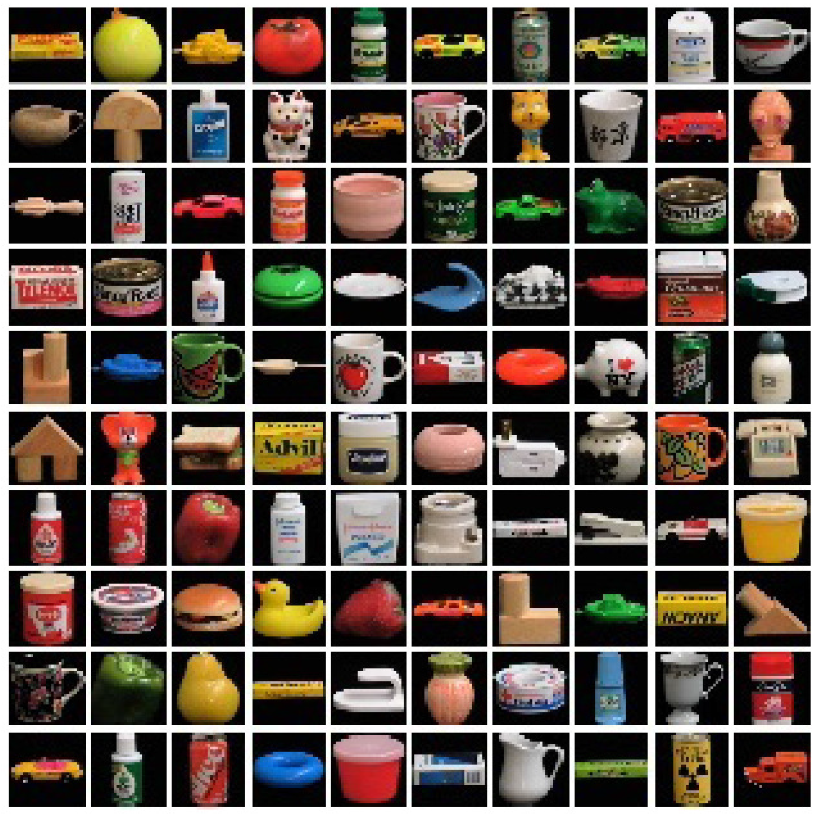
The second database used is the Columbia Object Image Library (COIL) database. The objects have a wide variety of complex geometric and reflectance characteristics. The COIL 20 database consists of 1440 gray-scale images of 20 objects. The objects were placed on a motorized turntable against a black background. Each object was placed in a stable configuration at approximately the centre of the table. Then, the turntable was rotated through 360 degrees to vary object pose with respect to a fixed camera. Images of the objects were taken at pose intervals of 5 degrees; this corresponds to 72 images per object. The images were also normalized, such that the larger of the two object dimensions (height and width) fits the image size of 128 × 128 pixels. When resizing, the aspect ratio was preserved. In addition to size normalization, every image was histogram stretched, i.e., the intensity of the brightest pixel was made 255, and the intensities of the other pixels were scaled accordingly. Consequently, the apparent scale of the object may change between different views of the object image, especially for the objects that are not symmetric with respect to the turntable axis. The (COIL-20) dataset is available online via ftp. It is a subset of the COIL-100 dataset of colour images of 100 objects (Figure 1), that is 7200 poses in total (COIL is available at http://www.cs.columbia.edu/CAVE/databases/).
Figure 1.
The Columbia Object Image Library (COIL-100).

We use a smaller set of 18 equally-spaced views per object in our experiments.
5.2. Experimenting with Real-World Data
In this section, we experiment with the curvature-based attributes extracted using the heat kernel embedding. We explore whether these attributes can be used for the purposes of graph-matching. The steps in implementing this process are as follows:
- We compute the adjacency matrices of the Delaunay triangulations of the detected feature points in each image.
- From the adjacency matrices, we construct the normalised Laplacian matrix for each graph in the database.
- For each graph, we then use the heat kernel embedding defined in Section 2.2 to embed the nodes of each graph as points residing on a manifold in a Euclidean space.
- The Euclidean distance between pairs of points in the Euclidean space is obtained from the heat kernel embedding at the values of and using the formula deduced in Section 2.4.
- From the embeddings, we compute two curvature-based representations for the graphs. The first is the sectional curvature associated with the edges, outlined in Section 3.1. The second is the Gaussian curvature on the triangles of the Delaunay triangulations extracted from the graphs, as outlined in Section 3.2.
- Both the sectional and Gaussian curvatures are used as graph features for the purposes of gauging the similarity of graphs. The similarities are computed using both the classical Hausdorff distance and the robust modified variant of the Hausdorff distance.
- Finally, we use the multidimensional scaling (MDS) procedure to embed the graphs into a low dimensional space where each graph is represented as a point in a 2D space.
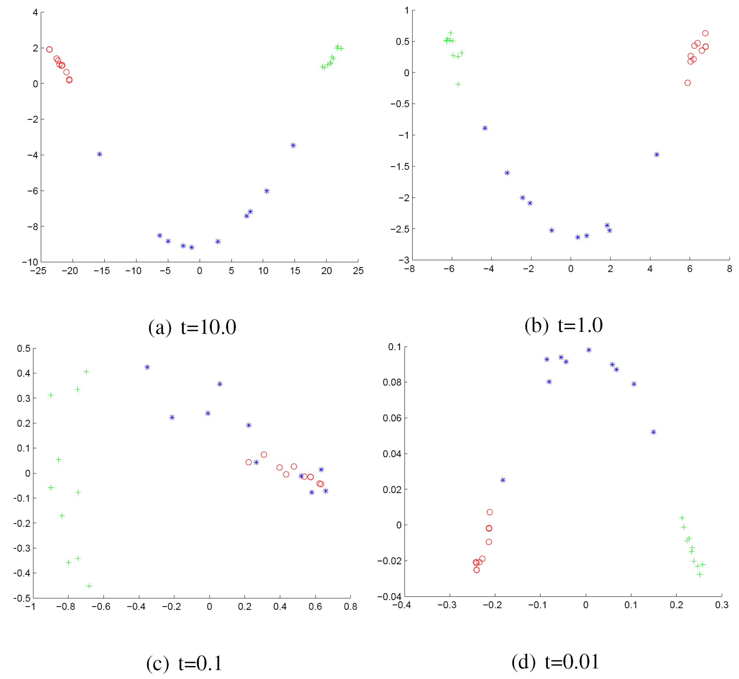
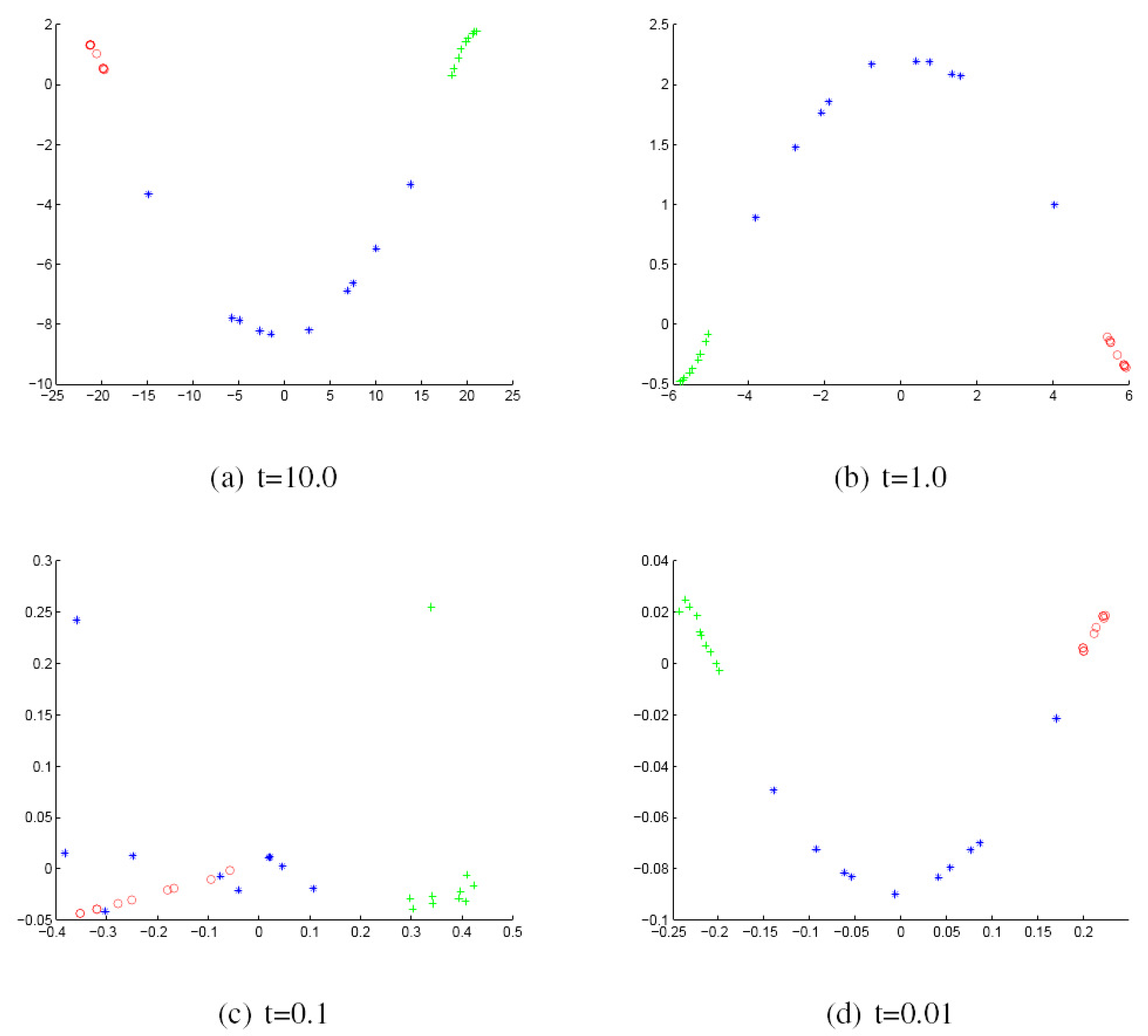
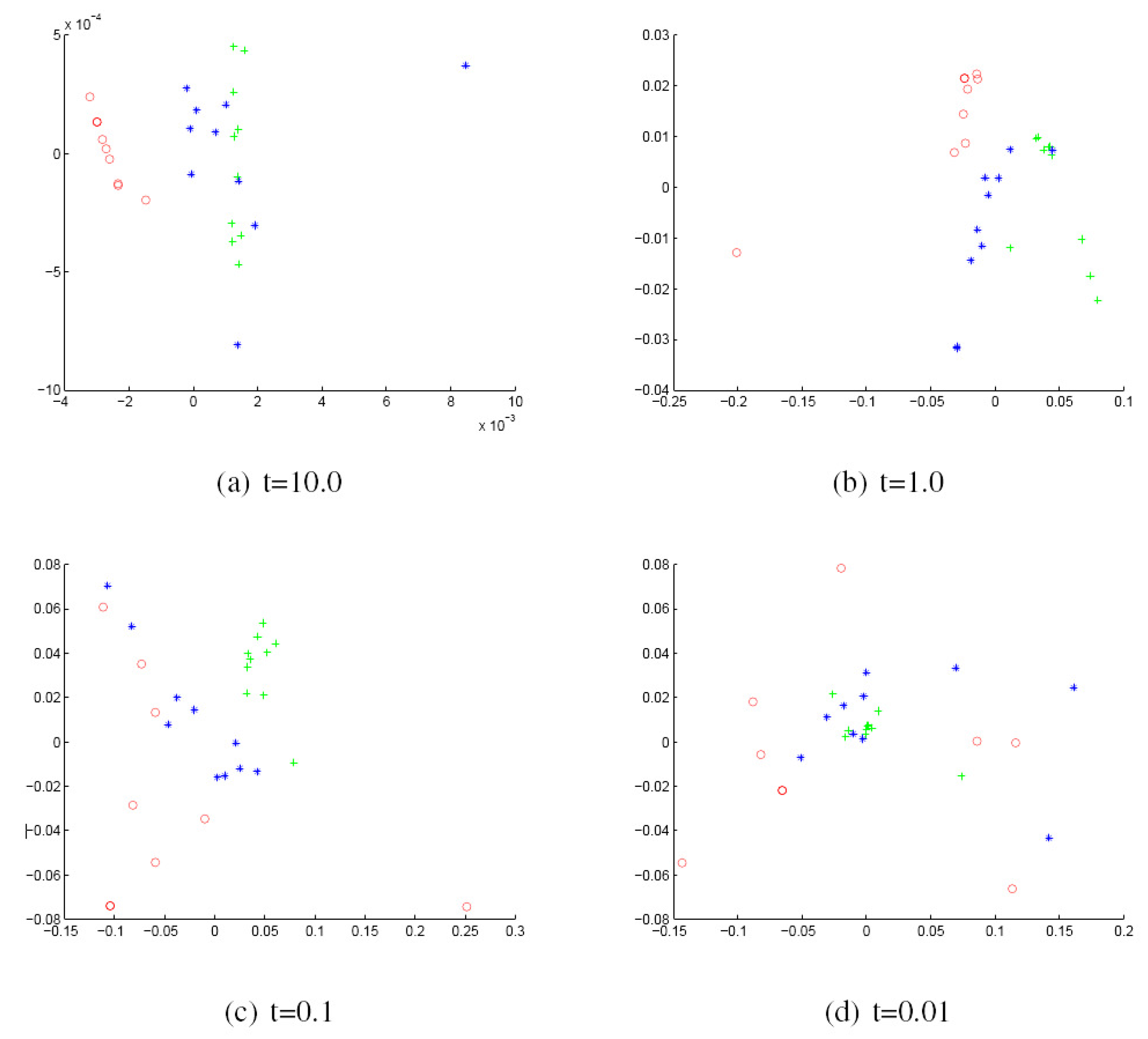
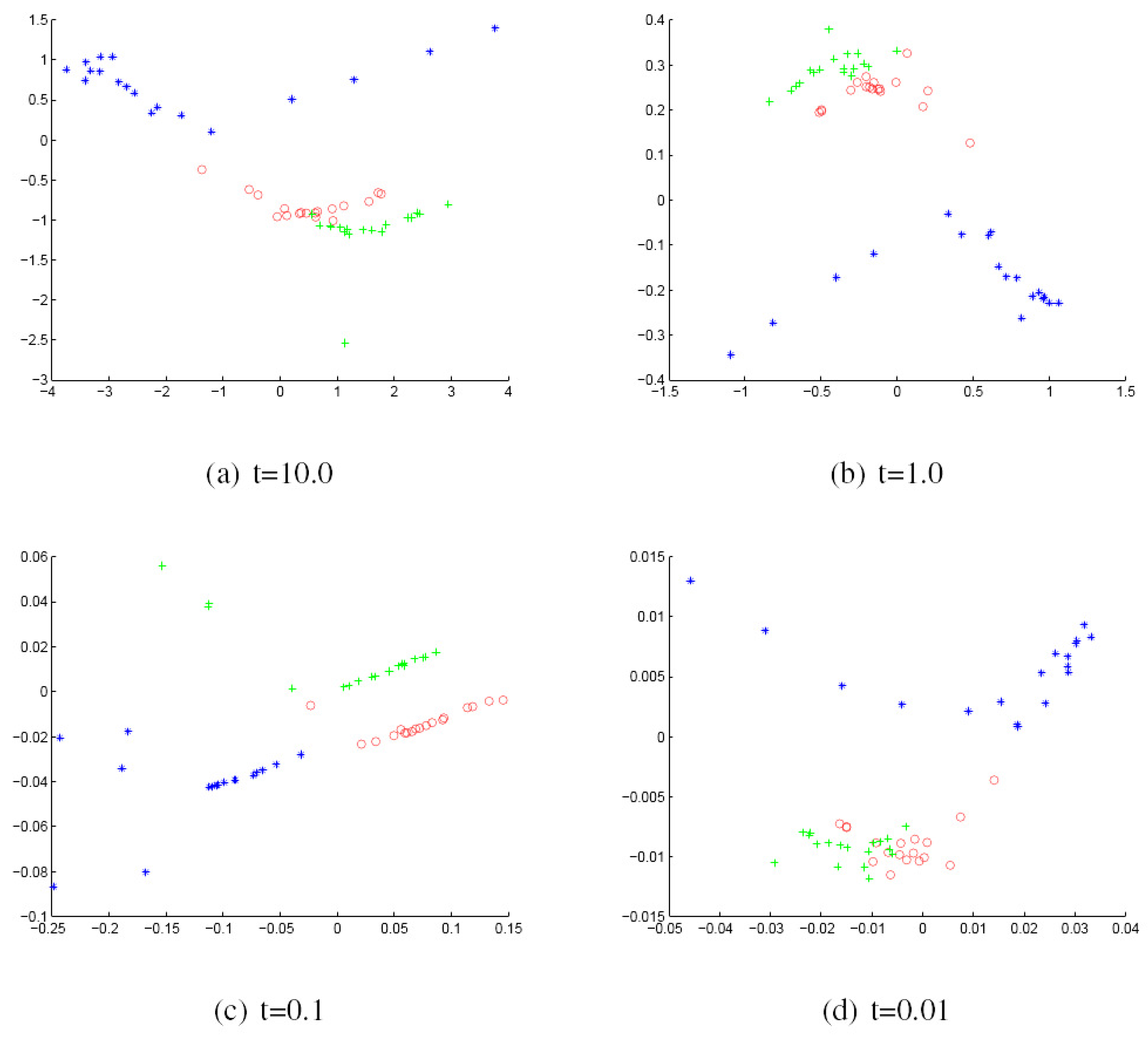
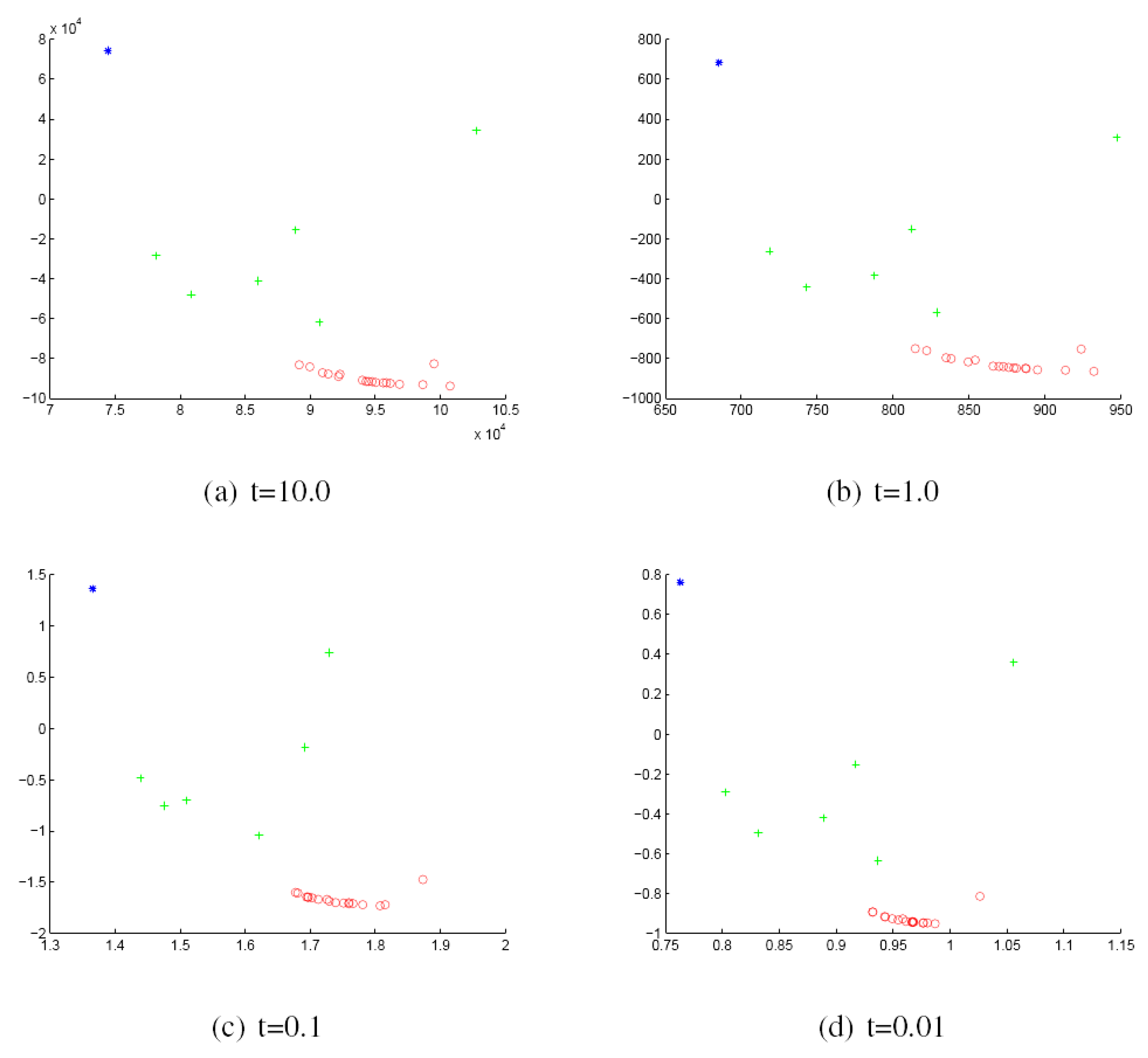
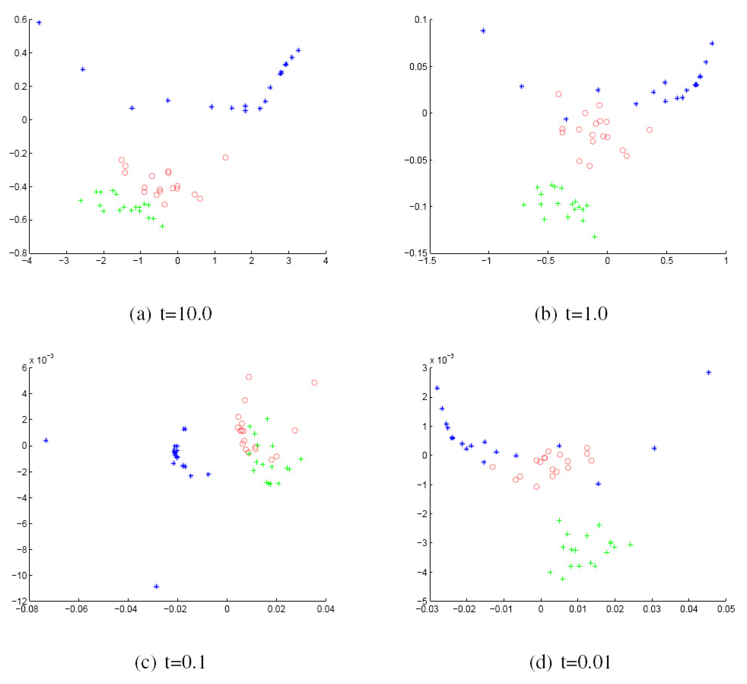
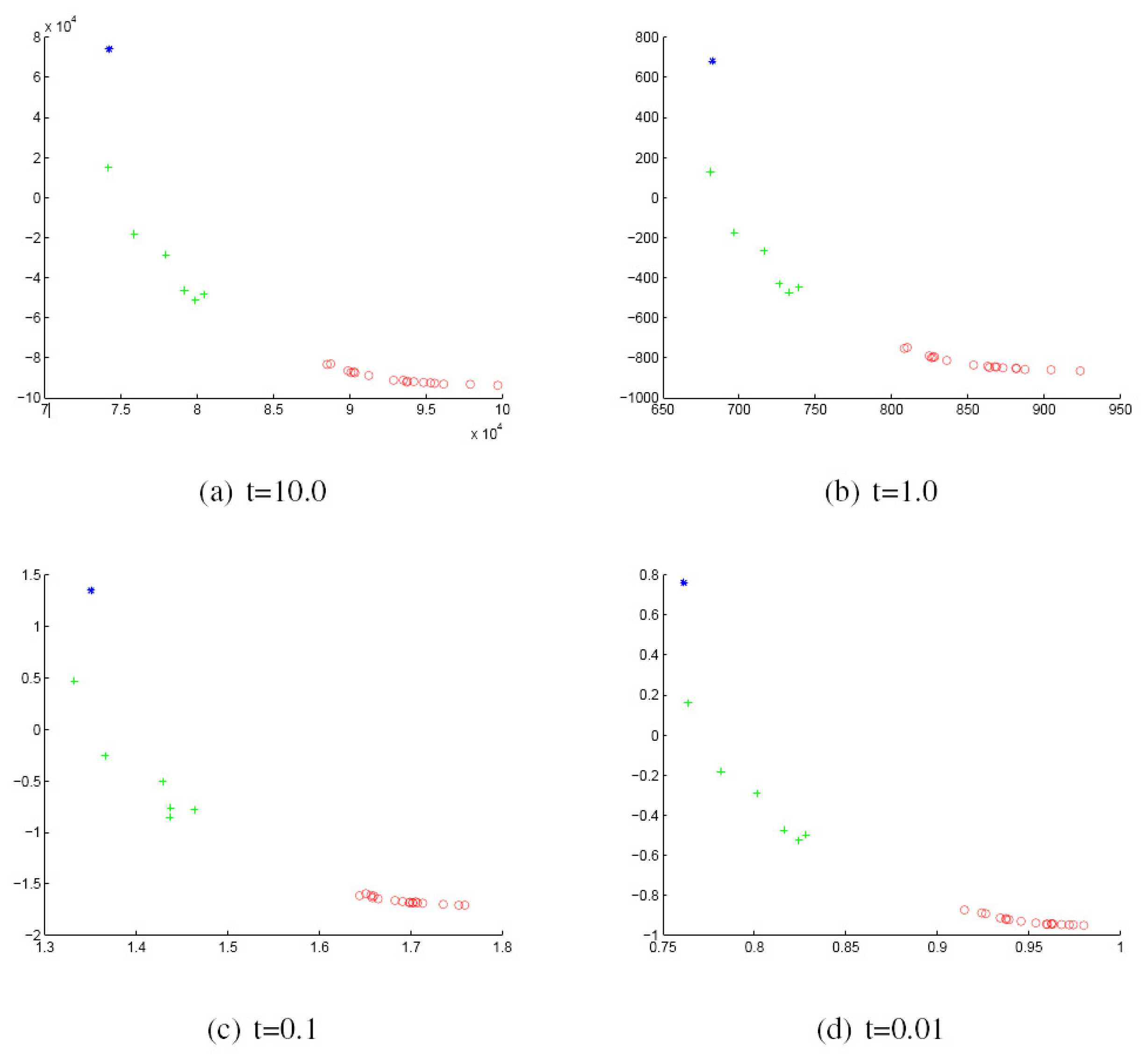
We commence by discussing the results obtained with the York Model Houses database. First, we show in Figure 2 and Figure 3 the results when using the Hausdorff distance (HD) to measure the (dis)similarity between pairs of graphs represented by the sectional and Gaussian curvatures, respectively. The sub-figures are ordered from left to right using the heat kernel embedding with the values t = 10.0, 1.0, 0.1 and 0.01, respectively. With the same order, Figure 4 and Figure 5 give the results obtained when using the modified Hausdorff distance (MHD).
Figure 2.
Multidimensional scaling (MDS) embedding obtained using Hausdorff distance (HD) for house data represented by the sectional curvatures residing on the edges. The x and y axes are the embedding coordinates corresponding to the leading two dimensions of the MDS embedding. The differently-coloured symbols denote different object classes.

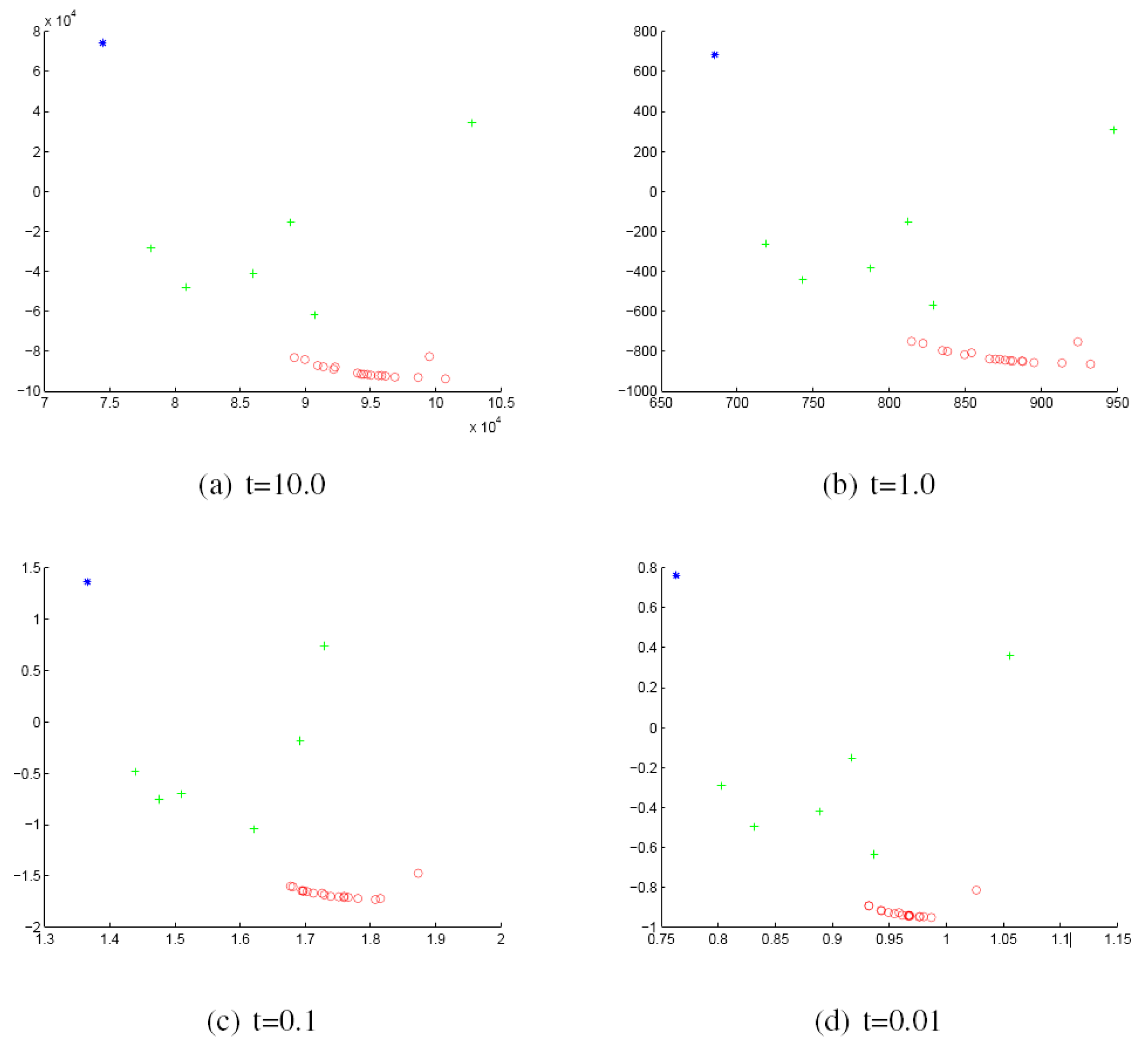
Figure 3.
MDS embedding obtained using HD for the houses data represented by the Gaussian curvature associated with the geodesic triangles. The x and y axes are the embedding coordinates corresponding to the leading two dimensions of the MDS embedding. The differently-coloured symbols denote different object classes.

Figure 4.
MDS embedding obtained using modified HD (MHD) for house data represented by the sectional curvatures residing on the edges.
Figure 4.
MDS embedding obtained using modified HD (MHD) for house data represented by the sectional curvatures residing on the edges.

Figure 5.
MDS embedding obtained using MHD for the houses data represented by the Gaussian curvature associated with the geodesic triangles. The x and y axes are the embedding coordinates corresponding to the leading two dimensions of the MDS embedding. The differently-coloured symbols denote different object classes.

To investigate the data in more detail, Table 1 shows the Rand index for the data as a function of t. This index is computed as follows:
- We commence by computing the mean for each cluster.
- Then, we compute the distance from each point to each mean.
- If the distance from the correct mean is smaller than those to remaining means, then the classification is correct; if not, then the classification is incorrect.
- The rand index is:= (♯ incorrect ) / ( ♯ incorrect + ♯ correct ).
We now discuss the results obtained when experimenting with the COIL database. Figure 6 and Figure 7 show the results when using the Hausdorff distance (HD) to measure the (dis)similarity between pairs of graphs represented by the Gaussian and sectional curvatures, respectively. The subfigures are ordered from left to right, top to bottom using the heat kernel embedding with the values and , respectively. With the same order, Figure 8 and Figure 9 give the results obtained when using the modified Hausdorff distance (MHD). Table 2 gives the Rand index for the data as a function of t.

| t = 10 | t = 1.0 | t = 0.1 | t = 0.01 | ||
|---|---|---|---|---|---|
| HD | Sectional curvature | 0.1000 | 0.1667 | 0.4333 | 0.0333 |
| HD | Gaussian curvature | 0.5000 | 0.1333 | 0.1000 | 0.5000 |
| MHD | Sectional curvature | 0.1333 | 0.2333 | 0.1333 | 0.0333 |
| MHD | Gaussian curvature | 0.1667 | 0.0333 | 0.1333 | 0.4000 |
Figure 6.
MDS embedding obtained using HD for Columbia Object Image Library (COIL) data represented by the sectional curvatures residing on the edges. The x and y axes are the embedding coordinates corresponding to the leading two dimensions of the MDS embedding. The differently-coloured symbols denote different object classes.

Figure 7.
MDS embedding obtained using HD for COIL data represented by the Gaussian curvatures associated with each node. The x and y axes are the embedding coordinates corresponding to the leading two dimensions of the MDS embedding. The differently-coloured symbols denote different object classes.

Figure 8.
MDS embedding obtained using MHD for COIL data represented by the sectional curvatures residing on the edges. The x and y axes are the embedding coordinates corresponding to the leading two dimensions of the MDS embedding. The differently-coloured symbols denote different object classes.
Figure 8.
MDS embedding obtained using MHD for COIL data represented by the sectional curvatures residing on the edges. The x and y axes are the embedding coordinates corresponding to the leading two dimensions of the MDS embedding. The differently-coloured symbols denote different object classes.

Figure 9.
MDS embedding obtained using MHD for COIL data represented by the Gaussian curvatures associated with each node. The x and y axes are the embedding coordinates corresponding to the leading two dimensions of the MDS embedding. The differently-coloured symbols denote different object classes.

| t = 10 | t = 1.0 | t = 0.1 | t = 0.01 | ||
|---|---|---|---|---|---|
| HD | Sectional curvature | 0.1667 | 0.2037 | 0.2407 | 0.2037 |
| HD | Gaussian curvature | 0.2222 | 0.0000 | 0.0000 | 0.2222 |
| MHD | Sectional curvature | 0.1852 | 0.1852 | 0.1667 | 0.2222 |
| MHD | Gaussian curvature | 0.2222 | 0.0926 | 0.0000 | 0.2222 |
The main features to note are as follows. For both the COIL and model house data, the structure of the MDS embeddings and the resulting Rand index depend strongly on the choice of the parameter t. In the embeddings, the data are clearly separated into distinct clusters, although the separability of the clusters depends strongly on the parameter t, but also on whether Hamming distance or modified Hamming distance is used. For both COIL and the model house data, the best classification results in terms of the Rand index are obtained with Gaussian curvature. Sectional curvature gives consistently rather poorer results. The effect of using Hamming distance versus modified Hamming distance is to change the structure of the embeddings. In the case of modified Hamming distance, the embeddings are “parabolic”, a feature associated with normalisation constraints applied to the distance measure. In this case, the normalisation comes from the constraint that probabilities sum to unity. Overall, this does not seem to affect the classification accuracy that can be achieved and is less significant than the difference resulting in the choice of sectional versus Gaussian curvature.
6. Conclusions
In this paper, we have investigated whether we can use the heat kernel to provide a geometric characterisation of graphs that can be used for the purposes of graph matching and clustering. This is a problem that can be addressed directly by using the spectral geometry of the combinatorial Laplacian. Performing a Young–Householder decomposition on the heat kernel maps the nodes of the graph to points in the manifold providing a matrix of embedding coordinates. Assuming that the manifold on which the nodes of the graph reside is locally Euclidean, the heat kernel is approximated by a Gaussian function of the geodesic distance between nodes. Then, the Euclidean distances between the nodes of the graph under study are estimated by equating the spectral and Gaussian forms of the heat kernel, and the geodesic distance (that is, the shortest distance on the manifold) is given by the floor of the path-length distribution, which can be computed from the Laplacian spectrum. With the embeddings in hand, we developed a graph characterisation based on differential geometry. To do so, we computed the sectional curvatures associated with the edges of the graph, making use of the fact that the sectional curvature can be determined by the difference between the geodesic and Euclidean distances between pairs of nodes. Taking this analysis one step further, we used the Gauss–Bonnet theorem to compute the Gaussian curvatures associated with triangular faces of the graph.
Characterising the graphs using sets of curvatures, defined either on the edges or the faces, we explored whether these characterizations can be used for the purpose of graph matching and clustering. To this end, we compute the similarities of the sets using robust variants of the Hausdorff distance, which allows us to compute the similarity of different graphs without knowing the correspondences between graph edges or faces.
Experimental results are provided for both sectional and Gaussian curvature characterizations of graphs. The two characterizations were used for gauging graph similarity. The graphs extracted from the York Houses and COIL-20 dataset show that the proposed characterizations proved to be effective for clustering graphs. However, the geometric attributes associated with the edges give a slightly better graph clustering.
Author Contributions
This work was done by Hewayda ElGhawalby under the direction and supervision of Edwin R. Hancock.
Conflicts of Interest
The authors declare no conflict of interest.
References
- Scholkopf, B.; Smola, A.; Muller, K.-R. Nonlinear component analysis as a kernel eigenvalue problem. Neural Comput. 1998, 10, 1299–1319. [Google Scholar] [CrossRef]
- Chung, F.R.K. Spectral Graph Theory; AMS: Ann Arbor, MI, USA, 1997; p. 92. [Google Scholar]
- De Verdi’ere, Y.C. Spectres De Graphes; Societe Mathematique de France: Paris, France, 1998. [Google Scholar]
- Linial, N.; London, E.; Rabinovich, Y. The geometry of graphs and some of its algorithmic applications. Combinatorica 1995, 15, 215–245. [Google Scholar] [CrossRef]
- Smola, A.; Kondor, R. Kernels and regularization on graphs. In Proceedings of the Conference on Learning Theory, Washington, DC, USA; 2003. [Google Scholar]
- Young, G.; Householder, A.S. Disscussion of a set of points in terms of their mutual distances. Psychometrika 1938, 3, 19–22. [Google Scholar] [CrossRef]
- Xiao, B.; Hancock, E.R. Heat kernel, Riemannian manifolds and Graph Embedding. LNCS 2004, 3138, 198–206. [Google Scholar]
- Atkins, J.E.; Boman, E.G.; Hendrickson, B. A Spectral Algorithm for Seriation and the Consecutive Ones Problem. SIAM J. Comput. 1998, 28, 297–310. [Google Scholar] [CrossRef]
- Shokoufandeh, A.; Dickinson, S.J.; Siddiqi, K.; Zucker, S.W. Indexing using a Spectral Encoding of Topological Structure. In Proceedings of the IEEE Computer Society Conference on Computer Vision and Pattern Recognition, Fort Collins, CO, USA, 23–25 June 1999; pp. 2491–2497.
- Shi, J.; Malik, J. Normalized cuts and image segmentation. IEEE Trans. Pattern Anal. Mach. Intell. 2000, 22, 888–905. [Google Scholar]
- Umeyama, S. An eigendecomposition approach to weighted graph matching problems. IEEE Trans. Pattern Anal. Mach. Intell. 1988, 10, 695–703. [Google Scholar] [CrossRef]
- Luo, B.; Hancock, E.R. Structural Graph Matching Using the EM Algorithm and Singular Value Decomposition. IEEE Trans. Pattern Anal. Mach. Intell. 2001, 23, 1120–1136. [Google Scholar]
- Yau, S.T.; Schoen, R.M. Lectures on Differential Geometry; Science Publication Co.: Somerville, MA, USA, 1988. [Google Scholar]
- Lebanon, G.; Lafferty, J.D. Hyperplane margin classifiers on the multinomial manifold. In Proceedings of the Twenty-First International Conference on Machine Learning, ICML’04, Banff, AB, Canada, 2004.
- Xiao, B.; Hancock, E.R. Trace Formula Analysis of Graphs. In Structural, Syntactic, and Statistical Pattern Recognition; Springer: Berlin, Germany, 2006; pp. 306–313. [Google Scholar]
- Spivak, M. A Comprehensive Introduction to Differential Geometry, 2nd ed.; Publish or Perish Inc.: Houston, TX, USA, 1979; Volume 1–5. [Google Scholar]
- Luxburg, U.V.; Belkin, M.; Bousquet, O. Consistency of Spectral Clustering; Technical Report 134; Max Planck Institute for Biological Cybernetics: Tubingen, Germany, 2004. [Google Scholar]
- Vaxman, A.; Ben-Chen, M.; Gotsman, C. A multi-resolution approach to heat kernels on discrete surfaces. ACM Trans. Graph. 2010, 29, 1–10. [Google Scholar] [CrossRef]
- Patane, G. wFEM heat kernel: Discretization and applications to shape analysis and retrieval. Comput. Aided Geom. Des. 2013, 30, 276–295. [Google Scholar] [CrossRef]
- Stillwell, J. Mathematics and Its History; Springer-Verlag: New York, NY, USA, 1974. [Google Scholar]
- Cox, T.; Cox, M. Multidimensional Scaling; Chapman-Hall: Boca Raton, FL, USA, 1994. [Google Scholar]
- Huttenlocher, D.; Klanderman, G.; Rucklidge, W. Comparing images using the Hausdorff distance. IEEE. Trans. Pattern Anal. Mach. Intell. 1993, 15, 850–863. [Google Scholar] [CrossRef]
- Dubuisson, M.; Jain, A. A modified Hausdorff distance for object matching. In Proceedings of the International Conference on Pattern Recognition (ICPR), Jerusalem, Israel, 9–13 October 1994; pp. 566–568.
- Luo, B.; Wilson, R.C.; Hancock, E.R. Spectral embedding of graphs. Pattern Recogint. 2003, 36, 2213–2230. [Google Scholar] [CrossRef]
- Luo, B.; Cross, A.; Hancock, E.R. Corner detection via topographic analysis of vector potential. Pattern Recognit. Lett. 1999, 20, 635–650. [Google Scholar] [CrossRef]
© 2015 by the authors; licensee MDPI, Basel, Switzerland. This article is an open access article distributed under the terms and conditions of the Creative Commons Attribution license (http://creativecommons.org/licenses/by/4.0/).
Share and Cite
MDPI and ACS Style
ElGhawalby, H.; Hancock, E.R. Heat Kernel Embeddings, Differential Geometry and Graph Structure. Axioms 2015, 4, 275-293. https://doi.org/10.3390/axioms4030275
AMA Style
ElGhawalby H, Hancock ER. Heat Kernel Embeddings, Differential Geometry and Graph Structure. Axioms. 2015; 4(3):275-293. https://doi.org/10.3390/axioms4030275
Chicago/Turabian StyleElGhawalby, Hewayda, and Edwin R. Hancock. 2015. "Heat Kernel Embeddings, Differential Geometry and Graph Structure" Axioms 4, no. 3: 275-293. https://doi.org/10.3390/axioms4030275