1. Introduction
The numerical solution of linear algebraic systems with symmetric positive definite (SPD) matrix is required in a broad range of applications, see e.g., [
1,
2,
3,
4,
5,
6]. We consider the case where the linear systems are large and investigate their iterative solution by preconditioned Krylov subspace methods [
4,
7,
8]. Our problem takes the form
where
is SPD. As a particular case of interest we also consider the case where
,
is a sparse full row-rank matrix and
is SPD. Systems of this kind arise in many contexts, such as the solution of linear and nonlinear least-squares problems and the solution of linear programming problems, see e.g., [
4,
6,
9]. The iterative solver employed is the Conjugate Gradient (CG) method or its variants [
4] and we propose its use in combination with limited memory preconditioners.
A preconditioner is denoted as limited memory if it can be stored compactly in a few vectors of length
m, and its product by a vector calls for scalar products and, possibly, sums of vectors [
10]. The limited memory preconditioners studied in this work belong to both the class of Incomplete Cholesky factorizations and to the class of Quasi-Newton preconditioners. Interestingly, they are approximate inverse preconditioners, i.e., they are approximations for
. We point out that the preconditioners proposed can also be used for solving symmetric saddle point linear systems iteratively. In fact, the application of constraint or augmented preconditioners involves the factorization of SPD matrices and a cheap approximation of such matrices or their inverses can be convenient [
11,
12].
Incomplete Cholesky factorizations use the entries of
H and may fail for a general SPD matrix, thus requiring strategies for recovering breakdowns. Further, memory requirements are difficult to predict if a drop tolerance is used to reduce the fill-in. For this reason, some factorizations allow a limited number of fill-ins to be created and the bound on the number of nonzero entries can be prefixed column-wise, typically taking into account the number of nonzero entries of the original matrix. Clearly, Incomplete Cholesky factorizations are not suitable when matrix
H is dense, which may be the case if
even though
A is sparse, see e.g., [
3]. A limited memory and breakdown-free “partial” Cholesky factorization was proposed in [
13,
14] and used in the solution of compressed sensing, linear and quadratic programming, Lasso problems, maximum cut problems [
3,
14,
15]. This preconditioner is built by computing a trapezoidal partial Cholesky factorization limited to a prefixed and small number of columns and by approximating the resulting Schur complement via its diagonal.
Limited memory Quasi-Newton preconditioners are a class of matrices built drawing inspiration from Quasi-Newton schemes for convex quadratic programming [
10]. Given a preconditioner (first-level preconditioner), Quasi-Newton preconditioners provide its update (second-level preconditioner) by exploiting a few vectors of dimension
m, i.e., information belonging to a low-dimensional subspace of
. Variants of the original Quasi-Newton scheme [
10] have been proposed in the literature. They differ in the choice of the low-dimensional subspace [
10,
16,
17,
18,
19] and several instances convey information from the iterative solver, possibly as approximate invariant subspaces.
In this paper, we analyze the connection between the partial Cholesky factorization [
13,
14] and a variant of the Quasi-Newton preconditioners. We show that the partial Cholesky factorization coincides with a Quasi-Newton preconditioner where the first-level preconditioner is diagonal and the low-dimensional subspace is constituted by a subset of columns of the identity matrix of dimension
m. This observation provides a way for building the partial Cholesky factorization which is alternative to the procedures in [
13,
14] and can offer some advantages in terms of computational effort. Due to the specific form of the low-dimensional subspace spanned by coordinate vectors in
, we denote the resulting preconditioner as the Coordinate Limited Memory Preconditioner (Coordinate-LMP). Successively, we propose a strategy for enriching the low-dimensional space that generates the partial Cholesky factorization, and thus enhancing the performance of the preconditioner; such a strategy is guided by the spectral analysis of
H preconditioned by the partial Cholesky factorization and it is analyzed from both the theoretical and practical point of view.
The paper is organized as follows. In
Section 2 we introduce the partial Cholesky factorization. In
Section 3 we show how the partial Cholesky factorization can be formulated as a Quasi-Newton type preconditioner and discuss the application of the two formulations in terms of computational effort. In
Section 4 we propose a strategy for enlarging the subspace in the Quasi-Newton formulation and analyze the spectral properties of the preconditioned matrix; the numerical performance of the resulting preconditioner are shown in
Section 5.
In the following, for any square matrix B, is the diagonal matrix with the same diagonal entries as B. For a SPD matrix , an eigenvalue is denoted either as or as , ; the minimum and maximum eigenvalues are denoted as and . The identity matrix of dimension q is denoted as . For indicating submatrices we borrow the Matlab notation. Preconditioned CG method is denoted as PCG.
2. A Limited Memory Partial Cholesky Preconditioner
The convergence behaviour of CG depends on the eigenvalue distribution of
H and the condition number of
H determines the worst-case behaviour of CG [
4,
8,
20,
21]. Further characterizations, possibly sharp, of the convergence behaviour can be gained from additional information on the eigenvalues. More specifically, it is known that if
A has
t distinct eigenvalues, then the CG method will converge in at most
t iterations, while CG applied to a matrix with
t tight eigenvalue clusters may not behave similarly as though it were applied to a matrix with
t distinct eigenvalues representing the individual clusters ([
21], [§5.6.5]).
A proposal for building a partial Cholesky factorization
P of
H was given by Gondzio in [
14] and Bellavia et al., in [
13]. It aims at clustering the largest eigenvalues of
H at one and reducing both the value of
with respect to
and the condition number of
with respect to
H. The first step is based on the observation that the trace
of
H is such that
and
since
H is symmetric and positive definite. Then, it is possible to handle the largest eigenvalues of
H by an heuristic technique where the largest
k,
, diagonal elements of
H are identified and the rank-
k partial Cholesky factorization of the corresponding columns of
H is performed. More specifically, suppose that
H can be partitioned as
where
and
contains the
k largest diagonal elements of
H (throughout the paper, the symmetric row and column permutations required to move the
k largest diagonal elements of
H to the
block are ignored to make the presentation simpler). To handle the large eigenvalues of
H, the Cholesky factorization limited to the first
k columns
is computed. We denote such factors as
, with
unit lower triangular,
, and
diagonal positive definite and observe that
H can be factorized as
being
S the Schur complement of
in
HFinally, the limited memory Partial Cholesky preconditioner P is obtained by approximating S with its diagonal and setting
The construction of the preconditioner
P is summarized in Algorithm 1 where we use the equalities
derived from Equation (
2).
| Algorithm 1 Limited Memory Partial Cholesky Preconditioner. |
Given the matrix-vector operators , . 1. Form the first k columns of H, i.e. . 2. Compute the diagonal entries of . 3. Compute as in Equations ( 5) and (6). Discard and . 4. Set . 5. Let P take the form Equation ( 4). |
This procedure is breakdown-free in exact arithmetic while Incomplete Cholesky factorizations employing a drop tolerance to reduce fill-in may fail for a general SPD matrix. The maximum storage requirement is known in advance and the upper bound on the number of nonzero entries in L is .
Forming the preconditioner calls for the complete diagonal of H. If H has the special form , its main diagonal can be constructed by performing m matrix-vector products , , and then computing . The products are cheap if A is sparse and involve no extra effort at all if A can be accessed row-wise and then retrieving the ith row comes at no extra cost. Moreover, the k products in Step 1 are expected to be cheaper than the products required by a CG-like method because the unit vectors are typically sparser than v.
The cost to perform the factorization Equation (
5) is negligible because matrix
has small dimension
k, while, using the first equation in Equation (6), the computation of
in Step 4 requires solving
triangular linear systems of dimension
k. Finally, in Step 4 computing
amounts to scaling the rows of
by the entries of
and performing
scalar products between vectors of dimension
k.
The spectral properties of
are analyzed in [
13] and reported below for completeness.
Theorem 1. Let k be a positive integer and P be as in Equation (4). Then, k eigenvalues of are equal to 1 and the remaining are equal to the eigenvalues of . Moreover, any eigenvalue lies in the interval . Proof of Theorem 1. Theorem 2.1 in [
13] proves that
k eigenvalues of
are equal to 1 and the remaining are equal to the eigenvalues of
. As for the bounds on the eigenvalues
, let
be an eigenvector of
. Then, by
we get
and
where we used the bounds
, see [
6]. ☐
We point out that the above preconditioner was used in [
13] in conjunction with Deflated-CG [
22] in order to handle also the smallest eigenvalues of
.
We conclude this section observing that the Partial Cholesky preconditioner can be formulated as an Approximate Inverse preconditioner. In fact, from (
4) matrix
can be factorized as the product of sparse matrices and takes the form
3. Limited Memory Quasi-Newton Type Preconditioners
Limited memory Quasi-Newton type preconditioners for SPD matrices were proposed in several works, see e.g., [
10,
17,
18,
19]. These preconditioners are generated using a small number
k of linear independent vectors in
.
Let us consider the formulation by Gratton et al. in [
19]. Suppose that a first preconditioner
M (called first-level preconditioner) is available. To improve the efficiency of the first-level preconditioner, a class of limited memory preconditioners (called second-level preconditioners) is defined on the base of the explicit knowledge of an
m by
k,
, full rank matrix Z. The aim of the second-level preconditioner is to capture directions lying in the range of
which have been left out by the first-level preconditioner and are slowing down the convergence of the CG solver; e.g., this is the case when the first-level preconditioner is able to cluster many eigenvalues at 1 with relatively few outliers.
Let be symmetric and positive definite, , , be a full column-rank matrix. The symmetric second-level preconditioner, say , takes the form
The spectral properties of
established in ([
19], [Lemma 3.3, Theorem 3.4]) are summarized below.
Theorem 2. Let H and M be symmetric and positive definite matrices of order m, , be a full column-rank matrix and Π be given by Equation (10). Then the matrix Π is positive definite. Let the positive eigenvalues of be sorted in nondecreasing order. Then the set of eigenvalues of can be split in two subsets:and Equation (
10) provides a general formulation for designing second-level preconditioners and was inspired by the BFGS inverse Hessian approximation in Quasi-Newton algorithms [
9]. In fact, if the BFGS method with exact linesearch is applied to a quadratic function, then the inverse Hessian approximation generated has the form of
in Equation (
10); we refer to ([
19], [§2]) for details on this interpretation. In the general setting, any set of linearly independent vectors can provide candidates for the columns of
Z and gives rise to a preconditioner of form Equation (
10);
k eigenvalues of
equal to 1 are obtained while the remaining eigenvalues satisfy the relevant interlacing property Equation (
11). On the other hand, specific choices for
Z guided by information on the problem at hand are preferable.
The preconditioner
has been specialized to the case of:
spectral-LMP where the columns of
Z consist of eigenvectors of
,
Ritz-LMP where the columns of
Z consist of Ritz vectors generated by the iterative linear solver,
Quasi-Newton-LMP where the columns of
Z consist of descent directions from optimization methods applied to continuous optimization problems, see e.g., [
10,
16,
17,
18,
19]. All these vectors are often available when systems with multiple right-hand sides of slowly varying sequence of systems are considered.
In this work, we propose and analyze preconditioners of the form Equation (
10) where the first-level preconditioner is the diagonal matrix
given in Equation (
4) and
Z is chosen as a suitable submatrix of the identity matrix
, i.e.,
consists of
k properly chosen columns of
H. Due to the fact that
Z consists of coordinate vectors in
we denote the resulting limited memory preconditioner as Coordinate-LMP. We start analyzing the case where
Forming the preconditioner
with Equation (
12) requires the steps listed in Algorithm 2.
| Algorithm 2 Coordinate Limited Memory Preconditioner. |
Given the matrix-vector operators , . 1. Form the first k columns of H, i.e. . 2. Compute the diagonal entries of . 3. Compute as in Equation ( 5). 4. Set , as in Equation ( 4). 5. Set M and Z as in Equation ( 12). 6. Let take the form Equation ( 10). |
In this specific variant, coincides with the inverse of the Partial Cholesky preconditioner P. We show this fact in the following theorem.
Theorem 3. Let k be a positive integer and P be as in Equation (4). If matrix Π has the form Equation (10) with M and Z as in Equation (12), then . Moreover, Proof of Theorem 3. By Equation (
9) it follows
Using Equations (
5) and (6) we obtain
and we conclude
Now consider
and first observe that the matrices appearing in Equation (
10) have the form:
Then,
i.e.,
. Finally, it is trivial to verify that
takes the upper block triangular form Equation (
13) which also provides the spectrum of
stated in Theorem 1. ☐
3.1. Application of the Preconditioners
In the previous section, we have shown that
and
can reduce to the same preconditioner. Clearly, their application as a preconditioner calls for matrix-vector products and this computational cost may depend on the formulation used i.e., either Equation (
9) or Equations (
10) and (
12). Let us analyze the cost for performing matrix-vector products of both
and
times a vector. As stated in
Section 2, the symmetric row and column permutations required to move the
k largest diagonal elements of
H to the
block are ignored to make the presentation simpler.
If the triangular factors in Equation (
9) have been formed, the application of the Partial Cholesky preconditioner
to a vector amounts to: two products of
by a vector
, one matrix-vector product with
,
scalar products in
,
k scalar products in
. It is worthy pointing out that the partial Cholesky factorization may be dense. In fact, for sparse Cholesky factorizations, permutation matrices are normally chosen to enhance the sparsity of the triangular factor, see e.g., [
4], while here we choose the
k columns in advance from the largest diagonals of
H.
The application of the Coordinate limited memory preconditioner
to a vector also calls for matrix-vector and scalar products. The computation of a product, say
, can be implemented efficiently using Equations (
10) and (
14) and performing the following steps
These steps call for two products of by a vector in , one matrix-vector product with , m scalar products in , k scalar products in . The cost for the product of Z by a vector is negligible due to the form of Z.
The computational cost for applying both
and
to a vector is expected to be comparable if the scalar products performed have similar computational effort; this is the case when the density of the first
k columns of
is similar to the density of the first
k columns of
H. On the other hand, if the density of the first
k columns of
is considerably larger than the density of the first
k columns of
H, the application of
is less convenient than the application of
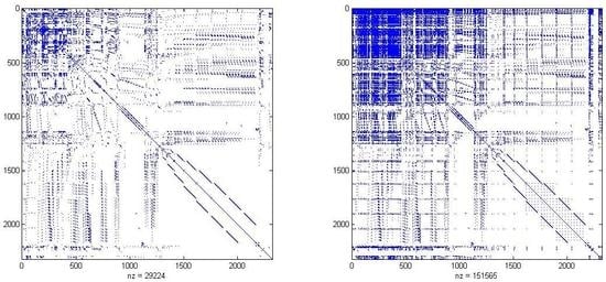
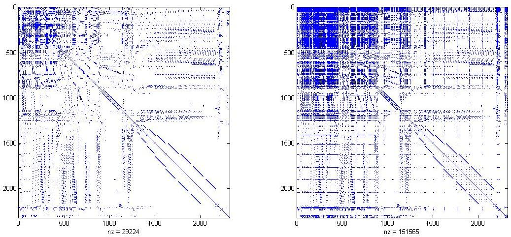
. This issue is shown in
Table 1 where we report on the numerical solution of four linear systems with matrices of the form
and matrix
A from the LPnetlib group in the University of Florida Sparse Matrix Collection [
23]. Preconditioned Conjugate Gradient [
4] is applied with both the Partial Cholesky preconditioner and the Coordinate-LMP , setting
. We display the dimension
of
A, the number of PCG iterations (Itns), the execution time in seconds (Time), the density of first
k columns of
(
), the density of the first
k columns of
H (
); the density is computed as the ratio between the number of nonzero entries and the overall number of entries of the mentioned submatrices.
We observe that is larger than in the first two tests and runs with are slower than with , while the two densities are similar in the last two runs as well as the timings obtained using and .
4. Enlarging the Subspace in the Coordinate-LMP Preconditioner
The Partial Cholesky preconditioner
P and the Coordinate-LMP
with first level preconditioner and subspace as in Equation (
12) aim at clustering the largest eigenvalues of
H. In this section we investigate how to enlarge the subspace
Z by means of information available from Algorithm 2 and the potential impact on the resulting preconditioner.
We consider the Coordinate-LMP Equation (
10), suppose to use again
as first level preconditioner, and to select a larger number of columns of
for the subspace defined by
Z. We let
with
ℓ being a positive integer, i.e., besides the first
k columns of
used in Equation (
12) we employ
ℓ more columns (for simplicity suppose the first
ℓ subsequent columns). The effect of this choice can be analyzed by considering the block partition of
H where the leading block
has dimension
q by
q, i.e.,
with
. Analogously, let us consider the block partition of
in Equation (
4) where the leading block
has dimension
q by
q, i.e.,
with
,
.
The spectral properties of the resulting Coordinate-LMP preconditioner are given in the following theorem.
Theorem 4. Let q be a positive integer, H and be symmetric positive definite matrices partitioned as in Equations (17) and (18). If matrix Π has the form Equation (10) with M and Z as in Equation (16), then has q eigenvalues equal to 1 and the remaining are equal to the eigenvalues of where Moreover any eigenvalue lies in the interval .
Proof of Theorem 4. Similarly to the proof of Theorem 3 we have
Then, by Equation (
10) we get
and consequently
Bounds on the eigenvalues
can be derived by fixing an eigenvector
of
. Then, by
we get
Thus, similarly to the proof of Theorem 1 it follows
since
and
[
6]. ☐
Remark 1. Let be the interval in the statement of Theorem 1 and be the interval in the statement of Theorem 4. It holds by the Cauchy Interlace Theorem [24] [p. 396]. Moreover, for any choice of trivially it holds Then, .
A comparison between bounds Equations (
7) and (8) and Equations (
22) and (23) suggests that the choice of the extremal diagonal elements of
S can be beneficial for improving, at a low computational cost, the clustering of the eigenvalues. In fact, choosing the extremal diagonal elements of
S promotes a reduction of the width of the interval containing the eigenvalues of
and this issue can favorably affect the performance of the iterative solver and the condition number of
.
Accordingly to Remark 1, let
and
be the intervals containing the eigenvalues of
with
generated by Equation (
12) and by Equation (
16) respectively. If the
ℓ largest diagonal entries of
are contained in matrix
in Equation (
18) and are separated from the remaining, then we obtain an increase of the lower bound of
with respect to lower bound of
; clearly, the better the
ℓ largest diagonal entries of
S are separated from the remaining elements of
the larger such increase is. Handling small eigenvalues of
seems to be convenient when enlarging the subspace
Z for
as the Partial Cholesky factorization is intended to take care of the largest eigenvalues of
H. Alternatively, if the
ℓ smallest diagonal entries of
S are contained in matrix
in Equation (
18) and are separated from the remaining, the upper bound of
is expected to be smaller than the upper bound of
.
As mentioned in
Section 2, in [
13] the partial Cholesky preconditioner was used in conjunction with Deflated-CG [
22] in order to handle the small eigenvalues of
. A rough approximation of the five smallest eigenvalues of
was injected into the Krylov subspace and yielded an improvement in some tests where Deflated-CG performed consistently fewer iterations than the usual CG. Although the deflation strategy brought undeniable benefits in terms of reducing the number of CG iterations, it involved an extra storage requirement and an extra cost which ultimately increased the overall solution time. In fact, the application of such a strategy was convenient when the eigenvalue information was used for a sequence of related linear systems, such as slowly varying systems or systems with multiple right-hand-side vectors. The strategy, presented in this section and based on selecting a prefixed number of the largest diagonal entries of
S, can be viewed as a cheap alternative procedure for handling the smallest eigenvalues of
.
5. Numerical Results
In this section we present a preliminary numerical validation of the performance of the Coordinate-LMP discussed in
Section 3 and
Section 4. All numerical experiments reported were performed on a Dell Latitude E4200 with a Intel(R) Cote(TM)2 Duo CPU U9600, @1.60 GHz, RAM 3.00 GB, using
Matlab and machine precision 2.2 × 10
−16.
We report results on a set of 18 linear systems where the coefficient matrix has the form
and the right-hand side is chosen as a normally distributed vector. In
Table 2 we list the name of matrices
used along with their dimensions and the density of both
A and
H computed as the ratio between the number of nonzero entries and the number of rows.
The first 15 matrices
A are taken from the groups LPnetlib and Meszaros in the University of Florida Sparse Matrix Collection [
23] and are constraint matrices of linear programming problems; in the associated linear systems we set
. The symbol “#” indicates when matrix
A was regularized by a shift
in order to get a numerically nonsingular matrix
H. We observe that both
A and
H are sparse and
H can be preconditioned by either Incomplete Cholesky factorizations or by our preconditioner. The last three systems were generated by the dual logarithmic barrier method [
3] applied to semidefinite programming relaxations of maximum cut problems. In these problems each row of
A is the unrolled representation of a rank-one
matrix and has one nonzero entry while
is a full matrix of dimension
defined as the Kronecker product of matrices of dimension
; consequently
H is full. Iterative methods are an option for solving these systems when
H cannot be allocated due to memory limitations [
3]. Incomplete Cholesky factorizations are not applicable while our preconditioner is viable.
The linear systems have been solved by Preconditioned Conjugate Gradient (PCG) method starting from the null initial guess and using the stopping criterion:
A failure is declared after 1000 iterations. The preconditioner
was applied as described in
Section 3.1.
The preconditioners used in our tests are: the Incomplete Cholesky factorization with zero-fill (IC(0)) computed by the built-in
Matlab function ichol, the Coordinate-LMP Equation (
12) with
, and the Coordinate-LMP Equation (
16) with
. Concerning the preconditioner with enlarged subspace Equation (
16), we consider the two strategies for enlarging
Z discussed at the end of
Section 4. The first strategy consists in selecting the columns of
associated to the
ℓ largest diagonal entries of
and in the following is denoted as
D2_large. The second strategy consists in selecting the columns of
associated to the
ℓ smallest diagonal entries of
and is denoted as
D2_small. In the following tables, the symbol “*” indicates a failure of CG solver while the symbol “†” indicates a failure in computing the Incomplete Cholesky factorization due to encountering a nonpositive pivot. The timing in seconds “Time” includes the construction of the preconditioner and the total execution time for PCG.
Our focus is on the reliability of the preconditioners tested and the computational gain provided. Regarding the latter issue, clearly it depends on both the number of PCG iterations and the cost of PCG per iteration.
Table 3 displays the results obtained solving the linear systems with: unpreconditioned CG, CG coupled with IC(0), CG coupled with the Coordinate-LMP Equation (
12), CG coupled with the Coordinate-LMP Equation (
16) and implemented using the
D2_large strategy. We report the number of PCG iterations (Itns) and the timing (Time). We observe that IC(0) factorization cannot be applied to the linear systems deriving from maximum cut problems since the resulting matrices
H are full, see
Table 2.
We start observing that CG preconditioned by the Coordinate-LMP preconditioners Equation (
16) and the
D2_large strategy solved all the systems, whereas a breakdown of IC(0) occurred five times out of fifteen as a nonpositive pivot was encountered. In eight systems out of ten, PCG with IC(0) required several iterations considerably smaller than the number of iterations performed with the limited memory preconditioners; correspondingly the execution time was favorable to IC(0) preconditioner. On the other hand, IC(0) preconditioner was less effective than the limited memory preconditioner on problems lp_osa_30 and lp_osa_60; this occurrence is motivated by several linear iterations comparable to that of limited preconditioners and the density of the Cholesky factor, cf.
Table 2. Finally, we point out that breakdowns of IC(0) can be recovered using Incomplete Cholesky factorization with very small threshold dropping and, consequently, high fill-in in the Incomplete Cholesky factor and computational overhead.
Comparing the limited memory preconditioners in terms of CG iterations, we observe that enlarging the subspace provides a reduction in such a number. The gain in CG iterations using the enlarged subspace is very limited for Problems lp_ganges, lp_dfl001 and lp_pds_10, while it varies between 3% and 52% for the remaining problems. Savings in time depend on both the reduction in the number of CG iterations performed and the cost of matrix-vector products. Namely, when the application of H is cheap, savings in PCG iterations between 11% and 31% do not yield a significant gain in time, see lp_degen3, lp_ken_13, lp_pilot; on the other hand when matrix-vector products are expensive, saving in time can occur even in the presence of a mild reduction in the number of CG iterations, see lp_pds_10, M2_K4_5000_maxcut, M3_K4_5000_maxcut. Interestingly the cost for forming and applying the preconditioners does not offset the convergence gain in PCG; this feature is evident from the value Time in runs where the reduction in PCG iterations is small, see lp_ganges and M5_3000_maxcut. In fact, we can expect that for matrices having the same eigenvalue distribution as our test matrices, and a substantial number of nonzero elements, significant reductions in computing time can be achieved with the Quasi-Newton preconditioner and enlarged subspace.
The effect of enlarging the subspace in the Coordinate-LMP preconditioner is further analyzed in
Table 4 where we report the minimum
and maximum
eigenvalues of the original matrix
H and of the preconditioned matrices
in four problems. We observe that the maximum eigenvalue of the preconditioned matrix is consistently smaller than the eigenvalue of
H and this shows the effectiveness of handling the largest eigenvalues by using the trace of
H. On the other hand, the smallest eigenvalue of the matrix preconditioned by the Partial Cholesky factorization (
with
) is moved towards the origin. As shown in the table, an increase in the value of the smallest eigenvalue can be obtained with the
D2_large implementation for
while the effect on the largest eigenvalue is marginal, as expected.
We conclude our presentation reporting the performance of the
D2_small implementation in
Table 5; the number of PCG iterations is displayed and part of the results in
Table 3 are repeated for clarity. We recall that the number of unit eigenvalues is
for both the
D2_large and
D2_small implementations, but the former strategy is more effective than the latter. In fact, the behaviour of the Partial Cholesky factorization and of the
D2_small implementation of the Coordinate-LMP preconditioner are similar in terms of PCG iterations, apart for problems lp_ganges, lp_sierra, cq9 where the latter approach is convenient. This confirms that the largest eigenvalues are handled by the Partial Cholesky factorization and a further reduction of the upper bound on the eigenvalues is not useful.
Summarizing, the results presented in this section seem to indicate that: enlarging the subspace with columns associated to the largest diagonal entries of the Schur complement
S in Equation (
3) reduces the number of PCG iterations; the cost for forming and applying the preconditioner with enlarged subspace does not offset the gain from reducing PCG iterations; saving in times are obtained accordingly to the cost of matrix-vector products in PCG. Moreover, the Quasi-Newton preconditioner proposed is suitable for application to dense matrices
H of the form
,
A sparse, where computing the Incomplete Cholesky factor is too expensive in terms of computational cost and/or storage requirement.


