Neutrosophic Incidence Graphs With Application

Abstract

In this research study, we introduce the notion of single-valued neutrosophic incidence graphs. We describe certain concepts, including bridges, cut vertex and blocks in single-valued neutrosophic incidence graphs. We present some properties of single-valued neutrosophic incidence graphs. We discuss the edge-connectivity, vertex-connectivity and pair-connectivity in neutrosophic incidence graphs. We also deal with a mathematical model of the situation of illegal migration from Pakistan to Europe.

1. Introduction

The concept of graph theory was introduced by Euler. A crisp graph shows the relations between the elements of the vertex set. A weighted graph gives the extent of these relations. Many problems can be solved if proper weights are given. However, in many situations, the weights may not known, and the relationship is uncertain. Hence, a fuzzy relation can be used to handle such situations. Rosenfeld [1] developed the concept of a fuzzy graph. He also discussed several concepts like edges, paths, bridges and connectedness in a fuzzy graph. Most of the theoretical development of fuzzy graph theory is based on Rosenfeld’s initial work. Bhutani et al. [2,3] introduced the advance concepts in fuzzy graphs.

Sometimes when the relationship between the elements of the vertex set is indeterminate, the fuzzy graph and its extension fails. This indeterminacy can be overcome by using single-valued neutrosophic graphs [4].

Dinesh, in [5], introduced the concept of unordered pairs of vertices which are not incident with end vertices. The fuzzy incidence graph not just shows the relations between vertices, but also provides information about the influence of a vertex on an edge. Dinesh extended the idea of the fuzzy incidence graph in [6] by introducing new concepts in this regard. Later, Methew et al. [7] discussed the connectivity concepts in fuzzy incidence graphs. Malik et al. [8] applied the notion of the fuzzy incidence graph in problems involving human trafficking. They discussed the role played by the vulnerability of countries and their government’s response to human trafficking. Methew et al. [9] studied fuzzy incidence blocks and their applications in illegal migration problems. They used fuzzy incidence graphs as a model for a nondeterministic network with supporting links. They used fuzzy incidence blocks to avoid the vulnerable links in the network.

The paper is organized as follows: In Section 1, we give some preliminary notions and terminologies of fuzzy incidence graphs which are needed to understand the extended concept of the single-valued neutrosophic incidence graph. In Section 2, we present the definition of a single-valued neutrosophic incidence graph. We also discuss the edge-connectivity, vertex-connectivity and pair-connectivity in neutrosophic incidence graphs. 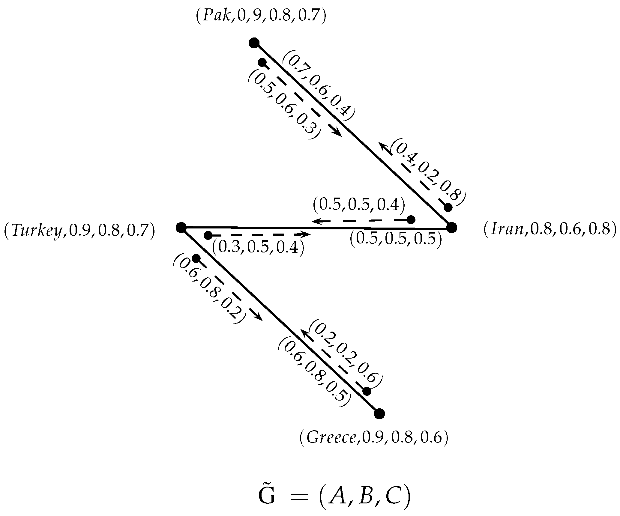In Section 3, we give a mathematical model of the situation of illegal migration from Pakistan to Europe. Finally, the paper is concluded by some remarks in Section 4. Below we present some preliminary definitions from [6] and [4]. For further study on these topics, the readers are referred to references [1,7,8,9,10,11,12,13,14,15,16].

Let $G=(V,E)$ be a graph on a nonempty set, V. Then, $G^{\prime }=(V,E,I)$ is called an incidence graph, where $I\subseteq V\times E$. The elements of I are called incidence pairs or simply, pairs.

A fuzzy incidence graph of an incidence graph, $G^{\prime }=(V,E,I)$, is an ordered-triplet, $\tilde{G}$ = $(\mu ,\lambda ,\psi )$, where $\mu$ is a fuzzy subset of V, $\lambda$ is a fuzzy relation of V, and $\psi$ is a fuzzy subset of I such that

$$\psi (x,xy)\le min\left\{\mu \right(x),\lambda (xy\left)\right\},\forall x\in V,xy\in E.$$

We may compare elements of two neutrosophic sets A and B, that is

$$(T_A\left(x\right),I_A\left(x\right),F_A\left(x\right))<(T_B\left(x\right),I_B\left(x\right),F_B\left(x\right))$$

$$\Rightarrow T_A\left(x\right)<T_B\left(x\right),I_A\left(x\right)<I_B\left(x\right),F_A\left(x\right)>F_B\left(x\right).$$

2. Single-Valued Neutrosophic Incidence Graphs

Definition 1.

A single-valued neutrosophic incidence graph of an incidence graph, $G^{\prime }=(V,E,I)$, is an ordered-triplet, $\tilde{G}=$ $(A,B,C)$, such that

1. 

A is a single-valued neutrosophic set on V.

2. 

B is a single-valued neutrosophic relation on V.

3. 

C is a single-valued neutrosophic subset of $V\times E$ such that

$$\begin{array}{ccc}{T}_C(x,xy)\hfill & \hfill \le & min\{T_A\left(x\right),T_B\left(xy\right)\},\hfill \\ I_C(x,xy)\hfill & \hfill \le & min\{I_A\left(x\right),I_B\left(xy\right)\},\hfill \\ F_C(x,xy)\hfill & \hfill \le & max\{F_A\left(x\right),F_B\left(xy\right)\},\forall x\in V,xy\in E.\hfill \end{array}$$

Here, we discuss an example of a single-valued neutrosophic incidence graph (SVNIG).

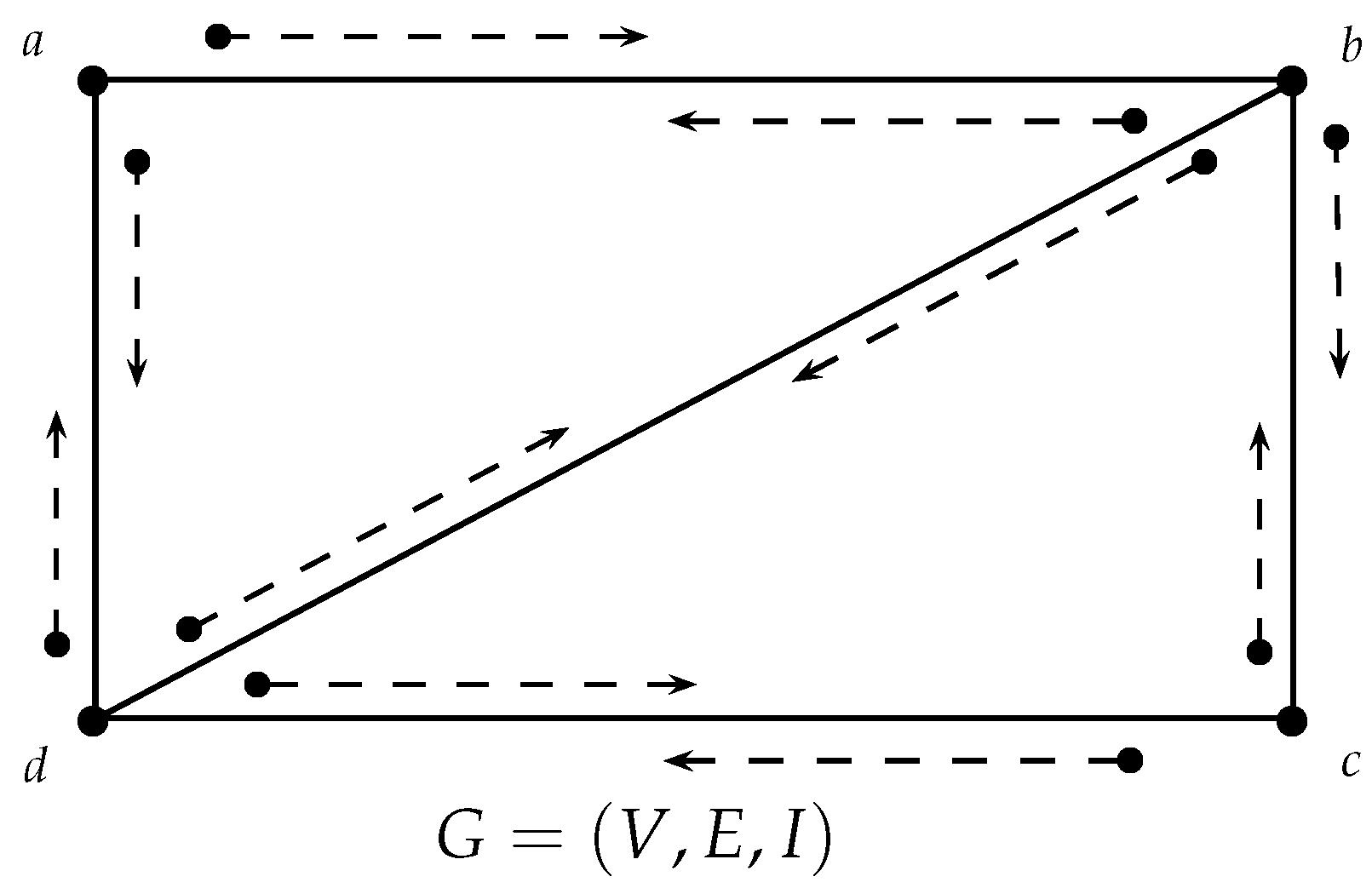
Example 1.

Consider an incidence graph, $G=(V,E,I)$, such that $V=\{a,b,c,d\}$, $E=\{ab,bc,bd,cd,ad\}$ and $I=\left\{\right(a,ab),(b,ab),(b,bc),(c,bc),(b,bd),(d,bd),(c,cd),(d,cd),(d,ad),(a,ad\left)\right\}$, as shown in Figure 1.

Let $\tilde{G}=$ $(A,B,C)$ be a single-valued neutrosophic incidence graph associated with G, as shown in Figure 2, where

$$\begin{array}{cc}\hfill A=& \left\{\right(a,0.2,0.5,0.8),(b,0.3,0.5,0.1),(c,0.9,0.9,0.1),(d,0.8,0.1,0.2\left)\right\},\hfill \\ \hfill B=& \left\{\right(ab,0.2,0.4,0.7),(bc,0.3,0.4,0.1),(bd,0.1,0.1,0.1),(cd,0.7,0.1,0.2),(ad,0.1,0.1,0.5\left)\right\},\hfill \\ \hfill C=& \left\{\right((a,ab),0.2,0.3,0.7),((b,ab),0.1,0.4,0.6),((b,bc),0.3,0.3,0.1),((c,bc),0.2,0.3,0.1),\hfill \\ & \left(\right(b,bd),0.1,0.1,0.1),\left(\right(d,bd),0.1,0.1,0.2),\left(\right(c,cd),0.7,0.1,0.2),\left(\right(d,cd),0.7,0.1,0.2)\hfill \\ & \left(\right(d,ad),0.1,0.1,0.4),\left(\right(a,ad),0.1,0.1,0.5)\}.\hfill \end{array}$$

Definition 2.

The support of an SVNIG $\tilde{G}=$ $(A,B,C)$ is denoted by $G^{*}=(A^{*},B^{*},C^{*})$ where

$$\begin{array}{cccc}\hfill A^{*}& =\hfill & \hfill \mathit{support}\mathit{of}A& =\{x\in V:T_A\left(x\right)>0,I_A\left(x\right)>0,F_A\left(x\right)>0\},\hfill \\ \hfill B^{*}& =\hfill & \hfill \mathit{support}\mathit{of}B& =\{xy\in E:T_B\left(xy\right)>0,I_B\left(xy\right)>0,F_B\left(xy\right)>0\},\hfill \\ \hfill C^{*}& =\hfill & \hfill \mathit{support}\mathit{of}C& =\{(x,xy)\in I:T_C(x,xy)>0,I_C(x,xy)>0,F_C(x,xy)>0\}.\hfill \end{array}$$

Now we introduce the concepts of edge, pair, walk, trail, path and connectedness in an SVNIG.

Definition 3.

If $xy$ ∈ $B^{*}$, then $xy$ is an edge of the SVNIG $\tilde{G}=$ $(A,B,C)$ and if $(x,xy),(y,xy)\in C^{*}$, then $(x,xy)$ and $(y,xy)$ are called pairs of $\tilde{G}$.

Definition 4.

A sequence

$$\begin{array}{cc}\hfill P:& u_0,(u_0,u_0{u}_1),u_0{u}_1,(u_1,u_0{u}_1),u_1,(u_1,u_1{u}_2),u_1{u}_2,(u_2,u_1{u}_2),u_2,\dots ,\hfill \\ & u_{n-1},(u_{n-1},u_{n-1}{u}_n),u_{n-1}{u}_n,(u_n,u_{n-1}{u}_n),u_n\hfill \end{array}$$

of vertices, edges and pairs in $\tilde{G}$ is a walk. It is a closed walk if $u_0=u_n$.

In the above sequence, if all edges are distinct, then it is a trail, and if the pairs are distinct, then it is an incidence trail. P is called a path if the vertices are distinct. A path is called a cycle if the initial and end vertices of the path are same. Any two vertices of $\tilde{G}$ are said to be connected if they are joined by a path.

Example 2.

In the example presented earlier

$$P_1:a,(a,ab),ab,(b,ab),b,(b,bd),bd,(d,bd),d,(d,da),da,(a,da),a$$

is a walk. It is a closed walk since the initial and final vertices are same, i.e., it is not a path, but it is a trail and an incidence trail.

$$P_2:a,(a,ab),ab,(b,ab),b,(b,bd),bd,(d,bd),d$$

$P_2$ is a walk, path, trail and an incidence trail.

Definition 5.

Let $\tilde{G}=$ $(A,B,C)$ be a nSVNIG. Then, $\tilde{H}$ = $(L,M,N)$ is a single-valued neutrosophic incidence subgraph of $\tilde{G}$ if $L\subseteq A$, $M\subseteq B$ and $N\subseteq C$. $\tilde{H}$ is a single-valued neutrosophic incidence spanning subgraph of $\tilde{G}$ if $L^{*}=A^{*}$.

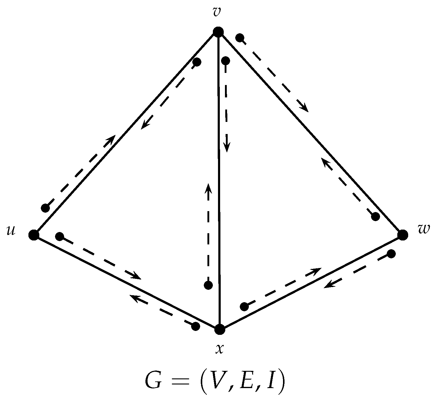
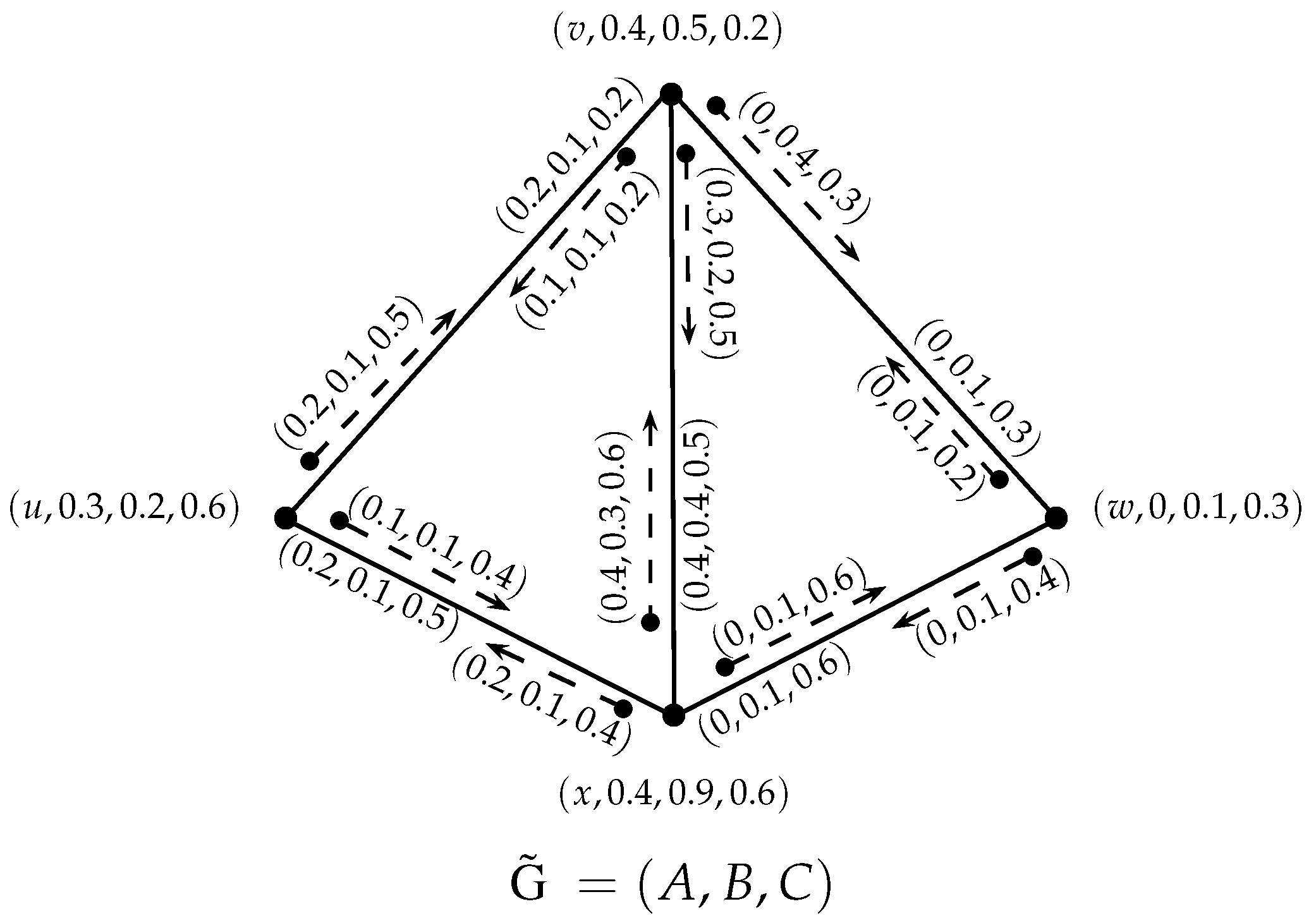
Definition 6.

In an SVNIG, the strength of a path, P, is an ordered triplet denoted by $S\left(P\right)=$ $(s_1,s_2,s_3)$, where

$$\begin{array}{cc}\hfill s_1& =min\{T_B\left(uv\right):uv\in P\},\hfill \\ \hfill s_2& =min\{I_B\left(uv\right):uv\in P\},\hfill \\ \hfill s_3& =max\{F_B\left(uv\right):uv\in P\}.\hfill \end{array}$$

Similarly, the incidence strength of a path, P, in an SVNIG is denoted by $IS\left(P\right)=(i{s}_1,i{s}_2,i{s}_3)$, where

$$\begin{array}{cc}\hfill i{s}_1& =min\{T_C(u,uv):(u,uv)\in P\},\hfill \\ \hfill i{s}_2& =min\{I_C(u,uv):(u,uv)\in P\},\hfill \\ \hfill i{s}_3& =max\{F_C(u,uv):(u,uv)\in P\}.\hfill \end{array}$$

Example 3.

Let $G=(V,E,I)$ be an incidence graph, as shown in Figure 3, and $\tilde{G}=$ $(A,B,C)$ is an SVNIG associated with G, which is shown in Figure 4.

Clearly, $P:u,(u,uv),uv,(v,uv),v,(v,vx),vx,(x,vx),x$ is a path in $\tilde{G}$.

The strength of the path, P, is $S\left(P\right)=(0.2,0.1,0.5)$, and the incidence strength of P is $IS\left(P\right)=(0.1,0.1,0.6)$.

Definition 7.

In an SVNIG, $\tilde{G}=$ $(A,B,C)$ the greatest strength of the path from l to m, where l,m $\in A^{*}\cup B^{*}$ is the maximum of strength of all paths from l to m.

$$\begin{array}{cc}\hfill S^{\infty }(l,m)=& max\{S\left(P_1\right),S\left(P_2\right),S\left(P_3\right),\dots \}\hfill \\ \hfill =& (s_1^{\infty },s_2^{\infty },s_3^{\infty })\hfill \\ \hfill =& \left(max(s_{11},s_{12},s_{13},\dots ),max\left(s_{21},s_{22},s_{23},\dots \right),min(s_{31},s_{32},s_{33},\dots )\right).\hfill \end{array}$$

$S^{\infty }$(l,m) is sometimes called the connectedness between l and m.

Similarly, the greatest incidence strength of the path from l to m, where l,m $\in A^{*}\cup B^{*}$ is the maximum incidence strength of all paths from l to m.

$$\begin{array}{cc}\hfill I{S}^{\infty }(l,m)=& max\{IS\left(P_1\right),IS\left(P_2\right),IS\left(P_3\right),\dots \}\hfill \\ \hfill =& (i{s}_1^{\infty },i{s}_2^{\infty },i{s}_3^{\infty })\hfill \\ \hfill =& \left(max(i{s}_{11},i{s}_{12},i{s}_{13},\dots ),max\left(i{s}_{21},i{s}_{22},i{s}_{23},\dots \right),min(i{s}_{31},i{s}_{32},i{s}_{33},\dots )\right),\hfill \end{array}$$

where $P_j$, $j=1,2,3,\dots$ are different paths from l to m.

$I{S}^{\infty }(l,m)$ is sometimes referred as the incidence connectedness between l and m.

Example 4.

In the SVNIG given in Figure 4, the total paths from vertex u to w are as follows:

$$\begin{array}{cc}\hfill P_1& :u,(u,ux),ux,(x,ux),x,(x,wx),wx,,(w,wx),w.\hfill \\ \hfill P_2& :u,(u,uv),uv,(v,uv),v,(v,vw),vw,(w,vw),w.\hfill \\ \hfill P_3& :u,(u,uv),uv,(v,uv),v,(v,vx),vx,(x,vx),x,(x,wx),wx,(w,wx),w.\hfill \\ \hfill P_4& :u,(u,ux),ux,(x,ux),x,(x,vx),vx,(v,vx),v,(v,vw),vw,(w,vw),w.\hfill \end{array}$$

The corresponding incidence strengths of each path are

$$\begin{array}{cc}\hfill IS\left(P_1\right)& =(s_{11},s_{21},s_{31})=(0,0.1,0.6),\hfill \\ \hfill IS\left(P_2\right)& =(s_{12},s_{22},s_{32})=(0,0.1,0.5),\hfill \\ \hfill IS\left(P_3\right)& =(s_{13},s_{23},s_{33})=(0,0.1,0.6),\hfill \\ \hfill IS\left(P_4\right)& =(s_{14},s_{24},s_{34})=(0,0.1,0.6).\hfill \end{array}$$

Now, the greatest incidence strength of the path from u to w is calculated as follows:

$$\begin{array}{cc}\hfill I{S}^{\infty }(u,w)& =max\{IS\left(P_1\right),IS\left(P_2\right),IS\left(P_3\right),IS\left(P_4\right)\}\hfill \\ & =(max\{i{s}_{11},i{s}_{12},i{s}_{13},i{s}_{14}\},max\{i{s}_{21},i{s}_{22},i{s}_{23},i{s}_{24}\},min\{i{s}_{31},i{s}_{32},i{s}_{33},i{s}_{34}\})\hfill \\ & =(max\{0,0,0,0\},max\{0.1,0.1,0.1,0.1\},min\{0.6,0.5,0.6,0.6\left\}\right)\hfill \\ & =(0,0.1,0.5).\hfill \end{array}$$

Definition 8.

An SVNIG, $\tilde{G}=$ $(A,B,C)$, is a cycle if, and only if, the underlying graph, $G^{*}=(A^{*},B^{*},C^{*})$, is a cycle.

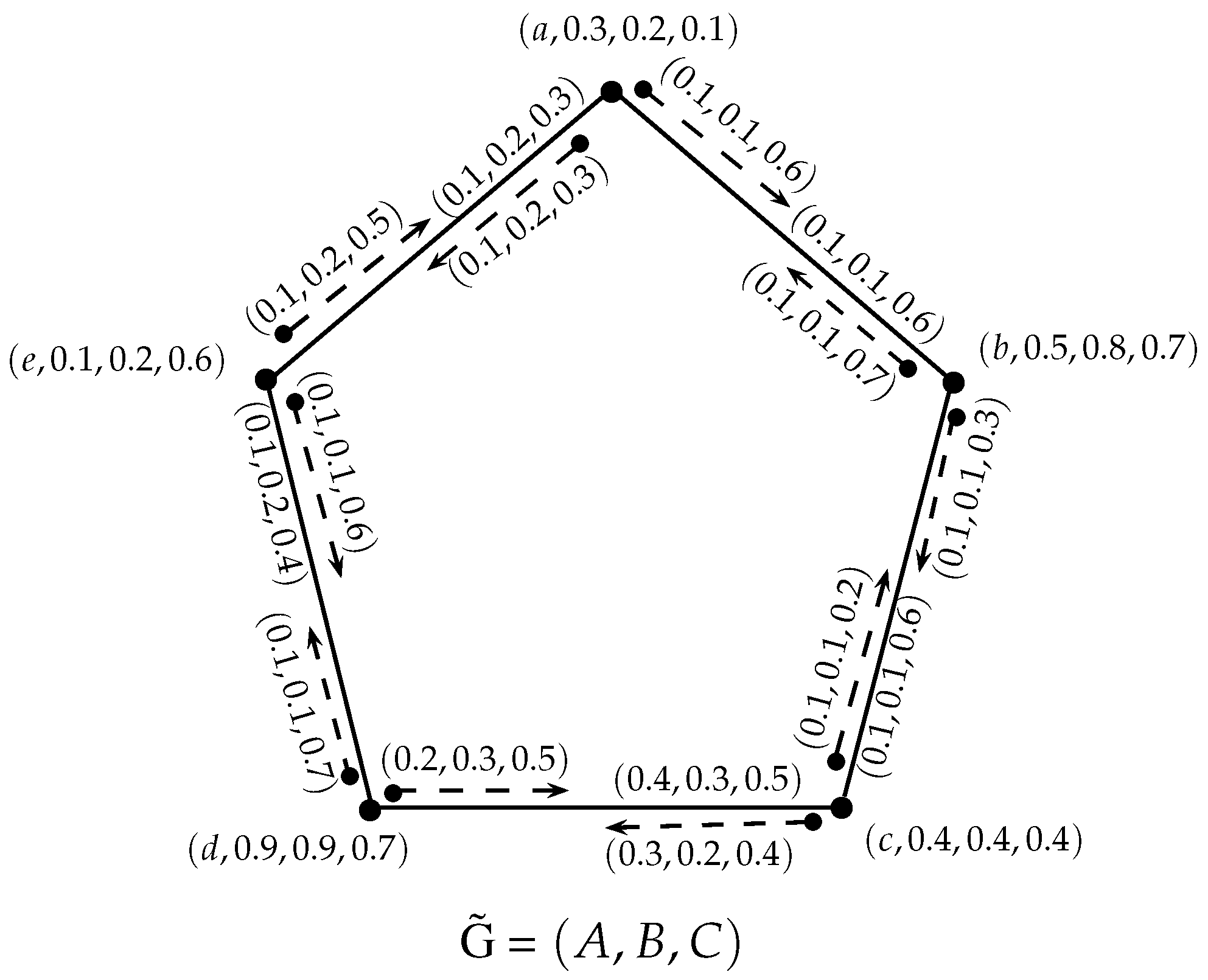
Definition 9.

The SVNIG $\tilde{G}=$ $(A,B,C)$ is a neutrosophic cycle if, and only if, $G^{*}=(A^{*},B^{*},C^{*})$ is a cycle and there exists no unique edge, $xy\in B^{*}$, such that

$$\begin{array}{ccc}\hfill T_B\left(xy\right)& =\hfill & \hfill min\{T_B\left(uv\right):uv\in B^{*}\},\\ \hfill I_B\left(xy\right)& =\hfill & \hfill min\{I_B\left(uv\right):uv\in B^{*}\},\\ \hfill F_B\left(xy\right)& =\hfill & \hfill max\{F_B\left(uv\right):uv\in B^{*}\}.\end{array}$$

Definition 10.

The SVNIG $\tilde{G}=$ $(A,B,C)$ is a neutrosophic incidence cycle if, and only if it is a neutrosophic cycle and there exists no unique pair, $(x,xy)\in C^{*}$, such that

$$\begin{array}{ccc}\hfill T_C(x,xy)& =\hfill & \hfill min\{T_C(u,uv):(u,uv)\in C^{*}\},\\ \hfill I_C(x,xy)& =\hfill & \hfill min\{I_C(u,uv):(u,uv)\in C^{*}\},\\ \hfill F_C(x,xy)& =\hfill & \hfill max\{F_C(u,uv):(u,uv)\in C^{*}\}.\end{array}$$

Example 5.

Let $\tilde{G}=$ $(A,B,C)$ be an SVNIG, as shown in Figure 5. $\tilde{G}$ is a cycle, since $G=(A^{*},B^{*},C^{*})$ (support of $\tilde{G}$) is clearly a cycle.

Also,

$$\begin{array}{ccc}{T}_B\left(ab\right)\hfill & \hfill =& 0.1=min\{T_B\left(ab\right),T_B\left(bc\right),T_B\left(cd\right),T_B\left(de\right),T_B\left(ea\right)\},\hfill \\ I_B\left(ab\right)\hfill & \hfill =& 0.1=min\{I_B\left(ab\right),I_B\left(bc\right),I_B\left(cd\right),I_B\left(de\right),I_B\left(ea\right)\},\hfill \\ F_B\left(ab\right)\hfill & \hfill =& 0.6=max\{F_B\left(ab\right),F_B\left(bc\right),F_B\left(cd\right),F_B\left(de\right),F_B\left(ea\right)\},\hfill \\ \hfill \mathrm{and}\\ T_B\left(bc\right)\hfill & \hfill =& 0.1=min\{T_B\left(ab\right),T_B\left(bc\right),T_B\left(cd\right),T_B\left(de\right),T_B\left(ea\right)\},\hfill \\ I_B\left(bc\right)\hfill & \hfill =& 0.1=min\{I_B\left(ab\right),I_B\left(bc\right),I_B\left(cd\right),I_B\left(de\right),I_B\left(ea\right)\},\hfill \\ F_B\left(bc\right)\hfill & \hfill =& 0.6=max\{F_B\left(ab\right),F_B\left(bc\right),F_B\left(cd\right),F_B\left(de\right),F_B\left(ea\right)\}.\hfill \end{array}$$

So, $\tilde{G}$ is a neutrosophic cycle.

Furthermore, $\tilde{G}$ is a neutrosophic incidence cycle since there is more than one pair, namely, $(b,ab)$ and $(d,de)$, such that

$$\begin{array}{ccc}{T}_C(b,ab)\hfill & \hfill =0.1=& min\{T_C(u,uv):(u,uv)\in C^{*}\},\hfill \\ I_C(b,ab)\hfill & \hfill =0.1=& min\{I_C(u,uv):(u,uv)\in C^{*}\},\hfill \\ F_C(b,ab)\hfill & \hfill =0.7=& max\{F_C(u,uv):(u,uv)\in C^{*}\},\hfill \\ \hfill \mathrm{and}\\ T_C(d,de)\hfill & \hfill =0.1=& min\{T_C(u,uv):(u,uv)\in C^{*}\},\hfill \\ I_C(d,de)\hfill & \hfill =0.1=& min\{T_C(u,uv):(u,uv)\in C^{*}\},\hfill \\ F_C(d,de)\hfill & \hfill =0.7=& max\{T_C(u,uv):(u,uv)\in C^{*}\}.\hfill \end{array}$$

The concepts of bridges, cutvertices and cutpairs in SVNIG are defined as follows.

Definition 11.

Let $\tilde{G}=$ $(A,B,C)$ be an SVNIG. An edge, $uv$, in $\tilde{G}$ is called a bridge if, and only if, $uv$ is a bridge in $G^{*}=(A^{*},B^{*},C^{*})$—that is, the removal of $uv$ disconnects $G^{*}$.

An edge $uv$ is called a neutrosophic bridge if

$$\begin{array}{cc}\hfill S^{{}^{\prime }\infty }(x,y)& <S^{\infty }(x,y),\mathit{for}\mathit{some}x,y\in A^{*},\hfill \\ \hfill (s_1^{{}^{\prime }\infty },s_2^{{}^{\prime }\infty },s_3^{{}^{\prime }\infty })& <(s_1^{\infty },s_2^{\infty },s_3^{{}^{\prime }\infty })\hfill \\ \hfill \Rightarrow s_1^{{}^{\prime }\infty }<s_1^{\infty },s_2^{{}^{\prime }\infty }& <s_2^{\infty },s_3^{{}^{\prime }\infty }>s_3^{\infty }\hfill \end{array}$$

where $S^{{}^{\prime }\infty }(x,y)$ and $S^{\infty }(x,y)$ denote the connectedness between x and y in $G^{{}^{\prime }}=$ $\tilde{G}$ $-\left\{uv\right\}$ and $\tilde{G}$, respectively.

An edge, $uv$, is called a neutrosophic incidence bridge if

$$\begin{array}{cc}\hfill I{S}^{{}^{\prime }\infty }(x,y)& <I{S}^{\infty }(x,y),\mathit{for}\mathit{some}x,y\in A^{*},\hfill \\ \hfill (i{s}_1^{{}^{\prime }\infty },i{s}_2^{{}^{\prime }\infty },i{s}_3^{{}^{\prime }\infty })& <(i{s}_1^{\infty },i{s}_2^{\infty },i{s}_3^{{}^{\prime }\infty })\hfill \\ \hfill \Rightarrow i{s}_1^{{}^{\prime }\infty }<i{s}_1^{\infty },i{s}_2^{{}^{\prime }\infty }& <i{s}_2^{\infty },i{s}_3^{{}^{\prime }\infty }>i{s}_3^{\infty }\hfill \end{array}$$

where $I{S}^{{}^{\prime }\infty }(x,y)$ and $I{S}^{\infty }(x,y)$ denote the incidence connectedness between x and y in $G^{{}^{\prime }}=$ $\tilde{G}$ $-\left\{uv\right\}$ and $\tilde{G}$, respectively.

Definition 12.

Let $\tilde{G}=$ $(A,B,C)$ be an SVNIG. A vertex, v, in $\tilde{G}$ is a cutvertex if, and only if, it is a cutvertex in $G^{*}=(A^{*},B^{*},C^{*})$—that is $G^{*}-\left\{v\right\}$ is a disconnect graph.

A vertex, v, in an SVNIG is called a neutrosophic cutvertex if the connectedness between any two vertices in $G^{{}^{\prime }}=$ $\tilde{G}$ $-\left\{v\right\}$ is less than the connectedness between the same vertices in $\tilde{G}$—that is,

$$S^{{}^{\prime }\infty }(x,y)<S^{\infty }(x,y),\mathit{for}\mathit{some}x,y\in A^{*}.$$

A vertex, v, in SVNIG $\tilde{G}$ is a neutrosophic incidence cutvertex if for any pair of vertices, x, y, other than v, the following condition holds:

$$I{S}^{{}^{\prime }\infty }(x,y)<I{S}^{\infty }(x,y),$$

where $I{S}^{{}^{\prime }\infty }(x,y)$ and $I{S}^{\infty }(x,y)$ denote the incidence connectedness between x and y in $G^{{}^{\prime }}=$ $\tilde{G}$ $-\left\{v\right\}$ and $\tilde{G}$, respectively.

Definition 13.

Let $\tilde{G}=$ $(A,B,C)$ be an SVNIG. A pair $(u,uv)$ is called a cutpair if, and only if, $(u,uv)$ is a cutpair in $G^{*}=(A^{*},B^{*},C^{*})$—that is, after removing the pair $(u,uv)$, there is no path between u and $uv$.

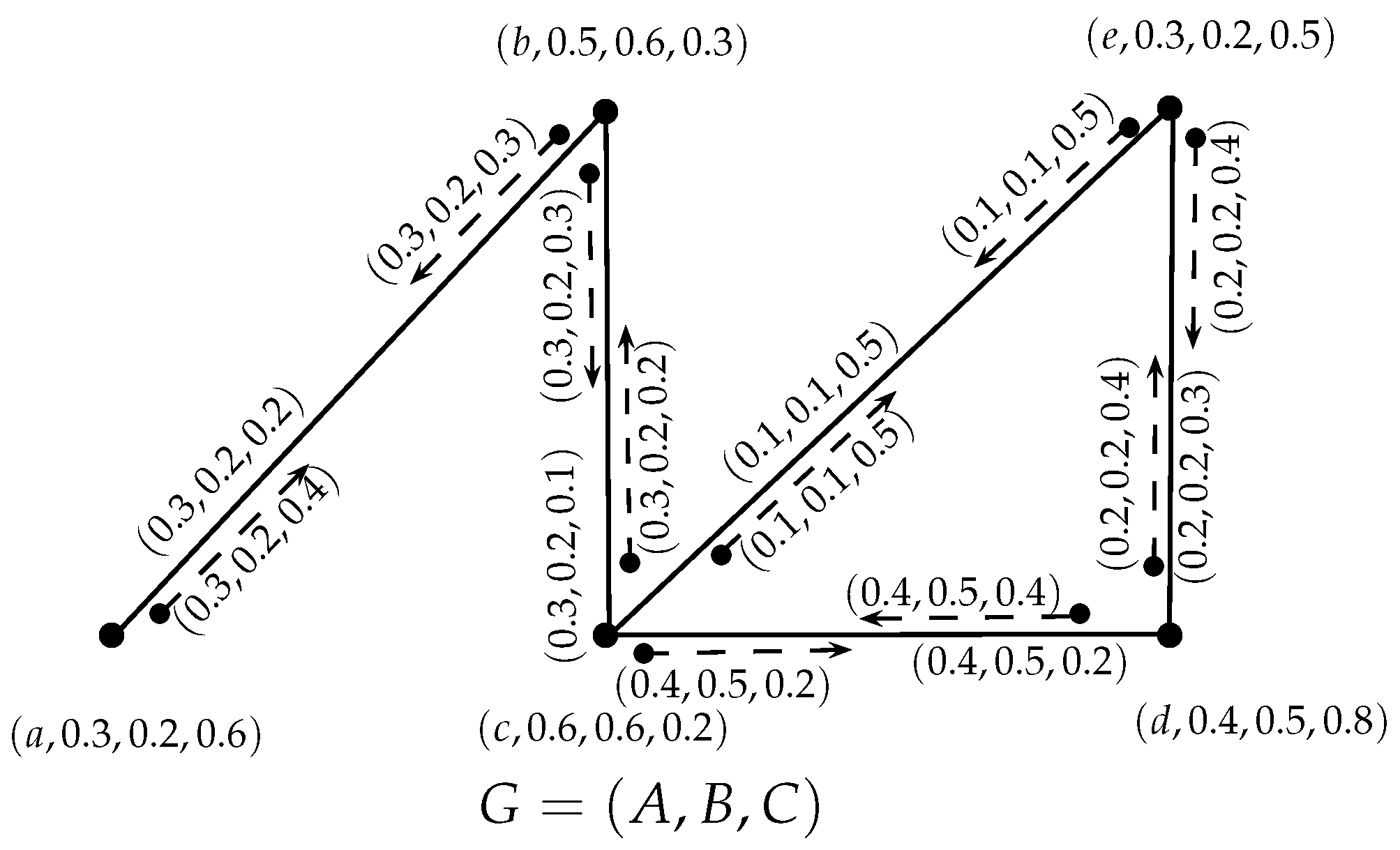
Let $\tilde{G}=$ $(A,B,C)$ be an SVNIG. A pair $(u,uv)$ is called a neutrosophic cutpair if deleting the pair $(u,uv)$ reduces the connectedness between $u,uv\in A^{*}\cup B^{*}$, that is,

$$S^{{}^{\prime }\infty }(u,uv)<S^{\infty }(u,uv),$$

where $S^{{}^{\prime }\infty }(u,uv)$ and $S^{\infty }(u,uv)$ denote the connectedness between u and $uv$ in $G^{{}^{\prime }}=$ $\tilde{G}$ $-\left\{\right(u,uv\left)\right\}$ and $\tilde{G}$, respectively.

A pair $(u,uv)$ is called neutrosophic incidence cutpair if

$$I{S}^{{}^{\prime }\infty }(u,uv)<I{S}^{\infty }(u,uv),\mathit{for}u,uv\in A^{*}\cup B^{*},$$

where $I{S}^{{}^{\prime }\infty }(u,uv)$ and $I{S}^{\infty }(u,uv)$ denote the incidence connectedness between u and $uv$ in $G^{{}^{\prime }}=$ $\tilde{G}$ $-\left\{\right(u,uv\left)\right\}$ and $\tilde{G}$, respectively.

Example 6.

In the SVNIG, $\tilde{G}$, given in Figure 6, $ab$ and $bc$ are bridges, since their removal disconnects the underlying graph, $G^{*}$.

In $\tilde{G}$, $ab$, $bc$, $cd$ and $de$ are neutrosophic bridges, since, for a, e $\in A^{*}$,

$$S^{{}^{\prime }\infty }(a,e)<S^{\infty }(a,e)$$

after the removal of each of the bridges. The edges—$ab$, $bc$, $cd$ and $de$—are neutrosophic incidence bridges in $\tilde{G}$ as well.

b and c are cutvertices. In addition, all the vertices of $\tilde{G}$ are neutrosophic cutvertices, except for a, since the removal of a does not affect the connectedness of $\tilde{G}$. b, c, d and e are neutrosophic incidence cutvertices in $\tilde{G}$.

The pairs $(a,ab)$, $(b,ab)$, $(b,bc)$ and $(c,bc)$ are the cutpairs, neutrosophic cutpairs and also neutrosophic incidence cutpairs in the given graph.

Theorem 1.

Let $\tilde{G}=$ $(A,B,C)$ be a SVNIG. If $uv$ is a neutrosophic bridge, then $uv$ is not a weakest edge in any cycle.

Proof. 

Let $uv$ be a neutrosophic bridge and suppose, on the contrary, that $uv$ is the weakest edge of a cycle. Then, in this cycle, we can find an alternative path, $P_1$, from u to v that does not contain the edge $uv$, and $S\left(P_1\right)$ is greater than or equal to $S\left(P_2\right)$, where $P_2$ is the path involving the edge $uv$. Thus, removal of the edge $uv$ from $\tilde{G}$ does not affect the connectedness between u and v—a contradiction to our assumption. Hence, $uv$ is not the weakest edge in any cycle. ☐

Theorem 2.

If $(u,uv)$ is a neutrosophic incidence cutpair, then $(u,uv)$ is not the weakest pair in any cycle.

Proof. 

Let $(u,uv)$ be a neutrosophic incidence cutpair in $\tilde{G}$. On contrary suppose that $(u,uv)$ is a weakest pair of a cycle. Then we can find an alternative path from u to $uv$ having incidence strength greater than or equal to that of the path involving the pair $(u,uv)$. Thus, removal of the pair $(u,uv)$ does not affect the incidence connectedness between u and $uv$ but this is a contradiction to our assumption that $(u,uv)$ is a neutrosophic incidence cutpair. Hence $(u,uv)$ is not a weakest pair in any cycle. ☐

Theorem 3.

Let $\tilde{G}=$ $(A,B,C)$ be a SVNIG. If $uv$ is a neutrosophic bridge in $\tilde{G}$, then

$$S^{\infty }(u,v)=(s_1^{\infty },s_2^{\infty },s_3^{\infty })=(T_B\left(uv\right),I_B\left(uv\right),F_B\left(uv\right)).$$

Proof. 

Let $\tilde{G}$ be an SVNIG, and uv is a neutrosophic bridge in $\tilde{G}$. On the contrary, suppose that

$$S^{\infty }(u,v)>(T_B\left(uv\right),I_B\left(uv\right),F_B\left(uv\right)).$$

Then, there exists a u-v path, P, with

$$S\left(P\right)>(T_B\left(uv\right),I_B\left(uv\right),F_B\left(uv\right))$$

and

$$(T_B\left(xy\right),I_B\left(xy\right),F_B\left(xy\right))>(T_B\left(uv\right),I_B\left(uv\right),F_B\left(uv\right)),$$

for all edges on path P. Now, P, together with the edge, $uv$, forms a cycle in which $uv$ is the weakest edge, but it is a contradiction to the fact that $uv$ is a neutrosophic bridge. Hence,

$$S^{\infty }(u,v)=(s_1^{\infty },s_2^{\infty },s_3^{\infty })=(T_B\left(uv\right),I_B\left(uv\right),F_B\left(uv\right)).$$

 ☐

Theorem 4.

If $(u,uv)$ is a neutrosophic incidence cutpair in an SVNIG $\tilde{G}$ = $(A,B,C)$, then

$$I{S}^{\infty }(u,uv)=(i{s}_1^{\infty },i{s}_2^{\infty },i{s}_3^{\infty })=(T_C(u,uv),I_C(u,uv),F_C(u,uv)).$$

Proof. 

The proof is on the same line as Theorem 3. ☐

Theorem 5.

Let $\tilde{G}=$ $(A,B,C)$ be an SVNIG and $G^{*}=(A^{*},B^{*},C^{*})$ is a cycle. Then, an edge, $uv$, is a neutrosophic bridge of $\tilde{G}$ if, and only if, it is an edge common to two neutrosophic incidence cutpairs.

Proof. 

Suppose that $uv$ is a neutrosophic bridge of $\tilde{G}$. Then, there exist vertices u and v with the $uv$ edge lying on every path with the greatest incidence strength between u and v. Consequently, there exists only one path, P, (say) between u and v which contains a $uv$ edge and has the greatest incidence strength. Any pair on P will be a neutrosophic incidence cutpair, since the removal of any one of them will disconnect P and reduce the incidence strength.

Conversely, let $uv$ be an edge common to two neutrosophic incidence cutpairs $(u,uv)$ and $(v,uv)$. Thus both $(u,uv)$ and $(v,uv)$ are not the weakest cutpairs of $\tilde{G}$. Now, $G^{*}=(A^{*},B^{*},C^{*})$ being a cycle, there exist only two paths between any two vertices. Also the path $P_1$ from the vertex u to v not containing the pairs $(u,uv)$ and $(v,uv)$ has less incidence strength than the path containing them. Thus, the path with the greatest incidence strength from u to v is

$$P_2:u,(u,uv),uv,(v,uv),v.$$

Also,

$$S^{\infty }(u,v)=S\left(P_2\right)=(T_B\left(uv\right),I_B\left(uv\right),F_B\left(uv\right)).$$

Therefore, $uv$ is a neutrosophic bridge. ☐

Definition 14.

Let $\tilde{G}$ = $(A,B,C)$ be an SVNIG. An edge, $uv$, of $\tilde{G}$ is called a strong edge if

$$S^{{}^{\prime }\infty }(u,v)\le (T_B\left(uv\right),I_B\left(uv\right),F_B\left(uv\right)),$$

where $S^{{}^{\prime }\infty }(u,v)$ represents the connectedness between u and v in $G^{\prime }=$ $\tilde{G}$ $-\left\{uv\right\}$.

In particular, an edge, $uv$, is said to be an α-strong edge if

$$S^{{}^{\prime }\infty }(u,v)<(T_B\left(uv\right),I_B\left(uv\right),F_B\left(uv\right)),$$

and it is called a β-strong edge if

$$S^{{}^{\prime }\infty }(u,v)=(T_B\left(uv\right),I_B\left(uv\right),F_B\left(uv\right)).$$

Definition 15.

A pair $(u,uv)$ in an SVNIG, $\tilde{G}$, is called a strong pair if

$$I{S}^{{}^{\prime }\infty }(u,uv)\le (T_C(u,uv),I_C(u,uv),F_C(u,uv)),$$

where $I{S}^{{}^{\prime }\infty }(u,uv)$ represents the incidence connectedness between u and $uv$ in $G^{\prime }=$ $\tilde{G}$ $-\left\{\right(u,uv\left)\right\}.$

In particular, $(u,uv)$ is called α-strong pair if

$$I{S}^{{}^{\prime }\infty }(u,uv)<(T_C(u,uv),I_C(u,uv),F_C(u,uv)),$$

and it is called β-strong pair if

$$I{S}^{{}^{\prime }\infty }(u,uv)=(T_C(u,uv),I_C(u,uv),F_C(u,uv)).$$

It is not necessary for all edges and pairs to be strong. Edges and pairs exist which are not strong in an SVNIG. Such edges and pairs are given in the following definition.

Definition 16.

Let $\tilde{G}=$ $(A,B,C)$ be an SVNIG. An edge, $uv$, is said to be a δ-edge if

$$(T_B\left(uv\right),I_B\left(uv\right),F_B\left(uv\right))<S^{{}^{\prime }\infty }(u,v).$$

Similarly, a pair $(u,uv)$ in $\tilde{G}$ is called a δ-pair if

$$(T_C(u,uv),I_C(u,uv),F_C(u,uv))<I{S}^{{}^{\prime }\infty }(u,uv).$$

Theorem 6.

In an SVNIG, every neutrosophic incidence cutpair is a strong pair.

Proof. 

Let $\tilde{G}$ = $(A,B,C)$ be an SVNIG. Let $(u,uv)\in C^{*}$ be a neutrosophic incidence cutpair. Then, by  Definition 13, we have

$$I{S}^{{}^{\prime }\infty }(u,uv)<I{S}^{\infty }(u,uv).$$

On the contrary, suppose that $(u,uv)$ is not a strong incidence pair. Then, it follows that

$$I{S}^{{}^{\prime }\infty }(u,uv)>(T_C(u,uv),I_C(u,uv),F_C(u,uv)).$$

Let P be the path from u to $uv$ in $G^{\prime }=$ $\tilde{G}$ $-\left\{\right(u,uv\left)\right\}$ with the greatest incidence strength. Then, P together with $(u,uv)$, forms a cycle in $\tilde{G}$. Now, in this cycle, $(u,uv)$ is the weakest pair, but, based on Theorem 2, it is not possible, since $(u,uv)$ is a neutrosophic incidence cutpair. Hence, our assumption is wrong, and $(u,uv)$ is a strong incidence pair. ☐

Theorem 7.

In an SVNIG $\tilde{G}$ = $(A,B,C).$ The pair $(u,uv)$ is a neutrosophic incidence cutpair if, and only if, it is α-strong.

Proof. 

Let $(u,uv)$ be a neutrosophic incidence cutpair in $\tilde{G}$. Then, according to the Definition 13 of cutpair,

$$I{S}^{\infty }(u,uv)>I{S}^{{}^{\prime }\infty }(u,uv).$$

Then, based on Theorem 4, it follows that

$$(T_C(u,uv),I_C(u,uv),F_C(u,uv))>I{S}^{{}^{\prime }\infty }(u,uv),$$

which is the definition of $\alpha$-strong pair. Hence, $(u,uv)$ is an $\alpha$-strong pair in $\tilde{G}$.

Conversely, let $(u,uv)$ be an $\alpha$-strong pair in $\tilde{G}$. Then, by definition

$$(T_C(u,uv),I_C(u,uv),F_C(u,uv))>I{S}^{{}^{\prime }\infty }(u,uv).$$

It follows that $P:u,(u,uv),uv$ is a unique path from u to $uv$ which has the greatest incidence strength of all paths.Therefore, any other path from u to $uv$ will have a lower incidence strength.

$$I{S}^{\infty }(u,uv)>I{S}^{{}^{\prime }\infty }(u,uv).$$

Hence, $(u,uv)$ is a neutrosophic incidence cutpair. ☐

Definition 17.

Let $\tilde{G}=$ $(A,B,C)$ be an SVNIG.

(i) 

$\tilde{G}$ is called a block if $G^{*}=(A^{*},B^{*},C^{*})$ is block. That is, there are no cutvertices in $G^{*}$.

(ii) 

$\tilde{G}$ is called a neutrosophic block if $\tilde{G}$ has no neutrosophic cutvertices.

(iii) 

$\tilde{G}$ is called a neutrosophic incidence block if it has no neutrosophic incidence cutvertices.

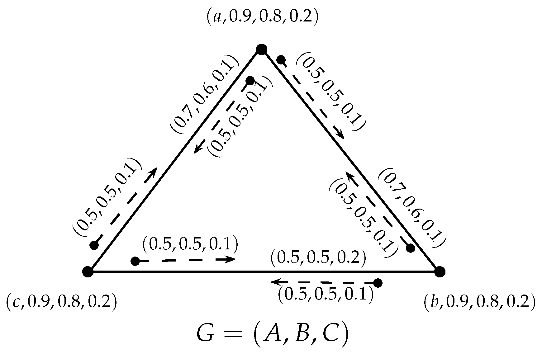
Example 7.

Consider the SVNIG $\tilde{G}=$ $(A,B,C)$ shown in Figure 7 with $A^{*}=\{a,b,c\}$ and $B^{*}=\{ab,bc,ac\}$. $\tilde{G}$ is a block, since the crisp graph, $G^{*}$, has no cutvertex and it is a neutrosophic incidence block. $\tilde{G}$ is not a neutrosophic block, since it has a neutrosophic cutvertex, namely, a.

Theorem 8.

Let $\tilde{G}=$ $(A,B,C)$ be a neutrosophic incidence block. A pair, $(u,uv)$, in $\tilde{G}$, such that

$$(T_C(u,uv),I_C(u,uv),F_C(u,uv))=(max{T}_C(x,xy),max{I}_C(x,xy),min{F}_C(x,xy)),$$

for all $(x,xy)\in C^{*}$, is a strong pair.

Proof. 

Let $\tilde{G}$ be a neutrosophic incidence block. By definition, there are no neutrosophic incidence cutvertices in $\tilde{G}$. Let $(u,uv)$ be a pair in $\tilde{G}$, such that

$$(T_C(u,uv),I_C(u,uv),F_C(u,uv))=(max{T}_C(x,xy),max{I}_C(x,xy),min{F}_C(x,xy)).$$

We will prove that $(u,uv)$ is a strong pair by showing that

$$(T_C(u,uv),I_C(u,uv),F_C(u,uv))\ge I{S}^{{}^{\prime }\infty }(u,uv).$$

The incidence strength of any path, P, from u to $uv$ will be less than or equal to $(T_C(u,uv),I_C(u,uv),F_C(u,uv))$. If $(u,uv)$ is the only pair in $\tilde{G}$ with

$$(T_C(u,uv),I_C(u,uv),F_C(u,uv))=(max{T}_C(x,xy),max{I}_C(x,xy),min{F}_C(x,xy)),$$

then every other path from x to $xy$ in $\tilde{G}$ will have less incidence strength than $(T_C(u,uv),I_C(u,uv),F_C(u,uv))$, and hence,

$$(T_C(u,uv),I_C(u,uv),F_C(u,uv))>I{S}^{{}^{\prime }\infty }(u,uv).$$

Thus, $(u,uv)$ is an $\alpha$-strong pair.

If $(u,uv)$ is not unique, then the maximum possible value for the incidence strength of any path in $G^{{}^{\prime }}=$ $\tilde{G}$ $-\left\{\right(u,uv\left)\right\}$ will be equal to $(T_C(u,uv),I_C(u,uv),F_C(u,uv))$. Therefore, there exists a path from u to $uv$ with an incidence strength equal to $(T_C(u,uv),I_C(u,uv),F_C(u,uv))$, that is

$$(T_C(u,uv),I_C(u,uv),F_C(u,uv))=I{S}^{{}^{\prime }\infty }(u,uv).$$

Then, $(u,uv)$ is $\beta$-strong. ☐

3. Application

According to the Federal Investigation Agency (FIA), Pakistan is among the fourth largest country in terms of its citizens who illegally enter Europe. There is no formally declared policy of the Government of Pakistan for Migration and Pakistani Migrants. Every year, thousands of Pakistanis fleeing poverty, unemployment, law and other problems attempt to illegally enter Europe. A lot of them even die before reaching the destination. These illegal immigrants use land routes featuring Pakistan, Iran, Turkey and Greece to enter Europe. Greece is a gateway to the west, and roughly nine out of ten people illegally entering Europe follow this route. Below, we present a mathematical model of this phenomenon.

Consider SVNIG $\tilde{G}$ = $(A,B,C)$ as shown in Figure 8, a mathematical model of the situation of illegal migration from Pakistan to European, where

$$A=\left\{\right(Pakistan,0.9,0.8,0.7),(Iran,0.8,0.6,0.8),(Turkey,0.9,0.8,0.7),(Greece,0.9,0.8,0.6\left)\right\}$$

is the set of countries under consideration,

$$B=\left\{\right((Pak,Iran),0.7,0.6,0.4),((Iran,Turkey),0.5,0.5,0.5),((Turkey,Greece),0.6,0.8,0.5\left)\right\}$$

represents the flow of people traveling legally from country x to country y and

$$\begin{array}{cc}\hfill C=& \left\{\right((Pak,(Pak,Iran\left)\right),0.5,0.6,0.3),((Iran,(Pak,Iran\left)\right),0.4,0.2,0.8),((Iran,(Iran,Turkey\left)\right),0.5,0.5,0.4),\hfill \\ & \left(\right(Turkey,(Iran,Turkey)),0.3,0.5,0.4),\left(\right(Turkey,(Turkey,Greece)),0.6,0.8,0.2),\hfill \\ & \left(\right(Greece,(Turkey,Greece)),0.2,0.2,0.6)\}\hfill \end{array}$$

represents the flow of people traveling illegally from country x to the country y. It is clear that each pair in this model is a neutrosophic incidence cutpair. So, every government of the countries featuring in this path must make hard and fast rules to control illegal migration as it creates lot of problems for both sending and receiving countries. Policy makers and practitioners need to develop a comprehensive understanding of the phenomenon of illegal migration in order to manage it effectively. We present our proposed method in Algorithm 1.

Algorithm 1 Method of Finding Neutrosophic Incidence Cutpair

Input the vertex set, V. Input the edge set, $E\subseteq V\times V$. Construct the single-valued neutrosophic set, A, on V. Construct the single-valued neutrosophic relation, B, on E. Construct the single-valued neutrosophic set, C, on $V\times E$. Calculate the incidence strength, $IS(u_i,u_j)$, of all possible paths from $u_i$ to $u_j$, such that $$\begin{array}{ccc}\hfill i{s}_1& =& min\{T_C(u_i,u_i{u}_{i+1}):(u_i,u_i{u}_{i+1})\in I\},\hfill \\ \hfill i{s}_2& =& min\{I_C(u_i,u_i{u}_{i+1}):(u_i,u_i{u}_{i+1})\in I\},\hfill \\ \hfill i{s}_3& =& max\{F_C(u_i,u_i{u}_{i+1}):(u_i,u_i{u}_{i+1})\in I\}.\hfill \end{array}$$ Calculate the greatest incidence strength, $I{S}^{\infty }(u_i,u_j)$, of paths from $u_i$ to $u_j$. Remove the pair $(u_i,u_i{u}_{i+1})$ from I. Repeat step 6 and step 7 to calculate the incidence strength, $I{S}^{{}^{\prime }\infty }(u_i,u_j)$ from $u_i$ to $u_j$. Compare the two greatest incidence strengths. If $I{S}^{{}^{\prime }\infty }(u_i,u_j)<I{S}^{\infty }(u_i,u_j)$, then $(u_i,u_i{u}_{i+1})$ is the required neutrosophic incidence cutpair.

4. Conclusions

Graph theory is a useful tool for analyzing and modeling different mathematical structures. However, its failure to determine relationships between vertices (nodes) and edge (arcs) led to the introduction of the fuzzy incidence graph. The single-valued neutrosophic incidence graph is an extension of fuzzy incidence graph, which can be used as a tool for constructing different mathematical models with indeterminate information and interconnected supporting links. In this paper, we discussed different properties of single-valued neutrosophic incidence graphs. We studied the block structure of single-valued neutrosophic incidence graphs. We aim to extend the application of single-valued neutrosophic incidence graphs to human trafficking.